Guest Post by Werner Brozek, Excerpted from Professor Robert Brown from Duke University, Conclusion by Walter Dnes and Edited by Just The Facts:

A while back, I had a post titled: HadCRUT4 is From Venus, GISS is From Mars, which showed wild monthly variations from which one could wonder if GISS and Hadcrut4 were talking about the same planet. In comments, mark stoval, posted a link to this article, Why “GISTEMP LOTI global mean” is wrong and “HadCRUt3 gl” is right“, who’s title speaks for itself and Bob Tisdale has a recent post, Busting (or not) the mid-20th century global-warming hiatus, which could explain the divergence seen in the chart above.
The graphic at the top is the last plot from Professor Brown from his comment I’ve excerpted below, which shows a period of 19 years where the slopes go in opposite directions by a fairly large margin. Is this reasonable? Think about this as you read his comment below. His comment ends with rgb.
rgbatduke
November 10, 2015 at 1:19 pm
“Werner, if you look over the length and breadth of the two on WFT, you will find that over a substantial fraction of the two plots they are offset by less than 0.1 C. For example, for much of the first half of the 20th century, they are almost on top of one another with GISS rarely coming up with a patch 0.1 C or so higher. They almost precisely match in a substantial part of their overlapping reference periods. They only start to substantially split in the 1970 to 1990 range (which contains much of the latter 20th century warming). By the 21st century this split has grown to around 0.2 C, and is remarkably consistent. Let’s examine this in some detail:
We can start with very simple graph that shows the divergence over the last century:
http://www.woodfortrees.org/plot/hadcrut4gl/from:1915/to:2015/trend/plot/gistemp/from:1915/to:2015/trend
The two graphs have widening divergence in the temperatures they obtain. If the two measures were in mutual agreement, one would expect the linear trends to be in good agreement — the anomaly of the anomaly, as it were. They should, after all, be offset by only the difference in mean temperatures in their reference periods, which should be a constant offset if they are both measuring the correct anomalies from the same mean temperatures.
Obviously, they do not. There is a growing rift between the two and, as I noted, they are split by more than the 95% confidence that HadCRUT4, at least, claims even relative to an imagined split in means over their reference periods. There are, very likely, nonlinear terms in the models used to compute the anomalies that are growing and will continue to systematically diverge, simply because they very likely have different algorithms for infilling and kriging and so on, in spite of them very probably having substantial overlap in their input data.
In contrast, BEST and GISS do indeed have similar linear trends in the way expected, with a nearly constant offset. One presumes that this means that they use very similar methods to compute their anomalies (again, from data sets that very likely overlap substantially as well). The two of them look like they want to vote HadCRUT4 off of the island, 2 to 1:
http://www.woodfortrees.org/plot/hadcrut4gl/from:1915/to:2005/trend/plot/gistemp/from:1915/to:2005/trend/plot/best/from:1915/to:2005/trend
Until, of course, one adds the trends of UAH and RSS:
http://www.woodfortrees.org/plot/hadcrut4gl/from:1979/to:2015/trend/plot/gistemp/from:1979/to:2015/trend/plot/best/from:1979/to:2005/trend/plot/rss/from:1979/to:2015/trend/plot/uah/from:1979/to:2015/trend
All of a sudden consistency emerges, with some surprises. GISS, HadCRUT4 and UAH suddenly show almost exactly the same linear trend across the satellite era, with a constant offset of around 0.5 C. RSS is substantially lower. BEST cannot honestly be compared, as it only runs to 2005ish.
One is then very, very tempted to make anomalies out of our anomalies, and project them backwards in time to see how well they agree on hind casts of past data. Let’s use the reference period show and subtract around 0.5 C from GISS and 0.3 C from HadCRUT4 to try to get them to line up with UAH in 2015 (why not, good as any):
http://www.woodfortrees.org/plot/hadcrut4gl/from:1979/to:2015/offset:-0.32/trend/plot/gistemp/from:1979/to:2015/offset:-0.465/trend/plot/uah/from:1979/to:2015/trend
We check to see if these offsets do make the anomalies match over the last 36 most accurate years (within reason):
http://www.woodfortrees.org/plot/hadcrut4gl/from:1979/to:2015/offset:-0.32/plot/gistemp/from:1979/to:2015/offset:-0.465/plot/uah/from:1979/to:2015
and see that they do. NOW we can compare the anomalies as they project into the indefinite past. Obviously UAH does have a slightly slower linear trend over this “re-reference period” and it doesn’t GO any further back, so we’ll drop it, and go back to 1880 to see how the two remaining anomalies on a common base look:
http://www.woodfortrees.org/plot/hadcrut4gl/from:1880/to:2015/offset:-0.32/plot/gistemp/from:1880/to:2015/offset:-0.465
We now might be surprised to note that HadCRUT4 is well above GISS LOTI across most of its range. Back in the 19th century splits aren’t very important because they both have error bars back there that can forgive any difference, but there is a substantial difference across the entire stretch from 1920 to 1960:
http://www.woodfortrees.org/plot/hadcrut4gl/from:1920/to:1960/offset:-0.32/plot/gistemp/from:1920/to:1960/offset:-0.465/plot/hadcrut4gl/from:1920/to:1960/offset:-0.32/trend/plot/gistemp/from:1920/to:1960/offset:-0.465/trend
This reveals a robust and asymmetric split between HadCRUT4 and GISS LOTI that cannot be written off to any difference in offsets, as I renormalized the offsets to match them across what has to be presumed to be the most precise and accurately known part of their mutual ranges, a stretch of 36 years where in fact their linear trends are almost precisely the same so that the two anomalies differ only BY an offset of 0.145 C with more or less random deviations relative to one another.
We find that except for a short patch right in the middle of World War II, HadCRUT4 is consistently 0.1 to 0.2 C higher than GISStemp. This split cannot be repaired — if one matches it up across the interval from 1920 to 1960 (pushing GISStemp roughly 0.145 HIGHER than HadCRUT4 in the middle of WW II) then one splits it well outside of the 95% confidence interval in the present.
Unfortunately, while it is quite all right to have an occasional point higher or lower between them — as long as the “occasions” are randomly and reasonably symmetrically split — this is not an occasional point. It is a clearly resolved, asymmetric offset in matching linear trends. To make life even more interesting, the linear trends do (again) have a more or less matching slope, across the range 1920 to 1960 just like they do across 1979 through 2015 but with completely different offsets. The entire offset difference was accumulated from 1960 to 1979.
Just for grins, one last plot:
http://www.woodfortrees.org/plot/hadcrut4gl/from:1880/to:1920/offset:-0.365/plot/gistemp/from:1880/to:1920/offset:-0.465/plot/hadcrut4gl/from:1880/to:1920/offset:-0.365/trend/plot/gistemp/from:1880/to:1920/offset:-0.465/trend
Now we have a second, extremely interesting problem. Note that the offset between the linear trends here has shrunk to around half of what it was across the bulk of the early 20th century with HadCRUT4 still warmer, but now only warmer by maybe 0.045 C. This is in a region where the acknowledged 95% confidence range is order of 0.2 to 0.3. When I subtract appropriate offsets to make the linear trends almost precisely match in the middle, we get excellent agreement between the two anomalies.
Too excellent. By far. All of the data is within the mutual 95% confidence interval! This is, believe it or not, a really, really bad thing if one is testing a null hypothesis such as “the statistics we are publishing with our data have some meaning”.
We now have a bit of a paradox. Sure, the two data sets that these anomalies are built from very likely have substantial overlap, so the two anomalies themselves cannot properly be viewed as random samples drawn from a box filled with independent and identically distributed but correctly computed anomalies. But their super-agreement across the range from 1880 to 1920 and 1920 to 1960 (with a different offset) and across the range from 1979 to 2015 (but with yet another offset) means serious trouble for the underlying methods. This is absolutely conclusive evidence, in my opinion, that “According to HadCRUT4, it is well over 99% certain GISStemp is an incorrect computation of the anomaly” and vice versa. Furthermore, the differences between the two can not be explained by the fact that they draw on partially independent data sources — if this were the case, the strong coincidences between the two across piecewise blocking of the data are too strong — obviously the independent data is not sufficient to generate a symmetric and believable distribution of mutual excursions with errors that are anywhere near as large as they have to be, given that both HadCRUT4 and GISStemp if anything underestimate probable errors in the 19th century.
Where is the problem? Well, as I noted, a lot of it happens right here:
http://www.woodfortrees.org/plot/hadcrut4gl/from:1960/to:1979/offset:-0.32/plot/gistemp/from:1960/to:1979/offset:-0.465/plot/hadcrut4gl/from:1960/to:1979/offset:-0.32/trend/plot/gistemp/from:1960/to:1979/offset:-0.465/trend
The two anomalies match up almost perfectly from the right hand edge to the present. They do not match up well from 1920 to 1960, except for a brief stretch of four years or so in early World War II, but for most of this interval they maintain a fairly constant, and identical, slope to their (offset) linear trend! They match up better (too well!) — with again a very similar linear trend but yet another offset across the range from 1880 to 1920. But across the range from 1960 to 1979, Ouch! That’s gotta hurt. Across 20 years, HadCRUT4 cools Earth by around 0.08 C, while GISS warms it by around around 0.07C.
So what’s going on? This is a stretch in the modern era, after all. Thermometers are at this point pretty accurate. World History seems to agree with HadCRUT4, since in the early 70’s there was all sorts of sound and fury about possible ice ages and global cooling, not global warming. One would expect both anomalies to be drawing on very similar data sets with similar precision and with similar global coverage. Yet in this stretch of the modern era with modern instrumentation and (one has to believe) very similar coverage, the two major anomalies don’t even agree in the sign of the linear trend slope and more or less symmetrically split as one goes back to 1960, a split that actually goes all the way back to 1943, then splits again all the way back to 1920, then slowly “heals” as one goes back to 1880.
As I said, there is simply no chance that HadCRUT4 and GISS are both correct outside of the satellite era. Within the satellite era their agreement is very good, but they split badly over the 20 years preceding it in spite of the data overlap and quality of instrumentation. This split persists over pretty much the rest of the mutual range of the two anomalies except for a very short period of agreement in mid-WWII, where one might have been forgiven for a maximum disagreement given the chaotic nature of the world at war. One must conclude, based on either one, that it is 99% certain that the other one is incorrect.
Or, of course, that they are both incorrect. Further, one has to wonder about the nature of the errors that result in a split that is so clearly resolved once one puts them on an equal footing across the stretch where one can best believe that they are accurate. Clearly it is an error that is a smooth function of time, not an error that is in any sense due to accuracy of coverage of the (obviously strongly overlapping) data.
This result just makes me itch to get my hands on the data sets and code involved. For example, suppose that one feeds the same data into the two algorithms. What does one get then? Suppose one keeps only the set of sites that are present in 1880 when the two have mutually overlapping application (or better, from 1850 to the present) and runs the algorithm on them. How much do the results split from a) each other; and b) the result obtained from using all of the available sites in the present? One would expect the latter, in particular, to be a much better estimator of the probable method error in the remote past — if one uses only those sites to determine the current anomaly and it differs by (say) 0.5 C from what one gets using all sites, that would be a very interesting thing in and of itself.
Finally, there is the ongoing problem with using anomalies in the first place rather than computing global average temperatures. Somewhere in there, one has to perform a subtraction. The number you subtract is in some sense arbitrary, but any particular number you subtract comes with an error estimate of its own. And here is the rub:
The place where the two global anomalies develop their irreducible split is square inside the mutually overlapping part of their reference periods!
That is, the one place they most need to be in agreement, at least in the sense that they reproduce the same linear trends, that is, the same anomalies is the very place where they most greatly differ. Indeed, their agreement is suspiciously good — as far as linear trend is concerned – everywhere else, in particular in the most recent present where one has to presume that the anomaly is most accurately being computed and the most remote past where one expects to get very different linear trends but instead get almost identical ones!
I doubt that anybody is still reading this thread to see this — but they should.
rgb
P.S. from Werner Brozek:
On Nick Stokes Temperature Trend Viewer note the HUGE difference in the lower number for the 95% (Cl) confidence limits between Hadcrut4 and GISS from March 2005 to April 2016:
For GISS:
Temperature Anomaly trend
Mar 2005 to Apr 2016
Rate: 2.199°C/Century;
CI from 0.433 to 3.965;
For Hadcrut4:
Temperature Anomaly trend
Mar 2005 to Apr 2016
Rate: 1.914°C/Century;
CI from -0.023 to 3.850;
In the sections below, we will present you with the latest facts. The information will be presented in two sections and an appendix. The first section will show for how long there has been no statistically significant warming on several data sets. The second section will show how 2016 so far compares with 2015 and the warmest years and months on record so far. For three of the data sets, 2015 also happens to be the warmest year. The appendix will illustrate sections 1 and 2 in a different way. Graphs and a table will be used to illustrate the data. The two satellite data sets go to May and the others go to April.
Section 1
For this analysis, data was retrieved from Nick Stokes’ Trendviewer available on his website. This analysis indicates for how long there has not been statistically significant warming according to Nick’s criteria. Data go to their latest update for each set. In every case, note that the lower error bar is negative so a slope of 0 cannot be ruled out from the month indicated.
On several different data sets, there has been no statistically significant warming for between 0 and 23 years according to Nick’s criteria. Cl stands for the confidence limits at the 95% level.
The details for several sets are below.
For UAH6.0: Since May 1993: Cl from -0.023 to 1.807
This is 23 years and 1 month.
For RSS: Since October 1993: Cl from -0.010 to 1.751
This is 22 years and 8 months.
For Hadcrut4.4: Since March 2005: Cl from -0.023 to 3.850
This is 11 years and 2 months.
For Hadsst3: Since July 1996: Cl from -0.014 to 2.152
This is 19 years and 10 months.
For GISS: The warming is significant for all periods above a year.
Section 2
This section shows data about 2016 and other information in the form of a table. The table shows the five data sources along the top and other places so they should be visible at all times. The sources are UAH, RSS, Hadcrut4, Hadsst3, and GISS.
Down the column, are the following:
1. 15ra: This is the final ranking for 2015 on each data set.
2. 15a: Here I give the average anomaly for 2015.
3. year: This indicates the warmest year on record so far for that particular data set. Note that the satellite data sets have 1998 as the warmest year and the others have 2015 as the warmest year.
4. ano: This is the average of the monthly anomalies of the warmest year just above.
5. mon: This is the month where that particular data set showed the highest anomaly prior to 2016. The months are identified by the first three letters of the month and the last two numbers of the year.
6. ano: This is the anomaly of the month just above.
7. sig: This the first month for which warming is not statistically significant according to Nick’s criteria. The first three letters of the month are followed by the last two numbers of the year.
8. sy/m: This is the years and months for row 7.
9. Jan: This is the January 2016 anomaly for that particular data set.
10. Feb: This is the February 2016 anomaly for that particular data set, etc.
14. ave: This is the average anomaly of all months to date taken by adding all numbers and dividing by the number of months.
15. rnk: This is the rank that each particular data set would have for 2016 without regards to error bars and assuming no changes. Think of it as an update 20 minutes into a game.
| Source | UAH | RSS | Had4 | Sst3 | GISS |
|---|---|---|---|---|---|
| 1.15ra | 3rd | 3rd | 1st | 1st | 1st |
| 2.15a | 0.261 | 0.358 | 0.746 | 0.592 | 0.87 |
| 3.year | 1998 | 1998 | 2015 | 2015 | 2015 |
| 4.ano | 0.484 | 0.550 | 0.746 | 0.592 | 0.87 |
| 5.mon | Apr98 | Apr98 | Dec15 | Sep15 | Dec15 |
| 6.ano | 0.743 | 0.857 | 1.010 | 0.725 | 1.10 |
| 7.sig | May93 | Oct93 | Mar05 | Jul96 | |
| 8.sy/m | 23/1 | 22/8 | 11/2 | 19/10 | |
| 9.Jan | 0.540 | 0.665 | 0.908 | 0.732 | 1.11 |
| 10.Feb | 0.832 | 0.978 | 1.061 | 0.611 | 1.33 |
| 11.Mar | 0.734 | 0.842 | 1.065 | 0.690 | 1.29 |
| 12.Apr | 0.715 | 0.757 | 0.926 | 0.654 | 1.11 |
| 13.May | 0.545 | 0.525 | |||
| 14.ave | 0.673 | 0.753 | 0.990 | 0.671 | 1.21 |
| 15.rnk | 1st | 1st | 1st | 1st | 1st |
If you wish to verify all of the latest anomalies, go to the following:
For UAH, version 6.0beta5 was used. Note that WFT uses version 5.6. So to verify the length of the pause on version 6.0, you need to use Nick’s program.
http://vortex.nsstc.uah.edu/data/msu/v6.0beta/tlt/tltglhmam_6.0beta5.txt
For RSS, see: ftp://ftp.ssmi.com/msu/monthly_time_series/rss_monthly_msu_amsu_channel_tlt_anomalies_land_and_ocean_v03_3.txt
For Hadcrut4, see: http://www.metoffice.gov.uk/hadobs/hadcrut4/data/current/time_series/HadCRUT.4.4.0.0.monthly_ns_avg.txt
For Hadsst3, see: https://crudata.uea.ac.uk/cru/data/temperature/HadSST3-gl.dat
For GISS, see:
http://data.giss.nasa.gov/gistemp/tabledata_v3/GLB.Ts+dSST.txt
To see all points since January 2015 in the form of a graph, see the WFT graph below. Note that UAH version 5.6 is shown. WFT does not show version 6.0 yet. Also note that Hadcrut4.3 is shown and not Hadcrut4.4, which is why many months are missing for Hadcrut.

As you can see, all lines have been offset so they all start at the same place in January 2015. This makes it easy to compare January 2015 with the latest anomaly.
Appendix
In this part, we are summarizing data for each set separately.
UAH6.0beta5
For UAH: There is no statistically significant warming since May 1993: Cl from -0.023 to 1.807. (This is using version 6.0 according to Nick’s program.)
The UAH average anomaly so far for 2016 is 0.673. This would set a record if it stayed this way. 1998 was the warmest at 0.484. The highest ever monthly anomaly was in April of 1998 when it reached 0.743 prior to 2016. The average anomaly in 2015 was 0.261 and it was ranked 3rd.
RSS
For RSS: There is no statistically significant warming since October 1993: Cl from -0.010 to 1.751.
The RSS average anomaly so far for 2016 is 0.753. This would set a record if it stayed this way. 1998 was the warmest at 0.550. The highest ever monthly anomaly was in April of 1998 when it reached 0.857 prior to 2016. The average anomaly in 2015 was 0.358 and it was ranked 3rd.
Hadcrut4.4
For Hadcrut4: There is no statistically significant warming since March 2005: Cl from -0.023 to 3.850.
The Hadcrut4 average anomaly so far is 0.990. This would set a record if it stayed this way. The highest ever monthly anomaly was in December of 2015 when it reached 1.010 prior to 2016. The average anomaly in 2015 was 0.746 and this set a new record.
Hadsst3
For Hadsst3: There is no statistically significant warming since July 1996: Cl from -0.014 to 2.152.
The Hadsst3 average anomaly so far for 2016 is 0.671. This would set a record if it stayed this way. The highest ever monthly anomaly was in September of 2015 when it reached 0.725 prior to 2016. The average anomaly in 2015 was 0.592 and this set a new record.
GISS
For GISS: The warming is significant for all periods above a year.
The GISS average anomaly so far for 2016 is 1.21. This would set a record if it stayed this way. The highest ever monthly anomaly was in December of 2015 when it reached 1.10 prior to 2016. The average anomaly in 2015 was 0.87 and it set a new record.
Conclusion
If GISS and Hadcrut4 cannot both be correct, could the following be a factor:
* “Hansen and Imhoff used satellite images of nighttime lights to identify stations where urbanization was most likely to contaminate the weather records.” GISS
* “Using the photos, a citizen science project called Cities at Night has discovered that most light-emitting diodes — which are touted for their energy-saving properties — actually make light pollution worse. The changes in some cities are so intense that space station crew members can tell the difference from orbit.” Tech Insider
Question… is the GISS “nightlighting correction” valid any more? And what does that do to their “data”?
Data Updates
GISS for May came in at 0.93. While this is the warmest May on record, it is the first time that the anomaly fell below 1.00 since October 2015. As for June, present indications are that it will drop by at least 0.15 from 0.93. All months since October 2015 have been record warm months so far for GISS. Hadsst3 for May came in at 0.595. All months since April 2015 have been monthly records for Hadsst3.
Discover more from Watts Up With That?
Subscribe to get the latest posts sent to your email.
Steven Mosher says:
“stop using WFT”
The article uses WoodForTrees (WFT), and the authors posted at least eleven charts derived from the WFT databases. The authors also use Nick Stokes’ Trendviewer, and other data.
Why should we stop using the WoodForTrees databases? Have my donations to WFT been wasted? Please explain why. Do you think WFT manipulates/adjusts the databases it uses, like GISS, BEST, NOAA, UAH, RSS, and others?
Correct me if I’m wrong, but as I understand it WFT simply collates data and automatically produces charts based on whatever data, time frames, trends, and other inputs the user desires. It is a very useful tool. That’s why it is used by all sides in the ‘climate change’ debate.
But now you’re telling us to stop using WFT. Why? You need to explain why you don’t want readers using that resource.
If you have a credible explanation and a better alternative, I for one am easy to convince. I think most readers here can also be convinced — if you can give us convincing reasons.
But just saying “stop using WFT” seems to be due to the fact that WFT products (charts) are different than your BEST charts. Otherwise, what difference would it make?
I’m a reasonable guy, Steven, like most folks here. So give us good reasons why we should stop using WoodForTrees. Then tell us what you think would be the ‘BEST’ charts to use. ☺
Try to be convincing, Steven. Because those hit ‘n’ run comments don’t sway most readers. Neither does telling us what databases, charts, and services we should “stop using”.
WFT is great for those data sets where it is up to date. For the 5 that I report on, that only applies to RSS and GISS. Steven Mosher was responding to my comment just above it here:
https://wattsupwiththat.com/2016/06/16/can-both-giss-and-hadcrut4-be-correct-now-includes-april-and-may-data/comment-page-1/#comment-2238588
In addition to what I said there, WFT is terrible for BEST since there was a huge error in 2010 that has long since been corrected but WFT has not made that correction 6 years later.
As well, it does not do NOAA.
If you can use any influence you have to get WFT to update things, it would be greatly appreciated by many!
“Correct me if I’m wrong, but as I understand it WFT simply collates data and automatically produces charts based on whatever data, time frames, trends, and other inputs the user desires. It is a very useful tool. That’s why it is used by all sides in the ‘climate change’ debate.
But now you’re telling us to stop using WFT. Why? You need to explain why you don’t want readers using that resource.”
As I explained. WTF is a secondary source. Go read the site yourself and see what the author tells you about using the routines.
As a secondary source you dont know
A) if the data has been copied correctly
B) if the algorithms are in fact accurate.
You also know just by looking that one of its sources is bungled.
and further since it allows you to compare data without MASKING for spatial coverage you can be pretty
sure that the comparisons are…… WRONG
SO, if you are a real skeptic you’ll always want to check that you got the right data. if you are trusting WFT
you are not checking now are you?
yes I know its a easy resource to “create’ science on the fly.. but only a fake sceptic would put any trust in the charts. I used it before and finally decided that it was just better to do things right.
dbstealey on June 17, 2016 at 10:57 am
Why should we stop using the WoodForTrees databases? Have my donations to WFT been wasted? Please explain why. Do you think WFT manipulates/adjusts the databases it uses, like GISS, BEST, NOAA, UAH, RSS, and others?
1a. No, db, your donations (not to to WFTbut to Woodland Trust) weren’t wasted, nor did mine. Simply because Paul’s Charity Tip Jar never was intended to be a source of revenue helping him in continuing his pretty good work.
1b. No, db, Paul Clark never manipulated anybody. Much rather was his work unluckily misused by people who clearly intended to manipulate.
2. But the slight difference in output between e.g.
http://www.woodfortrees.org/plot/hadcrut3gl/from:1880
and
http://www.woodfortrees.org/plot/hadcrut4gl/from:1880
might be a helpful hint for you to think about what happens there since longer time…
Even HadCRUT4 was halted at WFT in 2014, but it seems that nobody notices such ‘details’.
And what many people still ignore: Paul Clark’s UAH record still is based on V5.6.
It’s simple to detect: the trend visible from 1979 on the charts is about 0.15 °C / dec.
Ignored as well, especially in this guest post: the BEST record (I mean of course Berkeley Earth’s) is at WFT land only since beginning !!!
Thus comparing this record with GISS and HadCRUT by using WFT is bare ignorance.
3. There are many other reasons not to use WFT when one is not aware of basics concerning temperature anomaly series.
One of the most important ones, discarded even in this post at many places, is the fact that you can’t barely compare two temperature series when they don’t share a common baseline.
Even Bob Tisdale has repeatedly told about the necessity to normalize chart output to have all components on the same baseline.
Thus when I read: We can start with very simple graph that shows the divergence over the last century:
http://www.woodfortrees.org/plot/hadcrut4gl/from:1915/to:2015/trend/plot/gistemp/from:1915/to:2015/trend
I can only answer that this is simply inaccurate: while HadCRUT has an anomaly baseline at 1961:1990, GISSTEMP has it at 1951:2000.
That’s the reason why e.g. Japan’s Meteorology Agency, while internally still handling anomalies based on 1971-2000, nevertheless publishes all data baselined w.r.t. UAH (1981-2010).
And so should do at WUWT every person publishing information on temperature records.
Not because UAH’s baseline would be by definition the best choice, but simply because this 30 year period is the only one meaningfully encompassing the entire satellite era. RSS’ period (1979-1998) is a bit too small.
Thus everybody is kindly invited to publish WFT charts (if s/he can’t do else) with accurate offset information making comparisons meaningful, by normalizing all data e.g. wrt UAH.
GISSTEMP and Berkeley Earth: -0.428
HadCRUT: -0.294
RSS: -0.097
4. And everyone also is invited to produce running mean based charts instead of often useless trends:
http://www.woodfortrees.org/plot/uah/from:1979/mean:37/plot/rss/from:1979/mean:37/offset:-0.097/plot/gistemp/from:1979/mean:37/offset:-0.428/plot/hadcrut4gl/from:1979/mean:37/offset:-0.294
simply because it tells you much more than
http://www.woodfortrees.org/plot/uah/from:1979/trend/plot/rss/from:1979/trend/offset:-0.097/plot/gistemp/from:1979/trend/offset:-0.428/plot/hadcrut4gl/from:1979/trend/offset:-0.294
5. But… the better choices for good information are in my (!) opinion
https://moyhu.blogspot.de/p/temperature-trend-viewer.html
http://www.ysbl.york.ac.uk/~cowtan/applets/trend/trend.html
(though Kevin Cowtan unfortunately didn’t manage to introduce UAH6.0beta5 yet: he awaits peer review results still to be published by Christy/Spencer).
… GISSTEMP has it at 1951:2000.
Wow, apologies: should be read 1951:1980!
It was a clash with NOAA’s good old baseline (1901:2000).
Keep in mind that a change in baseline will not change a negative slope into a positive slope. See the graph at the very start.
Steven Mosher,
Your statement (“stop using WFT”), applies to everyone who uses WFT charts, correct?
But as Werner wrote, the example he posted had already been resolved:
As for this analysis, we had to use the old 4.3, but I checked my top graph against 4.4 using Nick’s graphs and there was not much difference.
If and when the authors of these articles, like Werner Brozek, Prof Robert Brown, Walter Dnes, and other respected scientists who comment here also tell us to “stop using WFT”, then I’ll stop, too.
Their expert opinion sets a reasonable bar, no? That would be convincing to me. But simply finding that a data set needs updating or that a mistake was made and since corrected is no reason to give up the excellent resource that Paul Clark maintains. And as he says, he takes no sides in the climate debate.
But someone who doesn’t want folks to use WFT can’t just say something is wrong, and instruct everyone to stop using that “secondary” data source. They have to post their own chart and show where and why the other one is wrong.
It also needs to show a significant difference. Because as Werner wrote above, “there was not much difference” between the two. And then there are spliced charts like this Moberg nonsense that are so clearly alarmist propaganda that it’s just nitpicking to criticize WFT for using data that isn’t the most up to date version.
And unfortunately, Steven Mosher doesn’t understand scientific skepticism. Sorry, but that’s apparent from his constant taunts. A skeptic’s position is simply this: show us! Produce convincing, empirical, testable evidence to support your hypothesis (such as Mr. Mosher’s statement that CO2 is the primary cause of global warming).
But there’s no observed cause and effect, or other evidence showing that human CO2 emissions cause any measurable global warming. I’ve said many times here that I think a rise in CO2 has a small warming effect. But AGW is simply too small to measure with current instruments. So while AGW may well exist, unless it makes a discernable difference (the Null Hypothesis), it’s just as much a non-problem as if it doesn’t exist.
A multitude of measurements have shown that current global temperatures have not come close to reaching past temperatures, even during the earlier Holocene, when global temperatures varied far more and rose higher than during the past century.
Compared with past temperature records, the fluctuation of only ≈0.7ºC over a century is just a wiggle. If CO2 had the claimed effect, the past century’s one-third rise in CO2 (from below 300 ppm to over 400 ppm) would have caused an unusually large rise in global warming by now, and that global warming would be accelerating. But instead of rising, global warming stopped for many years!
I often think of what Popper and Feynman would have said about that contrary evidence. Even more to the point, I think Prof Langmuir would apply his “Pathological Science” test questions to AGW, which has no more evidence to support it than ‘N-Rays’, or the ‘Allison Effect’, or the ‘Davis-Barnes Effect’, or other examples of scientists believing in things that seem to appear only at the very edge of perception — and which disappear entirely when direct measurements are attempted.
The basic debate has always been over the hypothesis that the rise in human-emitted CO2 will cause runaway global warming. But after many decades that hypothesis has been falsified by empirical observations, and as a result ‘runaway global warming’ has morphed into the vague term ‘climate change’. But the claimed cause of the ‘carbon’ scare remains the same: human CO2 emissions. That, despite the fact that human activity accounts for only one CO2 molecule out of every 34 emitted; the other 33 are natural.
A skeptic should also compare past CO2 and temperature changes with current observations. If the cause and effect is not apparent, it is the skeptics’ job to question the basic premise: the hypothesis that CO2 is the control knob of global temperatures.
But again, where is the evidence? Where are the corroborating observations? They are nowhere to be found. The CO2=CAGW scare is a false alarm because the hypothesis that CO2 is the primary driver of global temperatures has been falsified by decades of real world observations.
So why are we still arguing about a falsified hypothesis? I suspect that the $1 billion+ in annual grants to ‘study climate change’ is a much bigger reason than its proponents will admit.
Werner Brozek June 17, 2016 at 4:53 pm
To be honest: that’s a point I don’t need to be reminded of, I guess.
But what I mean I had underlined more than once (but probably still not enough) is that not using correct baselines when presenting concurrent time series leads to confusion and even to manipulation, be it intended or not.
When having a look at
http://fs5.directupload.net/images/160618/ngwgzhl7.jpg
everybody lacking neccessary knowledge will cry: “Woaaahhh! Oh my…! Look at these manipulators, these GISSes, NOAAs and other
BESTsWORSEs! They make our world much warmer than it is!”How should they know that it in fact looks like this?
http://fs5.directupload.net/images/160618/znpoexoe.jpg
But I’d well agree with you if you answered that there are many more subtle ways to manipulate!
The best example this year was a comparison between radiosondes and satellites, made in order to show how good they fit together, by not only restricting the comparison to the USA, but moreover silently selecting, among the 127 US radiosondes within the IGRA dataset, those 31 promising the very best fit…
Perfect job, Prof. JC!
Hi Bindidon,
Thanks for your charts, which clearly show the planet’s recovery from the LIA. It’s all good!
Adding charts that cover a longer time frame gives readers a more complete picture. More data is always helpful for reaching a conclusion. So in addition to your charts, I’ve posted some that cover a longer time frame, show longer trend lines, or provide other data such as CO2 comparisons, etc.
First, notice that global warming is rising on a steady slope with no acceleration.
Conclusion: CO2 cannot be the major cause of global warming.
In fact, CO2 might not be a cause at all; we just don’t know yet.
But we DO know that like NOAA, NASA also ‘adjusts’ the temperature record — and those manipulations always end up showing more global warming:
http://icecap.us/images/uploads/NASACHANGES.jpg
NOAA does the same thing:
NOAA has changed the past anomaly record at least 96 times in just the past 8 years.
James Hansen began the GISS ‘adjustments’ showing fake warming more than 35 years ago:
http://realclimatescience.com/wp-content/uploads/2016/05/2016-05-09050642.gif
And NASA/GISS continues to alter the past temperature record by erasing and replacing prior records:
http://realclimatescience.com/wp-content/uploads/2016/06/2016-06-10070042-1.png
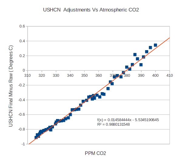
We would expect USHCN, which is another gov’t agency, to follow suit. This shows that as CO2 rises, so do USHCN’s temperature ‘adjustments’:
And despite your charts, it seems that GISS and NOAA are still diverging from satellite data:
http://oi62.tinypic.com/2yjq3pf.jpg
Claiming that there is no manipulation sounds like Bill Cosby protesting that all the women are lying. That might be believable, if it was just one or two women. But when it becomes dozens, his believability is shot.
Like Bill’s accusers, I can post dozens more charts, from many different sources, all showing the same ‘adjustments’ that either adjust the past cooler, or the present hotter, or both. Just say the word, and I’ll post them.
And finally, your WFT charts are appreciated. Almost everyone uses them.
WUW Goddard? He’s overlaid NCAR Northern Hemisphere land-only temps with what? Probably the global record with SSTs.
I made a plot with current GISS NH land-only temp plot with 5 year averages like the NCAR ’74 plot, from 1900-1974, 5-year averages centred on 1902, 1907, etc. NCAR ’74 appear to have centred their 5 yr averages on 1900, 1905 etc, so there will be some differences, but the basic profile is similar…
http://i1006.photobucket.com/albums/af185/barryschwarz/giss%205%20year%20average%20land%20only%20stations%20nh_zpsaejz0c1v.png?t=1466223028
The cooling through mid-century is still apparent. I don’t know what Goddard has done, but he hasn’t done it right, as usual.
(Straight from current GISS data base – divide by 100 to get degrees C anomalies according to their baseline)
One major difference is that there is now 10x more data for weather stations than they had in 1974. Is anyone contending that 10x less data should produce a superior result? That seems to be the implication in many posts here.
And finally, your WFT charts are appreciated.
Cool, then you’ll appreciate this plot of UAH data from 1998 to present.
http://www.woodfortrees.org/graph/uah/from:1998/plot/uah/from:1998/trend
Linear trend is currently 0.12C/decade from 1998.
You’re not going to change your mind about WFT now, are you?
UAH has revised its data set more than a dozen times, sometimes with very significant changes. For example, the 1998 adjustment for orbital decay increased the trend by 0.1C.
UAH are not criticised by skeptics for making adjustments. They are congratulated for it. Skeptics think:
GHCN adjustments = fraud
UAH adjustments = scientific integrity
Skeptics aren’t against adjustments per se. It’s just a buzzword to argue temps are cooler than we think. And to smear researchers. Spencer and Christy seem to be immune. Animal Farm comes to mind. Some pigs are more equal than others.
Some commenters, losing our time by always suspecting that GISS or NOAA temperaure series would be subject of huge adjustments, should be honest enough to download UAH’s data in the revisions 5.6 and 6.0beta5, and to compare them using e.g. Excel.
It is quite easy to construct an Excel table showing, for all 27 zones provided by UAH, the differences between the two revisions, and to plot the result.
Maybe they then begin to understand how small the different surface temperature adjustments applied to GISS, NOAA and HadCRUT were in comparison with that made in april 2015 for UAH…
A look at this comment
https://wattsupwiththat.com/2016/06/01/the-planet-cools-as-el-nino-disappears/comment-page-1/#comment-2234304
might be helpful (and I don’t want to pollute this site by replicating the same charts all the time in all posts).
I do not consider getting rid of the 15 year pause virtually over night as “small”. And besides, UAH6.0beta5 is way closer to RSS than 5.6 was, so it seems as if the UAH changes were justified, as contrasted to the others.
Your answer perfectly fits to barry’s comment on June 18, 2016 at 7:22 pm.
GISS adjustments are fraudy by definition whereas UAH’s were done are by definition “justified”.
It does not at all look like sound skepticism based on science. You are in some sense busy in “lamarsmithing” the climate debate, what imho is even worse than “karlizing” data.
Moreover, you might soon get a big surprise when the RSS team publishes the 4.0 revision for TLT. They will then sure become the “bad boys” in your mind, isn’t it?
It would depend to a large extent how the people at UAH respond to their latest revisions. Who am I to judge this?
Most people publishing comments here seem to believe that homogenisation is a kind of fraud.
I’m sorry: this is simply ridiculous.
I guess many of them probably never have evaluated any temperature series and therefore simply lack the experience needed to compare them. That might be a reason for them to stay suspicious against any kind of posteriori modification of temperature series.
And that this suspicion is by far more directed toward surface measurement than toward that of the troposphere possibly will be due to the fact that the modifications applied to raw satellite data are much more complex and by far less known than the others.
Recently I downloaded and processed lots of radiosonde data collected at various altitudes (or more exactly: atmospheric pressure levels), in order to compare these datasets with surface and lower troposphere temperature measurements.
{ Who doubts about the accuuracy of radiosondes should first read John Christy concerning his approval of radiosonde temperature measurements when compared with those made by satellites (see his testimony dated 2016, Feb 6 and an earlier article dated 2006, published together with William Norris). }
The difference, at surface level, between radiosondes and weather stations was so tremendous that I firsdtly argued some error in my data processing. But a second computation path gave perfect confirmation.
Even the RATPAC radiosondes (datasets RATPAC A and B, originating from 85 accurately selected sondes) show much higher anomaly levels than the weather station data processed e.g. by GISS, and that though RATPAC data is highly homogenised.
The comparison between RATPAC and the complete IGRA dataset (originating from over 1100 active sondes for the period 1979-2016) leaves you even more stunning:
http://fs5.directupload.net/images/160623/q3yoeh95.jpg
In dark, bold blue: RATPAC B; in light blue: the subset of nearly raw IGRA data produced by the 85 RAPTPAC sondes; in white the averaging of the entire IGRA dataset.
And now please compare these radiosonde plots with those made out of weather station and satellite data:
http://fs5.directupload.net/images/160623/ckhbt779.jpg
You clearly see that not only UAH but also GISS data are quite a below eveb the homogenised RATPAC B data.
Trend info (in °C / decade, without autocorrelation):
– IGRA (complete): 0.751 ± 0.039
– IGRA (RATPAC B subset): 0.521 ± 0.031
– RATPAC B homogenised: 0.260 ± 0.012
– GISS: 0.163 ± 0.006
– UAH6.0beta5: 0.114 ± 0.08
The most interesting results however you see when you decompose your IGRA data processing into the usual 36 latitude stripes of 5 ° each…