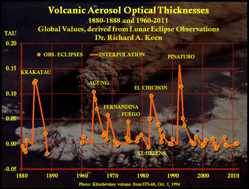
by Dr. Richard Keen, via spaceweather.com (h/t to Leif Svalgaard)
On Sept. 27th, millions of people around the world watched the Moon pass through the shadow of our planet. Most agreed that the lunar eclipse was darker than usual. Little did they know, they were witnessing a sign of global cooling. But only a little.(continued below)

Atmospheric scientist Richard Keen of the University of Colorado explains: “Lunar eclipses tell us a lot about the transparency of Earth’s atmosphere. When the stratosphere is clogged with volcanic ash and other aerosols, lunar eclipses tend to be dark red. On the other hand, when the stratosphere is relatively clear, lunar eclipses are bright orange.”
This is important because the stratosphere affects climate; a clear stratosphere ‘lets the sunshine in’ to warm the Earth below. At a 2008 SORCE conference Keen reported that “The lunar eclipse record indicates a clear stratosphere over the past decade, and that this has contributed about 0.2 degrees to recent warming.”
The eclipse of Sept. 27, 2015, however, was not as bright as recent eclipses. Trained observers in 7 countries estimated that the eclipse was about 0.4 magnitude dimmer than expected, a brightness reduction of about 33 percent.

What happened? “There is a layer of volcanic aerosols in the lower stratosphere,” says Steve Albers of NOAA. “It comes from Chile’s Calbuco volcano, which erupted in April 2015. Six months later, we are still seeing the effects of this material on sunsets in both hemispheres–and it appears to have affected the eclipse as well.”
Volcanic dust in the stratosphere tends to reflect sunlight, thus cooling the Earth below. “In terms of climate, Calbuco’s optical thickness of 0.01 corresponds to a ‘climate forcing’ of 0.2 Watts/m2, or a global cooling of 0.04 degrees C,” says Keen, who emphasizes that this is a very small amount of cooling. For comparison, the eruption of Pinatubo in 1991 produced 0.6 C of cooling and rare July snows at Keen’s mountain home in Colorado.
“I do not anticipate a ‘year without a summer’ from this one!” he says. “It will probably be completely overwhelmed by the warming effects of El Nino now underway in the Pacific.”
This lunar eclipse has allowed Keen measure the smallest amount of volcanic exhaust, and the smallest amount of resultant “global cooling” of all his measurements to date. And that is saying something considering that he has been monitoring lunar eclipses for decades.
“This is indeed the smallest volcanic eruption I’ve ever detected,” says Keen. “It gives me a better idea of the detection capabilities of the system (eclipses plus human observers), so when I go back into the 1800s I can hope to find similarly smallish eruptions in the historical record.”
… volcanoes are going to take blame for the pause…
Until they jack the numbers again…
Ya.
Sanity check: 0.6 C cooling from Pinatubo? In their dreams. 0.6 C is 2/3 of the entire global anomaly from 1850, after all adjustments and tweaks and estimation and guesses applied to the thermometric record. Or did they mean a rate of cooling of 0.6 C per decade, lasting only 1 year and producing a total peak cooling of ~0.06 C (which is arguably moderately defensible, although it is the order of the same amplitude scale as the 2.5, 3.5 and 5.5 year Fourier components in the climate’s natural variation scheme and hence is literally almost invisible in the global anomaly unless you know beforehand where to look. See Willis’ excellent game of “hunt the volcano”. If you can’t find VEI 6 eruptions in the climate record just by looking at the global anomaly, why bother with piddling little VEI 4’s like Calbuco? Seriously folks. VEI is a log scale — this is one hundredth of a “pinatubo”. Admitting that VEI isn’t really the right variable, as different volcanoes at different cone heights and different latitudes with different eruptive chemistry can probably produce very different stratospheric modulation of insolation — still VEI 4 is small enough that empirically it should have an effect utterly, utterly lost in the noise, far less than the 0.1 C of acknowledged probable error in HadCRUT4.
So I’m perfectly happy that they have a good proxy for detecting this, although one would expect that it would show up far more cheaply and easily:
a) In the direct transmittivity measurements being made at Mauna Loa:
http://www.esrl.noaa.gov/gmd/grad/mloapt.html
Whoops, no, guess not. At least I can’t see anything but noise in the 2015 points just like the noise everywhere but in the early 60’s, El Chichon, and Pinatubo. So I guess that the hypothesis that it is affecting well-mixed stratospheric transparency is not validated by a direct measurement of well-mixed stratospheric transparency. Or
b) CERES data. Seriously, why do we bother with these expensive probes if we’re not going to use them to address questions like this. I’m still struggling with the posted fact that CERES is supposedly accurate to only 2% facing sunside and 1% facing the Earth — we spend a gazillion dollars to loft a satellite intended to measure incoming and outgoing full spectrum radiation and the best we can do in accuracy with modern equipment is 1%? And we have no way to calibrate them any better than that built into the instrumentation? But even without being able to set the absolute scale of CERES detection well enough to resolve a radiative imbalance at the TOA, we surely ought to be able to detect any 0.1 W/m^2 modulation of the stratospheric albedo right down to the spectrographic bands involved, or why bother?
I’ve got a nice suggestion for them. Install a set of normalization sources on the surface of the Earth. These should be something like controlled blackbodies radiating at 1500 C or thereabouts with an area of 10 m^2 or whatever is large enough to be directly picked up by CERES through a comparatively small angle as it passes overhead. Mount detectors 30 meters or so above the blackbody (cavity) aperture so that one can directly measure and compare the spectrum at the BOA, compare this measured spectrum to CERES, and BOTH determine the zero of the CERES detector assuming only that its linearity isn’t completely screwed with a signal that swamps the noise AND determine the broadband transmittivity of the atmosphere from bottom to top along the line between source and detector. After all, that’s what one would do on Earth, right? Use a reference source to calibrate. If they didn’t build a precise reference source into CERES itself (again, if not why not?) then provide one on the ground that has other utility.
So anyway, while I agree that they detected something interesting about the atmosphere in the redness of the moon just as I think that the good old Earthlight project was doing a good job with the average albedo of the planet before CERES took over with its unzero’d data, I’d say there is a lot of work to be done before a) claiming that it is due to a volcano (especially when it doesn’t show up as a signal resolvable from noise at Mauna Loa) and b) ANNOUNCING TO THE WORLD that it is from that volcano. Really? You are certain of this how? Could it not be from other things — modulation of other components of the stratosphere or troposphere, for example?
rgb
rgb
What pause? It’s all been swept away by The Ministry of Truth.
How about bouncing lasets off the moon and analyzing the amount of signal loss?
Do this with a bunch of different wavelengths of laser.
Yes, no?
A couple of the Apollo missions left mirrors on the moon. They were used back in the 80’s to accurately measure the distance from the earth to the moon. I don’t know if they were used for anything else after that. You can check with NASA, I’m pretty sure they are still there.
We’ve been bouncing signals off the moon since the 1950s.
There are several satellites which incorporate retroreflectors. Using one of those to measure atmospheric transmission and scattering (at visual wavelengths) is almost a science fair project.
HadCru global temps got exponential boost
http://www.vukcevic.talktalk.net/HC-cor.gif
rgb makes some typically valid points in his typically pithy manner, so I’ll some time out of my busy day (I’m doing dinner tonight – grilled brats) to address some of them. Here goes….
rgb: Sanity check: 0.6 C cooling from Pinatubo?
rk: Yep. But that is the instantaneous cooling at the time of the peak global aerosol optical depth (AOD), calculated from some simple formulas that even James Hansen agrees with. Averaged over a year it gets smaller, and with a minor el Nino in 1992 the net cooling in Roy Spencer’s MSU data is about 0.25C.
rgb: If you can’t find VEI 6 eruptions in the climate record just by looking at the global anomaly, why bother with piddling little VEI 4’s like Calbuco?
rk: The only two VEI 6 eruptions in the past 150 years are Krakatau and Pinatubo, and each dimmed the moon by 100x or more, as did the VEI 4 volcano Agung the VEI 5 el Chichon. Meanwhile the VEI 5 monster Mt. St. Helens had no detectable effect on the moon. Why? Mt. St. Helens was low sulfur magma, and blew horizontally. Two years later, el Chichon blew high sulfur stuff straight up into the stratosphere. So it’s not necessarily how must ash and lava the volcano makes that counts, it’s the amount of sulfur (which makes sulfuric acid haze) blown into the stratosphere that counts (for eclipses and climate).
rgb: one would expect that it would show up far more cheaply and easily in the direct transmittivity measurements being made at Mauna Loa
rk: Eclipses are pre-paid, so Mauna Loa is no way cheaper. Mauna Loa is also a point measurement, and global distributions of volcanic haze are not uniform. the 1963 Agung eclipse shows as much global aerosol as el Chichon in 1982, but in the Mauna Loa record Agung is a mere blip. But a month after Pinatubo went off I was on the Big Island (Mauna Loa) for the solar eclipse, and the local aerosol layer was several times thicker than the globally average 0.15.
rgb: I’d say there is a lot of work to be done before claiming that it is due to a volcano (especially when it doesn’t show up as a signal resolvable from noise at Mauna Loa)
rk: Like Agung, Calbuco’s haze is still concentrated in the southern hemisphere, and like Agung, it won’t show up as well over Hawaii. Another bit of evidence are the bright and lingering volcanic twilights, which have shown up in the southern hemisphere for months and which are now moving north. It was actually Steve Albers’ report of twilights seen from Boulder that got me to look at eclipse reports in more detail. Before that, I was thinking it was just the umbral “Supermoon” effect. But looking at the data (the graph Anthony posted), all of the visual reports near mid-totality were well below the “predicted” curve. I see no need to wait until when, and if, it shows up at Mauna Loa. From previous events, eclipse darkness and enhanced twilights are sufficient evidence of volcanic aerosols.
rgbatduke
calm the ceres was a bargain basement investment. You get what you pay for. Instead think of what we would have had if instead of squandering 63 mil on the rico20……….
Dawn Spacecraft Begins Trek to Asteroid Belt – Space.com
http://www.space.com/4403-dawn-spacecraft-begins-trek-asteroid-b...
Space.com
Sep 27, 2007 – NASA officials set Dawn?s mission cost at $357.5 million excluding the cost of its Delta 2 rocket,
michael duhancik
What do you mean until?
They were Mark, the lads from Mythbusters used them to bust the fake moon landing conspiracy theory, ie if we didn’t go how do we know the co-ordinates of the mirrors? yes i know it’s obviously because the greys told us…
I am very much aware of the reflectors on the moon. That is exactly what I was getting at.
I am not sure why this is a science fair project…personally I never had the equipment when I was in grade school to either send, receive, or analyze a laser beam that would have to a very tightly collimated beam, high powered, and be aimed with extreme precision, and received with instrumentation sensitive enough to discern the needed detail.
In any case, I do not have any of the appropriately aged kids kicking around my shack these days…perhaps CommieBob has some well equipped young lad or lassie wiling to take on the task, and write up the results right here, for us to peruse?
:p)
Here in Papillion Nebraska there was no “blood moon” at all; it was very dark at totality, however. Sky conditions were nearly cloudless and no hint of smoke or other aerosols in the atmosphere at the time of the eclipse. The moon rose pale yellow in color rather than a more orange tone.
It looked the same on the Sherman Summit east of Laramie. I was very disappointed in the lack of blood.
A “bloody” moon was not associated with a lunar eclipse if what I recall from a moon legend that was supposed to forecast a coming disaster?
vukcevic says… volcanoes are going to take blame for the pause…
Well, considering that Calbuco blew up in the 19th year of the Pause, the Pause must have somehow known it was coming! And if a 0.04C volcano can make a pause, whatever it’s pausing can’t be more than 0.04C. That in itself should be an embarassment to the warmers.
But you’re right, do not underestimate the creativity of the warming apologists to make a connection.
Dr. Keen, thanks for your comment.
Apparently 2014–2015 Bárðarbunga’s eruptions released large quantity of SO2 as well.
The 2014–2015 Bárðarbunga-Veiðivötn fissure eruption at Holuhraun produced about 1.5 km3 of lava, making it the largest eruption in Iceland in more than 200 years. Over the course of the eruption, daily volcanic sulfur dioxide (SO2) emissions exceeded daily SO2 emissions from all anthropogenic sources in Europe in 2010 by at least a factor of 3. …………….. we are able to constrain SO2 emission rates to up to 120 kilotons per day (kt/d) during early September 2014, followed by a decrease to 20–60 kt/d between 6 and 22 September 2014, followed by a renewed increase to 60–120 kt/d until the end of September 2014. Based on these fluxes, we estimate that the eruption emitted a total of 2.0 ± 0.6 Tg of SO2.
link to abstract
“The lunar eclipse record indicates a clear stratosphere over the past decade, and that this has contributed about 0.2 degrees to recent warming.”
What recent warming? The past ~2 decades are in “The Pause” the warmistas are so frantically trying to explain. It’s actually cooled slightly. My head hurts …
I mean the warming overall since 1979 (start of the MSU data).
That’s recent to me.
If the clear stratosphere was only over the past decade, it couldn’t have contributed to the “recent” warming because the Pause spans most of the past two decades.
Katherine –
The clear stratosphere has been around since 1995, which is two decades. Most of the “recent warming” happened before that, which is why there’s a pause since.
In reply to rgbatduke. Pinatubo would only affect the NH. Any cooling averaged over the whole planet would be small. Calbuko is SH so no effect in the NH. Also with so few temperature stations in the SH who has data showing what happened?
Not an easy problem and with no data it matters not what analysis you try.
Interesting.
Due to slow hemispheric mixing of the volcanic emissions, and with the eclipse coming very close to the equinox, would it be the case that the atmospheric dimming noted by the brightness of the moon would be less on one hemisphere than the other?
Would this translate into a noticeable variation in the illumination of the hemispheres of the moon during the eclipse?
I just came from spaceweather.com where this is the big story of the day and was going to post it on the tips page. Glad to see it already posted, thanks Dr. S.
Well that explains something. I photographed the April 2014 eclipse, and before this eclipse I checked the exposure settings I had used. I was able to get good photos at ISO-100 last year, but this year I had to bump it up to ISO 400 to 800 to get a similar image. It did subjectively look darker, but I had thought perhaps this eclipse had been deeper into the Umbra than before.
Thanks, Clay.
I experienced the same, more camera gain was required this time.
But what really affected my observation was the thin could cover over south Florida.
The moon was darker for two reasons: it was deeper in the umbra (Supermoon effect), and further darkened by Calbuco. I have a “clear sky” model that predicts the brightness of the moon based on two things: distance from Earth and distance north or south of the umbra’s axis. The purpose of the model is to subtract the purely geometrical effects on brightness from the observed brightness, and the “observed minus calculated” is invariably due to volcanoes. That’s above the uncertainty (noise) level, of course. This one was just at the noise level, but supporting evidence (twilights, etc.) says it’s real.
Fifty-two years ago I had Clay Marley’s experience big time. Using B&W Tri-X film I dutifully used the exposure guide in Sky & Telescope mag for the Dec. 30, 1963 eclipse. Absolutely nothing showed up on the negatives when I got them back. Turns out the eclipse was 1000 times dimmer than “predicted”, thanks to a volcano named Agung earlier that year.
So I recycled those negatives into sun filters, and still use them at solar eclipses.
Clay,
I’m no expert and don’t remember where I read it (maybe Spaceweather.com), but that was the explanation that I read for it appearing darker. This eclipse also coincided with a Supermoon, so was closer to the earth and “deeper” in the shadow (i.e., closer to the earth and less affected by sunlight refracted around the limb of the earth). If so, this would suggest that volcanoes had little to nothing to do with the darker moon.
The article said that it was darker than expected, not darker than the last time.
Why don’t we check to see if the author’s adjusted for the moon’s position before assuming they didn’t?
BTW, the difference mentioned in the article is a lot less than the difference mentioned by Clay.
Good point.
If the moon is closer, which it is during a supermoon, doesn’t that mean less light refracted through the band of atmosphere around the Earth will be able to hit it?
If we have another Pinatubo-class eruption, then there will be a never-ending excuse for the “pause” (assuming it continues).
“Trained visual observers”? Sunspot deja vu. Surely in this day and age we can do better?
Ya think?
“Instrumentation? I don’t need no stinkin’ instrumentation!”
(Hat tip to Blazing Saddles…)
Visual observing is still today a vary valuable tool.
https://www.aavso.org/sites/default/files/publications_files/manual/english_2013/Intro&Contents-2013.pdf
Actually, the “We don’t need no stinking badges!” quote is MUCH older than Blazing Saddles. Try 1948’s “Treasure of the Sierra Madre”.
“Trained visual observers”?
Sure. I could give a long list of important parts of the entire univese that were discovered and measured by those “trained visual observers”. But just a few, from my experience as a meteorological observer for 50= years (and a trained one, too).
1. I’ve seen and reported numerous tornadoes that never showed up on Doppler Radar, and several more non-tornadoes that Doppler Radar said were there.
2. My snowfall measurements made with a 99-cent ruler, along with a yardstick (free from the hardware store) and, once, a high jump measuring stick from a garage sale, are far better than the $20k acoustic depth sensor at a nearby facility.
3. Even the most lavishly funded ASOS weather station needs a human “supplemental observer” to accurately depict the precipitation or cloud type, see an approaching squall line or tornado at the end of the runway, and find glaring errors in the temperature sensor.
4. I’ve discovered and reported a nova, several comet outbursts, a meteor shower, volcanic haze layers, and, of course, tornadoes, all with my little beady eyes, well before the billion buck government funded sensors had a clue.
5. Which have decided more court cases – spectroscopes or visual observers?
6. My eyes tell me much more about someone’s mood than does the smile detector on my point-n-shoot camera.
The human eye is a remarkable sensor (especially when combined with the other input sensors), and in most cases the processer behind it is even more amazing.
“You can observe a lot by watching”
Yogi Berra, 1925-2015.
Yes. I agree. But we need external validation every chance we get. Please see prior responses. I’m getting tired.
Richard Keen
October 6, 2015 at 12:42 pm
“‘Trained visual observers”?
Sure. I could give a long list of important parts of the entire univese that were discovered and measured by those “trained visual observers”. But just a few, from my experience as a meteorological observer for 50= years (and a trained one, too).”
That is because you have keen eyes.
My two-cents: I thought the eclipse was dark. I rated it at 0.5 on the Danjon scale at mid-totality, although I thought the color to be obviously of an orange hue, rather than the scale’s standard “gray or brownish” descriptors. No details were visible with the unaided eye. (Marydel, Delaware; intermittent clouds, but at times clear enough to clearly see the faint stars near the moon with binoculars).
Interestingly the write-up at Spaceweather.com stated that the red-orange hues are due to primarily tropospheric (not stratospheric) refraction of sunlight–essentially, from all the sunsets and sunrises of the world. Occasionally one can see a “turquoise” fringe around the umbra that is supposedly due to stratospheric ozone that preferentially absorbs red light. I am not sure how this fits with your theory. In any event, I saw no hint of the “turquoise” fringe either with my unaided eyes of with my Canon IS binoculars.
Wow. I have nothing but respect for human visual observation. I look through my microscope, I see mites walking around on my grape leaves. It’s the only game in town. No machine can do this.
But consider the sunspot data. It has been revised and revised because, well, is this little speck over here a sunspot or not? There may be machine learning these days capable of parsing this, but only in the last few years.
We need the machines. Not because they are better than us, but because they provide a check on our natural superstitions.
Otherwise it becomes like wine sensory evaluation. Totally subjective, and whoever flails their arms the most and conjures the most effusive prose wins.
Visual sunspot counting is a lot less subjective than you think. Observers with similar telescopes agree pretty much on what the count should be. Different telescopes can be handled by suitable conversion factors determined by comparing observers. And the human eye has not changed over centuries so have constant calibration. Machines are fine, but need be calibrated and do not reach far back in time. The visual determination of light magnitude is also highly reliable and amateurs making visual observations are still contributing to useful science.
Fair enough.
Been thinking that water as a “volcanic aerosol” affects the observed darkness of the moon.It not only scatters as liquid clouds and solid ice, but consistently absorbs in all three phases across the solar spectrum.
“there is good evidence that Max Waldmeier (1948) introduced a weighting of sunspots
716
according to size and complexity in 1947 (section 5.2 of Clette et al. (2014), Svalgaard
717
and Cagnotti (2015)”
Subjectivity.
“Atmospheric scientist Richard Keen of the University of Colorado explains: “During a lunar eclipse, most of the light illuminating the moon passes through the stratosphere where it is reddened by scattering. However, light passing through the upper stratosphere penetrates the ozone layer, which absorbs red light and actually makes the passing light ray bluer.” Sept, 27, 2015 Spaceweather.com
Oops! I guess I misremembered this. Sorry. But still, I would think that it seems “intuitively” more reasonable to reason that the (dense) tropospheric refraction would play a much more dominant role in the color of the umbra than the stratosphere. After all, isn’t this where most of the meterological optics of the twilight plays out?
Yes? Wherever the aerosols are is where the effect is going to play out. The “moon illusion” is the scattering of light through a long low angle trajectory the atmosphere. The moon appears bigger than directly above.
Hard to imagine how to separate the atmospheric layers without satellite “optical thickness” help. Maybe Roy Spencer can do it.
I really dig visual observing. Helps me a lot in getting to where I am going.
Was Tycho Brahe, a visual observer ?? He apparently got a lot of stuff correct.
g
Everyone not blind is a visual observer. Go for it. But our brains are superstition machines. When visual observation is the only game, as it was and possibly still is for sunspots, there you go. When you are talking about “darkness”, this is something that is definitely measurable with instruments. Just take a picture, go to Picassa, and you can dial in any brightness or darkness you like quantitatively. This is homeowner stuff. Serious folks have access to far better.
We need the machine data to cross check our superstitions. This is the nature of science.
Perhaps this is a way to admit cooling while continuing to predict warming.
My feeling is that cosmic rays play onto the observation here and help explain why a relatively small eruption would provide enough aerosols to be cooling effective.
IMHO they should be looking at solar activity vs Cosmic radiation vs stratospheric nucleation.
All said by a retired higher ed facilities manager… am I way off base here Dr Spencer?
Roy,
A Pinatubo-class eruption will also, in a few months, add 5 or 10 years to the statistical “pause”.
BTW, like you, I put “pause” in quotes. Definition of “pause” is a temporary interruption of an ongoing process. In this case the ongoing process – global warming – is so tiny that random events like el Nino and volcanoes can make it appear to disappear. It’s like hiding an ant with a postage stamp. Doesn’t work with a horse.
That puts the lie to the claim that greenhouse gases are the overwhelming cause of “cliamte change”.
Dr. Keen, with all due respect sir, we hope the scenario is global warming.
(What I mean is natural interglacial warming)
Temperature is a function of forcing.
If net forcing decreases, theory says warming will abate.
Not an excuse. Rather it’s exactly how the system works.
Apart from wondering what the SI unit of forcing is; I really wonder what exactly is that function that relates it to Temperature; or is that only verse vicea. ??
Does that function relate my local Temperature to my local forcing; and if not why not.
Why doesn’t my 6PM news give local forcing information; since they do give Temperature.
g
Forcing is usually quoted in power per unit area i.e. Watts per meter squared. Which technically is kilograms per second cubed but that doesn’t make intuitive sense.
You could instead multiply all forcing figures by the area of the earth (510072000 kilometers squared) and get the total delta for the flow rate of energy out of the Earth system, ie Joules per second or Watts.
It does not make physical sense either.
What the heck is a cubic second?
Have you never heard of a third time derivative before?
If it continues, at what point will it cease to be a “pause”?
If we have definite cooling, can this be taken as an end to the pause?
Will it then become a “bifurcated baking”, waiting for the second half?
Some seem to prefer the term “hiatus”. Why is this? Anyone? Anyone? Bueller? (Sorry, I just love Ben Stein is all)
And finally, is there any point at which warmistas will no longer be allowed to dictate the terminology that everyone else must use?
* I lied. My final question is, why are we talking in “quotes”?
Is there a way to get a satellite to constantly record this? It’s would need the equivalent of a ego-stationary orbit.
And I’m sure NASA would love to jump on the idea and get lots of funding for the project.
Not sure what “ego-stationary orbit is” (the smell checker suggest it honest! … I meant “geo-stationary”
I rather like ego stationary.
Yes, it reads almost Mannichaean.
My ego is so big, it keeps me stationary?
A thing is ego-stationary, if no matter how you turn, it’s still facing you. Obviously.
Paul Simon: “I am a rock, I am an island.”
Ego-stationary is an oxymoron !
Sorry gymnosperm, but ego is a monotonically increasing thing.
g
But of course as Willis has already posted – these ‘forcings don’t matter much’ http://wattsupwiththat.com/2015/07/29/why-volcanoes-dont-matter-much/
So perhaps the claims of cooling are a little overdone?
It is also of interest to go to the link in the story: monitoring lunar eclipses http://www.esrl.noaa.gov/gmd/publications/annual_meetings/2015/posters/P-48.pdf
Here is his conclusions
http://www.leif.org/research/Keen-Global-Warming.png
Yeah, if we include one of the most important feedbacks of the most important “ghg” we can compute lots. I would be embarrassed to have been the author of that slide. Neglecting the hole from the iceberg, the Titanic sailed on quite nicely.
The bottom line is that the gsm models do not predict.
Wow Leif,
Is THAT on the NOAA website? I’ll download it, because now that it is published here, I fear that it will not last long…
interesting.
But if you look at the satellite data, all of that 0.25deg C warming occurred in a single isolated step event in and around the 1998 Strong El Nino (which El Nino started in 1997).
This data set does not suggest that CO2 is responsible for any warming in that there is zero first order correlation between temperatures and CO2, and we do not have sufficient data to see whether there may be some 2nd order correlation, but that would appear highly unlikely given that the data strongly suggests a single one off step change coincident upon (but not necessarily caused) by the aforementioned El Nino which El Nino would appear to be of natural origin and not driven by CO2..
This conclusions (ported on the NOAA website) are consistent with the contemporaneous view held in the 1980s, that a ‘polluted’ atmosphere had caused global dimming throughout the late 60s and 70s leading to the cooling which was then observed, and that the subsequent warming being observed in the mid to late 80s was due to the atmosphere being less heavily ‘polluted’ (which was the result of the clean air legislation in the States and Europe kicking in). At this time, China was not the industrial force that it now is, and CO2 was not being cited.
That contemporaneous view was quickly forgotten (some may say air brushed out of history like the global cooling scare that accompanied it) in favour of the hysteria promoted by Hansen (and others of his ilk). Hansen never seemed to accept that the reduction in aerosol emissions leading to a more transparent atmosphere and natural oceanic cycles played a significant role in the late 1980s warming.
The conclusions are based upon a no feedback scenario. If these are a net positive, then one would expect (on his basis) to see more than 0.33 degC of warming by 2100. But of course, if the net feedbacks are negative (as many consider must be the case since the system has never spiralled out of control and appears to self regulate between fairly narrow bounds) then the expected warming would be less than 0.33deg C.
Perhaps the most significant point behind this post is that it clearly shows that the science is not settled, and there is debate as to the extent of climate sensitivity.
I consider that people should take a copy of this and send it to their local political representative, and the department responsible for energy/climate change.
Wow, that is very, very interesting, Lief. One might argue with the extrapolation of current rates — if any of the three different highly reputable groups (that I know of) who are now claiming that they will build a commercial scale exothermic fusion generator in the next 1 to 5 years are correct, we’ll be lucky to top 450 ppm, and if they aren’t it seems likely that a nonlinearity in the form of either continued growth in the rate of CO2 production or the transient collapse of the global economy if draconian measures are taken to limit it will make a linear extension unlikely as well. doesn’t take up a whole lot of room in a table!) wherein all of this is explained? Do real statisticians and mathematical modelers take one look at the political and scientific morass that is climate scientists and just run from the room, screaming, and leave all analysis to people who (with luck) have learned enough elementary statistics to know how to feed data into R and plot a result and not much more? Do error bars even exist any more, or do we just presume that all experimental numbers are infinitely precise and equally infinitely accurate?
This is very much on the low side for no-feedback sensitivity. Most of the spectroscopic line by line or coarse grain approximated computations get a number closer to 1 C, although they make enough assumptions that a range of +/- 0.5 C is probably not crazy and this is inside that range.
There are a bunch of places I don’t quite understand his argument. For one, Mauna Loa has a direct measurement of atmospheric transmittivity over the same period that shows on the one had a much, much larger peak — both El Chichon and Pinatubo reduced the stratospheric broadband transmittivity by ten percent, that is tens of W/m^2 — and an exponential decay constant of transmittivity back to baseline of less than a year so that four years after the events it was basically back to normal. So yes, it has been flat since Pinatubo (call it 1995), but then it was flat from 1986 to 1991 in between the two and it was flat from 1970 through 1981. Note that the strongest warming observable in the land surface records occurred in between 1983 and 2002 (some would argue for a start time even earlier of maybe 1978) right across the two events that he claims should have SUBSTANTIALLY COOLED the planet, while temperatures remained utterly flat across the bulk of the stretch from 1943 through 1978 to 1983 when was almost identical to what it is now.
It is also puzzling that according to his argument, the clear stratosphere we have now should be causing maximum warming rates, where what is observed is the hiatus/pause (at least a substantial reduction in the pre-2000 warming rate, if not the oft-WUWT-claimed zero slope). As far as I can tell from the poster (which is extremely interesting — he uses only MSU tropospheric temperatures, not any of the land surface temperatures for his analysis) he attributes almost all of the warming across this entire interval to ENSO events.
It is this that puzzles me the most. Although it is easy to observe a correlation between strong El Nino events and step jumps in tropospheric temperatures, I have yet to hear a credible explanation for why these jumps occur and stick. So fine, ENSO ventilates a lot of ocean heat (originally, recal, solar energy absorbed into the ocean) into the atmosphere and warms the planet for (again) a transient period. Why does some fraction of this warming stick around? It apparently resets the local equilibrium in some very subtle way.
We are then left with a two distinct problems that Keen doesn’t address, at least not in his poster.
One is response time. If you change the forcing of the atmosphere, especially “suddenly” by means of a volcanic eruption, the system equilibrium is shifted and the system reacts by trying to reach the new equilibrium. The overall transient response has a (spectrum of) lifetime(s), especially given that the forcing itself, while sudden, is not a step function but is itself transient with lifetimes. Fluctuation-dissipation suggests that substantial information could be obtained about the dissipative modes that most strongly contribute to the transient response to the shock. ENSO is basically a slower version of the same thing — it ramps up more smoothly but it still delivers a bolus of energy into the upper troposphere and stratosphere quite rapidly where one would expect it to have a very short residence time, at most a year or two! Keen is apparently neglecting any sort of response time in his analysis and is if anything treating everything but the residence time of volcanic aerosols as Markovian — no-lag response to the slow CO2 forcing (which I think is fine as it varies so slowly that disequilibration likely never occurs, especially with the natural noise bouncing temperatures around well past the point of regression to detailed balance), and — what, exactly, for ENSO events?
This is the other problem. He attributes “57% of the residual variance to ENSO events”. What does this even mean? In particular, what are his assumptions for the lifetime of a pulse of ENSO-mediated warming and how does he justify the apparent permanent (or at least very long lifetime) shift in the local equilibrium that persists long after the forcing ENSO event occurs?
These are serious problems. One can easily imagine two completely distinct resolutions. One is that the atmosphere is disequilibrated by rising CO2 that is increases forcing but also increases the rate of dissipation in the existing dissipative mode (circulation) structure. Then along comes and ENSO and whacks the entire system, causing the dissipative mode structure to reorganize around a new strange attractor with a higher equilibrium set point. Repeat as CO2 climbs. In this picture, ENSO warming is just deferred CO2 driven warming, and he therefore substantially underestimates the climate sensitivity by attributing the warming to ENSO without a comprehensive explanation of why ENSO should warm the planet at all two years after ENSO conditions disappear, producing if anything a pattern of Hurst-Kolmogorov discrete shifts in local SSTs that generally rise.
The other possible resolution is that suggested by Bob Tisdale — that ENSO events cause local reorganization of the patterns of dissipation all by themselves, more or less independent of other forcings, so that El Nino does cause step jumps in temperature by shifting circulation patterns into a new warmer pattern with a long lifetime component or components that remain as residuals after the “burst” effect is going. La Nina events, in contrast, produce cooling reorganizations. There may be some sort of long term secular forcing that favors one over the other to produce long term warming or cooling, or — and it is indeed a scary thought — it could be literally random, or as random as the output from a chaotic system can be, where temperature changes cumulate based on the integrated sum of El Nino steps up and La Nina steps down more or less as a random walk.
It looks like this is more or less what Keen’s graph does — it integrates El Nino minus La Nina as expressed as the Multivariate ENSO index and multiplies the integral by an empirical best-fit slope, adds an offset (always necessary when dealing with anomalies with arbitrary zeros) and subtracts this from “MSU Global Temperatures” (where I’m not quite certain what he means by this) to obtain his final (quite good) fit to the data based on his estimates of aerosol and CO2 and solar forcings.
However, without a model for just how integrated MEI can cause a cumulated long-lifetime warming of a dynamically and continuously heated/cooled atmosphere that should never have a chance to become seriously locally disequilibrated (after all, it heats and cools across some sort of local equilibrium every day and cycles through an entire broad range of this every year) one literally cannot disentangle the two completely distinct explanations above. In one CO2 is the cause of the integration bias. In the other, there is no bias, it is random (or at least, independent of the CO2).
I would conclude by noting that his fits contain a LOT of parameters. At minimum, he has a constant of proportionality for CO2 concentration to (local equilibrium) temperature, solar forcing to temperature, stratospheric transparency to temperature, MEI (integrated?) to temperature, and an offset. Counting them up, he can metaphorically fit the elephant. Less metaphorically, however good his R^2 there is substantial uncertainty in his fit and he (sigh) does not give any error bounds (who does, in this business)? Just a list of numbers. It isn’t a sensitivity of 0.68 C per doubling where both digits are significant within the precision, and he doesn’t give us the (more honest but still dishonest) 0.7 C that would result from rounding a surely irrelevant digit in his answer, and he doesn’t give us the covariance of his five parameter (at least) multivariate linear least squares fit to the MSU (specific!) data, let alone address the uncertainty in the data he fits to and the fact that it disagrees strongly with surface warming over the same interval.
At a guess — just a guess, mind you — since the volcanic forcing, the CO2 forcing, and the ENSO forcing all eyeball out to be moderately to very covariant across the interval being fit, the coefficients associated with his best fit are pretty uncertain, as one can probably increase the CO2 sensitivity (say) to 1 C and still get a decent fit using the remaining parameters, or possibly DECREASE it a bit and still get a decent fit. Sure, maybe not the “best” fit, but just how sharp is the multivariate valley of which the best fit parameters are the minimum? Are we trapped at the bottom of a narrow well, so we should really take his 0.68 C seriously? Or is it more like we are in football stadium, and somewhere out in the middle of the field is a footprint left by a particularly heavy linebacker and we are “stuck” in that as the minimum error for the parameters, only the ground is still oozing back up from the event that created the footprint and tomorrow it might be somewhere else.
Then there is the question — suppose we did exactly the same analysis with HadCRUT4? That gives us a total warming over the same interval of around 0.5 C compared to MSU (RSS?). This is around twice as much, so should we just double 0.7 to 1.4 C per all-feedbacks doubling of CO2 (which is, incidentally, in much better agreement with theoretical computations and other articles I’ve recently read that strongly reduce the role of aerosols in the entire picture of global warming in parallel with (damned confounding covariance!) a reduction in the all-feedbacks CO2-attributable warming? And if we do this, what is the range of probable error?
So yes, a VERY interesting poster, but one that leaves us in a dark and gloomy room where we know little more after looking at it than we did before. We know that IF one uses RSS as a temperature series and IF one does a minimum five parameter fit to it using as inputs four timeseries (only one of which is the measurement of the author of the paper, none of which have displayed uncertainties) then a fit — we aren’t even told that it is the best fit but I certainly hope that it is — has TCS of around 0.7 C per CO2 doubling, not in a no-feedback estimate (he just has this bit plain WRONG) but in an all-feedback estimate, since by omitting any explicit consideration of feedbacks he is rolling the entire feedback response into the one parameter fit on CO2 with the additional assumption of zero lag, and without any statement of error or covariance in the multiparameter fit. We can guess that if we used other global temperature indices, we’d very likely get a very similar pattern of fluctuations but on distinct scales, e.g. HadCRUT4 approximately equal 2x RSS, so that we could guess that TCS is similarly doubled. We can guess that this makes TCS estimated by this method so uncertain as to be very nearly useless, especially when we don’t know if it is 0.7 C plus or minus 1.0C (in which case we might as well have called it 1. C in the first place) and hence 1.4 C plus or minus 2.0C ditto AS WELL as the fact that we have to add the manifest uncertainty caused by the disagreement of the two indices, plus (if we REALLY want to be picky) the uncertainty produced by THEIR never-plotted-except-in-one-case-by-me error bars.
I do sometimes despair. Is this the best work the human species is capable of? Is there a peer reviewed paper that goes with the poster (where there is, I admit, a problem of room to put things, although I think that
rgb
RGB, that had me cheering and my wife wondering what game I was watching. I owe you for the knowledge and wisdom.
rgb, Wow! I’ll address a few of your points, but I really gotta get those brats on the barbie!
rgb: Mauna Loa has a direct measurement of atmospheric transmittivity over the same period that shows on the one had a much, much larger peak — both El Chichon and Pinatubo reduced the stratospheric broadband transmittivity by ten percent, that is tens of W/m^2
rk: Mauna Loa reports the reduction of the direct beam of sunlight. Most of that, say, 10% reduction is scattered out by the haze. But guess what – much of that scatters back down to the ground. After Pinatubo you could see that as a dim sun (yum…) surrounded by a bright milky sky. The net effect is a 10% AOD (direct beam dimming) reduces the radiation reaching the ground by just 2.1 W/m^2 That number is from Hansen and the IPCC, and, yes, there is some useful science from them (if you get it before the summary statements).
rgb: We are then left with a two distinct problems that Keen doesn’t address, at least not in his poster. One is response time.
rk: I’m using annual averages of everything, and assume any response times are less than a year and disappear into the annual average. I did run all this using a variety of tapered lags, but the instantaneous (year long) numbers gave the best correlations.
rgb: It is also puzzling that according to his argument, the clear stratosphere we have now should be causing maximum warming rates, where what is observed is the hiatus
rk: No, the clear stratosphere since 1996 means we should have had the full CO2 warming rate since. And we have. But the full CO2 warming rate is so minuscule – 0.04C/decade – that a single random blip early on (the 1998 Nino) can create a statistical hiatus. There was a recent post on WUWT where some warmer said the hiatus was statistically indistinguishable from the warming trend, meaning the warming trend continues. But we can easily reverse his statement to say the warming trend is statistically indistingishable from zero.
rgb: This is the other problem. He attributes “57% of the residual variance to ENSO events”. What does this even mean?
rk: Simple regression. The whole “model” is a KISS exercise. For volcanoes, CO2, and solar I use the Planck response, i.e., add those forcings into the surface energy balance and recompute using the Stefan-Boltzman Sigma*T^4 equation. No more feedbacks, no clouds, water vapor, or missing heat. And the temperature respons is instantaneous, or at least within a year. Solar drops out because it’s so small.
So I have that volcano-CO2 radiative balance temperature, subtract that from the observed annual MSU temperatures, and get a residual that’s due to everything else. So correlating that with the ENSO MEI index give the 57% correlation. ENSO is not a forcing, but a large part of the internal quasi-random variance after the “external” factors (volcanoes, CO2) are removed.
On my poster which is linked here, I use a 3 parameter model (Volcano, CO2, and ENSO) to reconstruct 36 years of observed MSU temperatures. From the poster:
“A reconstruction of annual temperatures, using only Volcanic and GHG forcing plus el Niño effect = 0.135*MEI, correlates with MSU global temperatures, r = 0.93”
Not bad, methinks, and concludes that volcanoes and greenhouse gases have contributed about equally to the tiny warming over the past 3 decades. On top of that is a random component, mostly thanks to ENSO.
rgb: we aren’t even told that it is the best fit but I certainly hope that it is — has TCS of around 0.7 C per CO2 doubling, not in a no-feedback estimate (he just has this bit plain WRONG)
rk: Note that there’s no timewise trendlines anywhere in the paper. I broke the 34-year record into two halves, one with volcanoes and one without, and compared them. Simple means are less influenced by the exact years of the volcanoes, and are therefore more, ahem, “robust”. I had to get that word in.
And no, WRONG, is IS a no feedback estimate, as described above. Those additional degrees of freedom from variable feedbacks are not there.
rgb: Is this the best work the human species is capable of?
rk: Ohhh… But in terms of climate, maybe so. The models don’t work as well as rolling dice, and guys like Jerome Namias had a much better rationale behind long-range forecasts in the 1950s than anyone does today. Climate is a messy science, like psychology, economics, or astrology. I’m retired, away from university politics and censorship, and happily tinkering with some good data (I know it’s good, because I observed some of it) to show something that looks obvious to me.
“I am putting myself to the fullest possible use, which is all I think that any conscious entity can ever hope to do.”
– HAL 9000
It is not commonly discussed but volcanic eruptions release large amounts of water vapor as well as CO2.
This link:
https://volcanoes.usgs.gov/hazards/gas/
gives example compositions for volcanoes on convergent plates (e.g. the Cascade volcanoes), divergent plates (e.g. Iceland’s volcanoes or those along the Great Rift), and hot spots (Yellowstone, Kilauea). The compositions are strikingly different and some (convergent and divergent plate types) are dominantly water vapor. Pinatubo for instance may have discharged as much as one-half billion tons of water as vapor in the June 15 eruption according to this USGS link:
http://pubs.usgs.gov/pinatubo/self/index.html
If Pinatubo matched the example “convergent plate” volcano, the CO2 release would have been comparatively trivial. In fact the proportion of Sulphur aerosols is much higher. In any case, the point is that in addition to the “cooling effects,” the eruption would also have contributed an amount of energy as volcanic water vapor condensed, releasing the heat of condensation, and that energy is not from the sun, but from the planet itself.
Well rgb, the numbers that one does statistication on, are of necessity infinitely accurate, because there are no statistical algorithms for dealing with variables; on a finite set of exact real numbers (rational or irrational, but not imaginary or complex).
Now those real numbers in the data set don’t necessarily exactly represent anything real; but that does not matter. All the algorithms work on ANY finite set of ANY real numbers.
It matters not whether the numbers represent anything real or not; the algorithms always work and give exact results.
g
That was supposed to say the algorithms work on a finite set of exact real numbers.
Dunno how the editor simply erased some words.
g
So if you point a detector straight up at the top of the troposphere, it registers a net reduction of 10%. But (if I understand you) this does not integrate the multiple scattering from the stratosphere, so at the top of the troposphere the actual flux reduction is much smaller? Because while I’m happy to have the flux reaching the ground be any number you like, I’m not happy unless that number is proportional to the TOT (top of troposphere) net downward directed flux.
I actually agree, for the most part — my own best fits do not use any sort of lag, although when I try to generate a response function to vulcanism (I put a plot I generated across roughly the same time interval in a response somewhere down below) I do fit it to a decaying impulse function. It has little effect, but then, I’m fitting it having already fit HadCRUT4 from 1850 to the present to CO2. I don’t think I showed this fit (which neglects vulcanism altogether), but here is a reasonable version of it:
http://www.phy.duke.edu/~rgb/Toft-CO2-vs-MME.jpg
that includes a comparison with AR5 MME mean from CMIP5. The fit to log CO2 concentration is impressively excellent with only one meaningful parameter which is easily converted into TCS (and the sadly necessary irrelevant parameter that equates the vertical scale of the fit to that of the anomaly).
In this fit I do the opposite to what you do. I assume that CO2 driven warming is the only important factor over the last 165 years, and that volcanoes, ENSOs, PDOs, and so on are just “noise”. As you can see, this assumption does a gangbusters job of fitting the data (for whatever that is worth given the uncertainties and adjustments to the data) over an interval at least 4x longer than you use, and the remaining deviation can be decently approximated with a harmonic correction for which I have and offer no explanation (although plenty of people on the list are eager to suggest one:-).
It is wrong BECAUSE they are not there. Look, let’s just suppose that there is water vapor feedback, but it is (as we both agree) likely to be more or less immediate. The coarse-grain averaged water vapor content of the atmosphere may go up with the similarly coarse-grain averaged temperature as it slowly rises but it isn’t going to go up five years from now in response to an average temperature change this year — the atmosphere constantly maintains a near balance between water vapor in and rainfall out where the short-term variations in this are probably not driven by average temperature per se. where
where  for some unlagged (or lagged by less than a year) feedback constant F, where I should point out that I’m not talking about the integration of coupled ODEs but the shifting equilibrium solution to an implicit ODE that has time constants order of a year or less (so they are irrelevant in a zero lag model). Then when you fit a response to CO2, you are fitting a response to CO2 and all immediate linear feedback to CO2. Leaving out an explicit treatment of water vapor just means you can’t attribute what part of the total goes with what — maybe it is negative feedback from cloud albedo PLUS positive feedback from water vapor PLUS feedback from the albedo change due to reflection from the backs of swans that are mass migrating in response to climate change — we cannot separate it out. It is no longer separable, but leaving out a strongly covariant variable from a fit doesn’t mean that the value of that variable and the causal relationship between the variable and the variable it is covariant with is not implicit in the fit.
So suppose we increase CO2 forcing, but water vapor tracks along with it so that
Don’t feel bad. This is an ongoing problem with the climate record. One cannot really separate out causes in a multivariate model with a lot of covariance. If the unlagged covariance of water vapor and CO2 concentration is large because of immediate, your CO2 only model is a perfect proxy for CO2 plus water vapor feedback. It’s a simple fact of statistical analysis, but one that is frequently ignored.
I encountered this problem all of the time when building predictive models commercially — if a response target is strongly covariant with an input for the wrong reasons it can ruin your whole day — for example if a particular field is only filled in if the targeted variable has a certain value and is otherwise null. The field is just a proxy for the targeted variable and a model that uses it can do an amazing job of predicting a training set, but sadly trial sets and the real world won’t come with the variable filled in. It is in part the reason that correlation is not always causality, except when it is. It is the basis of Bayes’ theorem. I could go on. If the “feedback” from flipping a switch in your basement greenhouse is turning on the lights, you can’t claim that a model between the switch position and plant growth doesn’t have anything to do with the light the plants receive even if you leave “light” out of the model.
That same plot is clearly labelled in the actual graphic “Predicted from Volcanoes, TSI, GHG, MSI” (emphasis yours). You explicitly include a graph of TSI above. Your second figure on the right refers to “All 3: Volcanoes + GHG + Solar”. So I naturally assumed that you used all four quantities in your fit because you explicitly state that you do in the actual graph and spent valuable space on your poster presenting TSI and asserting that you included it in the subtraction that showed a strong correlation with ENSO MEI. you compute your model with the vertical scale of the
  in the RSS anomaly for the purposes of computing a correlation and plotting the two together and so on?
I therefore naturally assumed that you’d need five parameters — the three you acknowledge in your reply, one for solar input (which you apparently omit, which is fine although not at all clear from your then-inconsistent poster) and there MUST be one more — matching the scales of the anomalies. The physical theory for GHG warming requires a two parameter fit to an anomaly, even if you choose to set one of the two arbitrarily (and probably not optimally).
Again, I have exactly the same issues in the fit above — physical theory tells me the probable functional form of the temperature change due to CO2, but I have to match up the scale of my fit function with that of the anomaly (which essentially has an arbitrary zero, unlike an absolute temperature). The price one pays in the fit is one more adjustable parameter, one more degree of freedom. So I still count your number of parameters as four even if you omit TSI (in which case you should definitely fix the figure, don’t you think?).
Do you disagree? If so, how do you align the vertical scale of the
Finally, I’d appreciate any remarks about what you get if you fit e.g. HadCRUT4 as well as (I presume) RSS using exactly the same, hopefully scripted fit procedure. Obviously there is no room on the poster for this, but I’d expect this to be one of the first questions you get asked almost anywhere you present because of the sad fact that people who want to emphasize global WARMING tend to use the surface record(s) like HadCRUT4 or GISS for that purpose while people who want to de-emphasize it use RSS or UAH, because there is almost a factor of 2 scale difference between them across the range of the satellite records. I personally am not asserting that one or the other is “right”, only that a scientifically fair treatment that would properly end up with you being called names by both sides would do both fits and indicate the difference and maybe even use this to establish a (substantial!) range of uncertainty. And don’t worry — 1.4 C is still a very low TCS compared to AR5’s claims.
There is another substantial advantage to doing this. In addition to fitting the exact same interval (where I’m guessing you’ll get almost exactly a factor of 2 difference in the result, as the two datasets are almost exactly a scale factor of two apart) you could do a THIRD fit using your volcano/AOD data against HadCRUT4 or GISS all the way back to Agung (say, 1960). This would substantially increase the time frame you fit (which is always a good thing to do with fitting timeseries and making claims with the result!) and make the fit result less likely to be spurious.
I personally would be very interested in whether or not you can make the same fit coefficients (what the hell, scaled by two or otherwise refit to HadCRUT4 from 1979 through 2015) hindcast HadCRUT4 back to 1960 — you do have a graph in your poster of Tau all the way back to 1960, right? Or fit 1960 to 1980 and then forecast the rest. These are all things I routinely do when building a predictive model, if I can (if I have enough data). Use half for training and half for model validation. If the model built with one half works for the other (or if the model fits to the two halves independently have almost exactly the same best-fit parameters), then we’ll talk about robustness.
BTW, I hope that this discussion isn’t annoying or bothering you. I am obviously very interested in your result, even though I don’t think I believe your estimate for the sensitivity (and wish you had included error bars). But I’m willing to be convinced. I’m tempted to screen scrape your data from the posters and/or sources indicated and try to apply your method to fit HadCRUT4 myself, since I’ve got R-scripts already written and tuned up to do that fit with a single command. Send me your input data and I’ll definitely do it, as that would substantially reduce the energy barrier I’d have to overcome while teaching two courses and grading exams this week…;-) I’m rgb@phy.duke.edu.
rgb
Similar correlation claim can be made for the changes in the earth’s magnetic field. While the CO2 FAILS the PAUSE TEST, the Earth’s own ‘driver’ correlation holds strong !
http://www.vukcevic.talktalk.net//GT-GMF1.gif
As the years went by, 1940’s were corrected downwards, i.e. cooled down else correlation would be even stronger. Earth’s dipole runs about a decade ahead, which would suggest IF there is physical link the mechanism could be related to the delay due to ocean currents’ heat transport from the equatorial to polar regions.
All data are from the NOAA
Why does the El Nino 1997/98 keep global temperatures up?
It didn’t keep them up because the data sets below did show this energy was slowly escaping from the sudden step up.
http://www.woodfortrees.org/plot/hadsst2gl/from:2001/plot/hadsst2gl/from:2001/trend/plot/hadcrut3gl/from:2001/plot/hadcrut3gl/from:2001/trend/plot/rss/from:2001/to:2014.5/trend/plot/uah/from:2001/to:2010/trend
Global temperatures were cooling after the El Nino, but were only slowly cooling years after. If no moderate/strong El Ninos had occurred recently this trend would had continued until back to levels before 1997/98 El Nino. This scientific evidence shows with link below why El Ninos take many years to lose energy once released, not just around the event itself.
The solar connection with ENSO and especially release of energy via El Nino’s are highlighted below.
http://i772.photobucket.com/albums/yy8/SciMattG/SunSpots_v_NINO3.4Minrem_zpsjazoxqcs.png
The solar connection with ENSO and especially release of energy via El Nino’s are highlighted below
Which clearly shows no correlation whatsoever. [I know that you didn’t explicitly claim there was one].
Added the sudden step up.
http://i772.photobucket.com/albums/yy8/SciMattG/RSS%20Global_v1997-01removal_zpszk83g0xi.png
“Which clearly shows no correlation whatsoever. [I know that you didn’t explicitly claim there was one].”
No statistical correlation with solar and ENSO shown, but currently 85.7% chance an El Nino will complete after solar maximum once at least 50% reduced. That percentage is too high to suggest random behavior.
Only time observed El Ninos completed during solar maximum were when the planet was originally cooling significantly. Why the change in behavior between then and the warming period after I don’t know yet?
Why has an strong El Nino never completed during maximum yet?
My reasoning would be because the energy has not built up enough yet in the Tropical ocean upper 300 m to be able to produce one. When one occurs during this period energy is lost to the atmosphere prematurely from the ocean upper 300 m, before it gets chance to build up into a strong El Nino from solar maximum.
No statistical correlation with solar and ENSO shown, but currently 85.7% chance an El Nino will complete after solar maximum once at least 50% reduced. That percentage is too high to suggest random behavior.
Just ‘small number statistics’, thus also not significant. Plus, looks really tortured.
rgb: Do error bars even exist anymore, or do we just presume that all experimental numbers are infinitely precise and equally infinitely accurate?
rk: Not in climate, practically speaking. Oh, people put them on their charts to make the graphics look scientifical, but they are without worth.
Example: Gavin puts +/-0.05C error bars on his global temperature graphs, and a year later “corrects” his data to new values outside of his error bars. This happens repeatedly, and he never admits the irony of it all. So in one swell foop he shows that both his numbers AND their error bars are wrong. Just one example of this found by Steve Goddard at
https://stevengoddard.wordpress.com/2015/09/08/more-detail-on-gavin-hiding-the-hiatus/
Besides, who can measure the temperature in their backyard, or in their bathroom, to +/- 0.05C accuracy, much less than of an entire planet covered with plains, forests, cities, mountains, and oceans. How does Gavin figure he can get the entire Earth to +- 0.05C using thermometers that are +/- 1.00C scattered a few hundred or thousand miles apart, when the temperature across the runway can be 5C higher or lower?
Those error bars are indistinguishable from shinola, and the numbers they should be error barring are scarcely any better. The error bars themselves need error bars that are twice as large.
If you want error bars from me, check out my ancient paper printed on bark some years ago:
Volcanic Aerosols and Lunar Eclipses
RICHARD A. KEEN
Science 2 December 1983: 1011-1013. [DOI:10.1126/science.222.4627.1011]
http://www.sciencemag.org/content/222/4627/1011.abstract
http://www.sciencemag.org/content/222/4627/1011.full.pdf
The estimated error is the scatter in AOD values for those years that have no distinct volcanic events, no more, no less. It’s an eyeball guess. I could pull a Gavin and figure a much tinier formal error bar and actually get it by the reviewers, but I really hate to lie. Besides, that eyeball estimated error seemed good enough for the peer reviewers. Detection of Calbuco peeking just above the error confirms that estimate.
You can look at the chart of observed brightnesses of the eclipse and, seeing that they’re all dimmer than predicted during the middle of the eclipse, deduce that the observers are consistent (not to be confused with accuracy, which requires some indisputable “ground truth” that doesn’t exist).
In a lab class I taught I’d have the 18 students go out to the frisbee field and take sling psychrometer observations of temperature, dew point, etc., The we’d calculate the scatter, standard deviation, and so on to give them an idea of the accuracy, er, consistency, of meteorological measurements. So one class learns that there’s a 3-degree standard error, the next section comes in with 1 degree, and they all learn that meteorological measurements are not infinitely accurate. When I take my regular “official” weather observations, if I read 59 degrees, it’s logged as 59 degrees. I don’t take 18 readings to get an error bar, and except for some physicists who might be weather observers, no one else does, either. Gavin might think it’s accurate to 0.05 degree, but we observers sure don’t.
See, I think you’re a physics prof and actually make precise, accurate, and reproducible measurements of accurately measureable things that lend themselves to error bars. Weather and eclipses don’t do second runs (or 18 runs) for a repeat observations.
Worse, Climate Scientists™ interpolate, extrapolate, fill in the gaps, adjust, homogenize, look for the one tree in a million that says the right thing, and when all else fails, pull some numbers out of their pie exits. Then they’ll censor, sue, investigate, have their political connections intimidate, or ask BO to file RICO charges against those who call them on it.
“People underestimate the power of models. Observational evidence is not very useful.”
— John Mitchell, Chief Scientist UK Met Office & IPCC
In summary, error bars are irrelevant here, since Climate Science™ is better described by Fubars.
I’ll get back to your other questions later, but right now the dog’s barking at a bear and I have to calm things down so I can go to sleep.
I’ll get you that data to play with, along with references.
g’night!
“Just ‘small number statistics’, thus also not significant. Plus, looks really tortured.”
Since 1950 may not be that a long period to justify longer term trends and the data is not tortured.
Sun spots are equally scaled down to fit in the 0-1 range and the same period in full is shown below.
http://i772.photobucket.com/albums/yy8/SciMattG/SunSpots_v_NINO3.4_zpspyacuvw9.png
Compared to originally below with ENSO covering periods with less than 50% SS removed.
http://i772.photobucket.com/albums/yy8/SciMattG/SunSpots_v_NINO3.4Minrem_zpsjazoxqcs.png
Hopefully your dog ate the bear and not the other way around. My dog says to tell you she’s jealous of your dog. She was bred to hunt bear and boar and all she gets to do is chase an occasional squirrel or deer. , and that only if we completely ignore the greater problem of kriging temperatures measured with indifferently located and primitive equipment by untrained observers over 3000 km gaps.
 and get 6.2832 or whatever instead of 6.3. Who takes points off of Gavin’s work, or Hadley CRU’s work, when they commit a sophomoric error in presentations to a scientific and political community with a completely false implication of certain knowledge?
We are in absolute agreement. My words were more like the cry of a Diogenes in the wilderness. HadCRUT4 is my favorite one. It actually comes with a whole vector of error estimates per year and I add ’em up to get the total error bars in the figure above. It may be the only time in your professional career you see HadCRUT4 with the error bars actually on the data points, but — you’re welcome.
They are more conservative than Gavin, at +/- 0.1 C in the contemporary record. I haven’t checked to see if the latest NOAA-adopted shift has exceeded that gap, but in any event the gap between HadCRUT4 and GISS is larger than it already, so humorously, it is close to 95% certain that GISS is wrong (according to HadCRUT4) and vice versa, and I haven’t checked either of them against BEST but I wouldn’t be surprised if it is out of the field of both of them.
But the real humor is in HadCRUT4’s anomaly in the 19th and first half of the 20th century. In 1850, 165 years ago, at a time that Stanley had yet to meet Livingstone and the source of the Nile was a mystery, at a time that roughly half of the continental US was unsettled and extremely dangerous to cross, when the Amazon, Antarctica, central Africa, central Australia, and almost all of Asia away from the coasts were literally terra incognita devoid of all thermometers making anything like systematic measurements, at a time that ships followed a handful of well established, mostly coast-hugging routes across a tiny, pitiful fraction of the 70% of the Earth’s surface that is ocean and measured temperature by doing things like pulling up a bucket of sea water and dunking a thermometer in it or hanging a thermometer in the captain’s cabin and reading it from time to time, HadCRUT4 estimates the total combined error in their anomaly to be (drum roll) 0.3C. Just 3 times the error they acknowledge in numbers measured today with the most modern of electronic instrumentation, automatically read in carefully controlled and precisely located stations, in a grid literally hundreds of times if not thousands of times more dense than in 1850.
Last time I looked, errors in the mean of a series of measurements should scale like at least the square root of the number of independent and identically distributed measurements being made. Of course, it could be much larger, but it is really, really difficult to see how it could be much smaller. So I am forced to conclude that HadCRUT4 only contains 9 times as many contributing stations now than it did in 1850, corresponding in a reduction in expected Gaussian error of
It makes me laugh until my belly hurts so much I want to just plain cry.
It’s almost as amusing at the assertions that we can measure the bulk average temperature of the ocean to depths of 700 m or even 2000 m to 0.01 C all the way back to the 1950s with soundings and more recently a network of floating buoys. Sure we can. But sadly, we cannot measure incoming solar radiation at the top of the atmosphere accurately to within 2 lousy percent.
It’s just sad to see a scientific discipline present curve after curve, to present data points themselves that are clearly the result of a complex and possibly dubious adjustment and averaging process, without any error estimate or bar. It’s Orwellian. It’s just plain wrong. To compound the error, the numbers are often published and reported with two or three more utterly insignificant digits, as in 268.14, not 268. or more likely 2.7 x 10^2. This conveys a completely false sense of our knowledge. I take points off of students’ exams routinely for this kind of nonsense, when they multiply out a number like 2.0 by
Anyway (in the event that you’re still tracking the thread) I really would cherish a copy of your data (so I can apply the approach to HadCRUT4), and hopefully you have my email address for out of band communications. I’ll be out of town this weekend plus (fall break) but by sometime next week I can do it. It shouldn’t take long, as I have R scripts that built/rebuild the figure above, I just have to input your data, change the functions in the NLS code and rerun the the scripts.
rgb
Wow…. just Wow…. that would appear to be a game changer…. and just for more Added Emphasis… WOW…
That’ll be gone within hours
Ahh should maybe have read it all first, rather than just reacting to Leif’s extract… still possibly a lowercase wow……….. is still appropriate, we’ll see what comes of it……..
Are we all aloud to decide which physics to excuse, in making our predictions ??
What if one does a less simple radiative calculation; like one that is closer to reality, and include H2O and clouds, or anything else that we know about.
How much of the 0.12 Deg C arming would that be responsible for.
I’ve seen climate papers that postulated a doubling of atmospheric CO2 abundance, while holding the surface Temperature constant. As I recall, they calculated how much clouds might evaporate or something like that.
Are you actually alloud to do experiments like that where you make up your own rules about what can change, and what can’t ??
g
We are allowed to use the entrails of chickens extracted with a black-handled athame to make predictions. The only two questions are: Will anyone take them seriously? and Will they turn out to be correct?
Well, OK, a third one — suppose nobody takes them seriously but they do turn out to be correct. How many chickens must die before somebody starts to take them seriously?
A slightly less facetious answer might be: Simple (predictive) models, physical or otherwise are often the best. There are a rather large number of very good reasons that this should be so. For example, from the statistical side: Regression gets very, very tired when one tries to fit 10+ variables. The multivariate topology of the fit optimization surface (the error as a function of the fit parameters on an abstract space) can become highly fractal and convoluted, making many/most fit algorithms fail because they rely on being started “close” to the optimum result. Covariant input variables and confounding input variables both create problems (more or less, strongly dependent on the method being used to generate the “prediction”). From the physical side: Parts of the physics may be known only approximately, and badly, or simply not be computable. An example: We do not know and cannot easily compute the “electron hole” associated with two electron anticorrelation in atomic or molecular electronic wavefunctions, and efforts to include it badly or naively can easily make answers worse than just using a simpler mean field approximation. An even better example: The classical physics associated with the molecules in a jar full of air technically involves solving an initial value problem involving order of Avogadro’s number of molecules, which is absurdly impossible. We therefore invent thermodynamics and statistical mechanics to systematically leave physics out. When we are done and have derived or otherwise justified PV = NkT as a pretty darned good macroscopic preditive result that works over a wide range of conditions, we remember that Darn It! We left out the fact that the molecules are quantum mechanical objects and not classical objects — but in the end it didn’t matter, any more than it mattered that we left out nuclear dynamics inside the molecules. Which is another good reason for leaving out physics — it can just plain be irrelevant (but use up valuable and scarce computational resources nevertheless if included anyway). Or, it can be something that accidentally or for good reasons tends to cancel out on average. Thermal fluctuations, for example, can often be omitted because they are as likely to go one way as another. And the list goes on.
In the specific case of the climate, IMO the right way to approach the problem — long, long before building a meso-scale nonlinear chaotic globe-spanning integration of coupled Navier-Stokes equations with umpty inputs including the kitchen sink — is to build simple models such as the two parameter, physically motivated model I display above. The implicit assumption of such a model is “this is the important physics, everything else is unbiased noise irrelevant to the average result” and while success doesn’t prove that this (null) hypothesis is right, failure does prove that it is wrong. So by not failing, one cannot rule out the possibility that CO2 in an unlagged log model is in fact the driver of global average temperatures with everything else being order of 0.1 to 0.2 C “noise” (or at least, a lot less important).
However, there may be many models that would “work” as well or better. The more degrees of freedom you have in your fit, the more things you can wiggle around to improve a fit, and in general, the closer you can get to the thing you are trying to fit even if the parameters being used are completely irrelevant or only accidentally “useful”. My son used to grow a few inches a year. The Dow Jones Industrial Average used to grow a few hundred points in a year. But the DJIA did not cause my son’s growth, and even if I had been able to build a model with a high value of R it would not have proven otherwise. So one does have to worry about “fitting the elephant and making him wiggle his trunk” and so on, and good statistical models will tell you things about how “important” a fit variable is in creating the final fit. Then there is overfitting — fitting a narrow dataset too closely can often result in a model that fails to extrapolate well to a more general data universe.
There are a variety of methods one can use to try to determine the optimal number of variables and so on, but two things stand out. One is the curse of dimensionality — the size of the solution space scales the multidimensional volume, that is to say really really badly when you get out to 100 dimensional models, and the other (connected one) is the curse of not having enough data for the dimensionality of the model you’ve got. If you have a 10 dimensional model with only two values in every dimension, there are 1000 discrete combinations of the inputs. If you have only 10 samples to fit to, you won’t even populate 1% of the cells, on average and even if you are lucky enough to get a “cluster” of sorts in some projective view, you are very unlikely to have enough data to form the correct joint probability distribution in any nontrivial nonseparable model that is worth the trouble of computing a result.
After all, it is better to read the entrails of a single chicken than to slaughter an entire chicken ranch of chickens and read a steaming pile of guts ten feet high. You may or may not be any more accurate with just the one, but you won’t be able to argue that the answer is in the steaming pile somewhere, you just haven’t been able to find it yet… (bring me more chickens!)
This is sadly very close to the state of the GCMs today. And those darned chickens are expensive.
rgb
.
Seems to be some confusion here between volcanic “dust” and volcanic aerosols.
Quite who wrote this is not clear. It seems to be some kind of press release. WUWT shows this post as be “by Dr. Richard Keen” but is clearly is not written by him but simply quoting him.
Yeah, I don’t use the word “dust” for this stuff, either. But some prefer that over “aerosols”, which reminds many of armpit spray. I think of “dust” as dry particles, while “aersols” are liquid droplets of something mixed with H20. In the case of volcanoes, that stuff is sulfur dioxide that joins with water to make sulfuric acid, H2SO4 I believe. But looking in the dictionary, it doesn’t say “dust” is dry. And is something made of a few dozen H20 molecules really a liquid? It can’t flow…
To avoid having to write a paragraph like this every time I talk about these things, I like to use the meteorological term “haze”, which refers to particles and/or droplets of smoke, terpenes, pollen, salt spray, soot, etc. that’s enhance by H20 molecules joining in; and which hinder visibility. That calls it for me.
Thanks for the comment. Dr Keen.
There is also ‘dust’ ie. solid fine particulate matter. It generally falls out rather quickly. IIRC Lacis et al 1993 estimated a couple of months from detailed physical models calibrated against El Chinon observations. Aerosols linger a couple of years or so.
So Dr. Keen. It is a simple exercise using the principle of virtual work, to prove that inside a ” bubble”, there must be an excess pressure over the ambient pressure (outside the water) and that pressure excess is 2t/r where t is the surface tension in newton per meter units, and r is the bubble radius in meter units.
Now that means that it takes an infinite internal pressure to form a bubble that presumably starts out at zero radius. This of course leads to superheating and bumping when boiling clean water, which is why one should never nuke clean water in a microwave.
Now for the life of me, I cannot see any reason why this exact same calculation would prevent a water droplet from forming in the first place, if it has to start from a zero radius.
Ergo, I have always assumed that water requires a finite radius substrate, in order to condense and form a water droplet.
So I don’t see any real difference between a solid substrate (dust) or some other non H2O liquid to give a nucleation substrate to allow the droplet to form without infinite internal pressure.
What is your take on that ??
g
In fact, if you blast a large number of particles of a solid (say basalt) into the atmosphere, they create shade. Solar energy striking them doesn’t reach the surface and is likely to be reemitted from an “advantaged” position, leaving the atmosphere without bothering to warm anything up much. Consider just how thin a sheet of basalt would have to be before you can see through it.
A well posed question.
I have often looked through a piece of glass (microscope slide) covered with a 50 nanometer layer of deposited gold. It reduces visible light about as much as a pair of typical sunglasses, maybe a bit more.
..and I’m not suggesting gold has the same optical properties as basalt, just adding some perspective.
I expect carbon soot to be a lot darker, I just haven’t worked with accurately characterized monolayers of carbon soot. It’s another reason why it should surprise nobody that even the IPCC acknowledge huge uncertainties about aerosols. But hey, wilfull ignorance is better than bliss sometimes. It gives them large uncertainties into which they can then squeeze their CO2 ‘certainties’.
Interesting that he chooses a reaction of 0.04°C per 0.2W/m^2 forcing. This indicates he thinks 5W/m^2 produces 1°C. The direct forcing per doubling of CO2 is the oft quote 3.7 W/m^2 which is typically quoted as a direct effect of 1.2°C, which is 3.08 W/m^2/°C. So his feedback multiplier is 5/3.08 or 1.62x direct forcing… Considerably below the 3x often quoted as an H2O feedback multiplier, but well above the actual effect which is about 0.25x direct (using OHC)
This is great – direct measurements of the clarity of the stratosphere instead of lots of estimates. Of course, the correlation with temperatures is still an estimate as there are other factors included in this metric. Certainly, Willis’ analyses haven’t shown a big enough impact of volcanoes on temperatures to be noted in any climate records so any impact must be rather more nuanced than a straight linkage.
One thing included in this report struck me as quite important: The 10 years (up to 2008) had seen a particularly clear stratosphere – and yet post 1998 El Nino there was actually very little change in temperature. Now, the report here doesn’t say what happened after 2008, but the reason for the reduction in brightness given here is a volcano in April 2015 – i.e. not a long term event and therefore nothing that can be used to “explain” the pause (which is/was around 15-18 years wasn’t it? Depending on data sets). Perhaps someone who has access to the full data on eclipse brightness since 1998 could comment on whether the “pause” does in fact have show correlation with these direct measurements.
Thanks for the link Leif. This is a much lower sensitivity factor than other have calculated – I take it that others people must be using lower estimates/measurements of stratospheric aerosols. How contentious are these estimates? is there more (or less) agreement on these than on temperatures per se?
They can’t be too contentious. I haven’t seen the Sierra Club rummaging through my trash yet.
Maybe they know I have a dog.
Actually, my aerosol AOD numbers are pretty close to Gavin’s and Hansen’s on their web site. Part of the story is I use Roy Spencer’s MSU temperatures, rather than the HCN/GISS/HadCRU numbers, whatever they are.
High icy clouds obscured much of the eclipse where I live unfortunately. I was able to see a sliver of it slowly disappear though.
It’s rare lately to have clear sky with no stratospheric clouds here at the holler back ranch. It will be interesting to see what happens during the next solar minimum.
The current solar maximum isn’t all that much stronger than previous solar minimums.
Much scarier to repeat the dalton minimum over the next few decades, than to experience gradual warming over the next century. Bur here we are on a big detour, not only in science, but in world politics as well. That is the real reason to fear for my grandchildren’s welfare.
By the way , the sunspot number is 15 today after topping 150 last week. We might see a spotless sun tomorrow if nothing comes over the east limb, and the east limb shows little prominence.
http://www.lmsal.com/solarsoft/latest_events/
Dark moon?
Something about this article is making my head explode with dark forebodings.
Is someone in your head? Like this…
No worries. There is no dark side of the moon, really.
It’s all dark.
As a matter of fact…
Glad someone knew.
So…let me get this right….” they were witnessing a sign of global cooling” except that it’s not. “It will probably be completely overwhelmed by the warming effects of El Nino now underway in the Pacific.”
What Keen saw, then, was the level of an ever present negative element of ‘climate forcing’ against the background of an ongoing warming world
Misleading headline, methinks
I know you can’t help yourself, being a village idiot and all that, but the headline at NASA spaceweather should really be the one you are complaining about. My headline is a take off from it.

Of course, by your history of commentary, we know your purpose here really isn’t intended to be anything but derogatory, so I doubt you’ll complain to NASA about it.
Once again VI manages to completely miss the actual content of the article in his desperate attempt to prove that it has nothing to do with the magical CO2 and global warming.
I absolutely AGREE … that your a village idiot !!!!
Just spent the weekend by Calbuco in Puerto Varas. Still smoking and piles of ‘ash’ on some of the sides of the road. I say ‘ash’ because it’s more like piles of dark grey beach sand with large chunks mixed in. The small towns are still hauling tons of it away.
http://climategrog.files.wordpress.com/2014/07/tls_icoads_70s-20s.png
http://climategrog.wordpress.com/2015/01/17/on-determination-of-tropical-feedbacks/
This article also concludes a similar sized warming due to the secondary effects of major volcanoes ( which Chile’s Calbuco was not! ). It shows a total warming of about 0.1deg C from El Chinon and Mt Pinatubo, slightly less than Dr Keen’s 1.2 deg.C.
The whole AGW panic is case of false attribution driven by preconceived conclusions. Lower stratospheric temperature is key to identification of the cause as volcanic.
Hmmm, but what is the cause? The 80s and 90s were in the warming phase of the PDO, so was that secondary warming really volcanically inspired, or would it have happened anyway? Just take away the two volcanic dips, and you might have the natural warming that would have happened anyway.
R
The warming was principally caused by a 5% decrease in cloud cover between 1991-2003 and contributes at least 2/3rds of the observed changes in the satellite record. The boom and bust in LST driven clearly by volcanoes may or may not be the driver, although it does fit temporally. Low latitude volcanoes do seem to induce a zonal state in the climate system (less airmass mixing, possitive AO) while high latitude volcanoes result in the opposite.
Follow the link, there’s a very detailed article.
PDO is N. Pacific “oscillation” not clear what this has to do with 70S-20S. How does PDO affect the stratosphere at just the same time as the eruptions ?!
Wouldn’t it being a supermoon
have anything to do with the darker eclipse?
The brightness of the surface would be the same (it’s still about the same distance from the sun). The larger angular size will cause the overall object to be brighter. Not enough to measure by eye, but it would show up clearly on appropriate instrumentation.
Yes, but I’m more curious about this being a “super earth” solar eclipse from the moon’s perspective. Wouldn’t that account for some darkness?
Incorrect, in a supermoon the moon is closer to the earth and would be less bright as light must be bent further to illuminate it. The supermoon is a cause of decreased brightness although I don’t know if that was accounted for in the article. My guess is no unless otherwise stated.
It depends on the type of Volcano too. Volcanos high in SO2 (Sulphur Dioxide) will have highly reflective aerosols, dusty Volcanos, not as much. The recent eruption was extremely high in SO2.
I wanted to photograph the eclipse and was stunned at how dark it was. Couldn’t take any pictures at all!
The trouble with Keen presentation is that it only allows for the cooling effects of volcanoes. Once the aerosols settle out ( which takes a few years ) the atmosphere would just return to previous levels. This is not in agreement with TLS record. There is a counter effect which causes a rebound to beyond pre-eruption values.
Statospheric ozone may well be the key factor as explained in the linked article.
Global cooling…until those aerosols fall to the surface. They’ll produce warming on ice/snow by affecting the albedo.
Yes, any cooling will be “just from some volcanoes”. Any resulting extra ice melt from the particulates will be the result of “WARMING just like we predicted!”
Only until the next year’s snows cover it.
If one looks at the volcanic aerosol index it is at very low levels which is in contradiction to what this article conveys.
http://icecap.us/images/uploads/OC16.png
The data shows very low volcanic aerosols . Another example of making up the data.
Err, is that optical thickness In the strat or the trop?
Err, is that optical thickness In the strat or the trop?
AOD is usually ( not always ) total column.
Stratospheric.
Volcanic aerosols don’t last long in the Troposphere – they’re taken up by ice crystals and snowflakes and fall to the ground. And optically, very little of the light passing through the troposphere gets to the moon, so adding some aerosol there doesn’t make much difference. The stratosphere, on the other hand, is normally quite clear and aims the sunlight right at the moon. Putting aerosols there does make a difference.
But the index of refraction of the air and the various components thereof must give a certain focal point, and so the position of the moon must matter, at the very least for some wavelengths and to some degree.
Look at the poster. You are plotting things upside down. He is asserting that the “warming” we observed is the dissipation of the COOLING from the two big volcanoes plus the earlier smaller cooling from the early 60’s eruptions, plus a not-explained stationary bump from the (integrated?) MEI, plus CO2 forcing, plus solar variation (which is close enough to zero one could probably have omitted it, but what the heck).
I don’t think he is making up the data. I just think that the 5+ parameter multivariate (non?)linear fit is non-specific enough to drive a truck through, and based on a small mountain of assumptions that each contribute its own small share of a huge cumulative uncertainty. And then, imagine fitting the exact same data with the exact same R call to HadCRUT4 or GISS instead of RSS.
What he has shown is that we know almost nothing about how CO2 TCS, volcanic and other aerosols, the multidecadal oscillations (of which there are several more than just poor old ENSO, which is forced to carry 57% (!) of the burden of explaining global warming in his fit) and solar variation all conspire in a complex system to cause evolution of the climate or a dizzying array of heterodyning timescales. We lack the data to FIGURE OUT much of anything. And remember, this is a comparatively simple “mean field” model compared to the far MORE complex GCMs, which don’t do anywhere nearly as well at fitting the exact same data (either RSS or HadCRUT4, to be frank).
Taken at face value, we could look directly at Mauna Loa transparency and attempt multivariate fits to it across this interval, and use them to try to add at least estimates of global temperature including all-feedback CO2 fit to a log (not linear) temperature model plus this and that. Oh, wait, I did this already:
http://www.phy.duke.edu/~rgb/cCO2-to-T-volcano-recent.jpg
Hmm, not so good. Of course I don’t do solar variation (why include a 0.1% effect that average out very close to zero?) or MEI (I wouldn’t even know HOW to include MEI, or WHY to include MEI, as I have no idea how a transient event like ENSO can cause a “permanent” shift in average global temperature rather than a simple transient one that regresses towards some secular trend, just as volcanic forcing apparently does in my graph). But still, CO2 only works pretty well, as my NONlinear least squares fit using Mauna Loa directly measured top-of-troposphere transparency as a proxy for shows a lousy correlation and response (and, incidentally, suggests a near total short-time insensitivity to solar input variations of as much as 10%). Mind you, I had to make a small volcanic cone’s worth of assumptions to generate this fit, but it does show at least roughly what nonlinear least squares thinks of volcanoes, which is “not zero, but not much”. CO2 only forcing does a remarkable job all by itself, CO2 plus a 67 year harmonic does even better, and CO2 plus a 67 year harmonic plus volcanoes doesn’t actually, really improve anything. It certainly didn’t “take over” from the CO2 to explain 57% of the warming plus the plateau, although with NLS fitting I might not have tested this regime of possible solutions and there might be an attractor there.
rgb
rgb, good to see you around with your usual incisive wisdom.
I have never understood why everyone tries to regress radiative forcings against temperature. ( Even less a bastard mix of near surface land air temps & SST ).
A radiative forcing will primarily cause dT/dt. Assuming a linear climate response the upshot will be and exponential convolution of the forcing. To try to do a direct regression on temp implies near instantaneous equilibration when we are told this will take centuries.
The kind of approach shown here seems more appropriate to the simplistic linear assumptions.
Do you see anything wrong with that ?
Thanks.
https://climategrog.wordpress.com/2015/01/17/on-determination-of-tropical-feedbacks/
Dr. RGB says “ …and CO2 plus a 67 year harmonic plus volcanoes doesn’t actually, really improve anything….”
My spectral analysis (if correct) shows it to be around 54/5 and 68/9 in the summer, while the N. Atlantic is building its heat content (averaging to somewhat misleading AMO 60ish year cycle) while in the winter 68/9 and around 90 years are predominant.
rgb: poor old ENSO, which is forced to carry 57% (!) of the burden of explaining global warming
rk: that’s 57% of the residual, after subtracting out GHG and volcanic aerosols. Those two carry the bulk of the burden; ENSO is a bit of random noise superimposed on the longer term things. And the CO2 and volcanic forcings are not fit to the observed data – the forcing, in Wattes/m2, are converted to delta temperatures using the radiative equilibrium equation, i.e., Stefan-Boltzman. These delta T are compared to the observed temperature with no multiplier feedbacks, except that radiative equilibrium can be considered a feedback. But NO fitting to the observations. So, independent variables are CO2, volcanic optical depth, observed temperatures, and ENSO. Now, the ENSO MEI index is scaled to the residual temperatures, so that’s a scaling variable. ENSO is annual, not cumulative.
Solar does drop out, and you’re right, that’s a bit sly on the summary poster which skipped that step. So here it is: as you noticed, solar is so minuscule that it effectively disappears, so I disappear it.
Counting ’em up, I have CO2 and Volcanoes scaled to temperatures using fundamental physics, so that’s two variables. ENSO/MEI is #3, and the scaling of ENSO is #4. These four variables fit the observed temperatures over n=36 years with r=0.93. Looks good to me, but I can’t run the experiment over again 50 times to see how good it is.
I use MSU, not RSS, satellite temperatures, but they are close and would give similar results. Why would I bother with GISS, CRU, or HCN, just to find out how Gavin’s, Jones’, and Karl’s adjustment algorithms correlate with the forcings? We already know that the NCDC Adjustments to the USHCN temperature data set correlate with CO2 levels with R2 = 99%
or https://stevengoddard.wordpress.com/tracking-us-temperature-fraud/
That’s the Adjustments, aka “Corrections”, to the observed data. NOT the observed data!
I doubt volcanoes could add much to that 99% correlation.
Ummm… How does a graph that goes to 2012 show that an observation from 2015 is made up?
Also, Calbuco’s aerosol optical thickness is 0.01, about the size of some of those other bumps you call “very low volcanic aerosols”.
And el Chichon is misspelled.
And the Soufriere event in 2007, which shows up on SAGE and during an eclipse that year, is not on the graph.
Finally, no way Mt. St. Helens in 1980 caused that big bump in 1982-83.
Leslie
Very good point. It would be closer in and deeper into the umbric cone. This data needs ‘bias correction’ if it is to be taken as measurement of AOD.
Salvatore Del Prete October 6, 2015 at 9:15 am
Thanks for the graph. What is probably the key point there is the base line. not the peaks. Note how that late 20th c. had a steady baseline AOD since Mt P. cleared up it is effectively zero baseline.
Bias correction? Has it.
The author’s seem to be assuming that 100% of the atmospheric dimming is being caused by aerosols, and that 100% of those aerosols can be attributed to one volcano.
I’d like to see some justification for both of those assumptions.
Simplified assumptions seems to be endemic in the climate community. What about changes in water vapor? Red is the first color filtered out by water. Would not an El Nino be expected to increase water vapor in the atmosphere? A little negative feedback?
No, the author – that’s me – is not assuming that 100% of the atmospheric dimming is being caused by aerosols, but is calculating a “dimming” that can be traced to the Calbuco volcano. There’s gobs of dimming in the atmosphere, some of it by thin air itself. But in the stratosphere, which eclipse observations concentrate on, most of the dimming is from volcanoes. All of the sudden, short-lived bumps in the aerosol recrod can be attributed to volcanoes. In this case, the aerosol patch can be traced back to Calbuco by piecing together other observations, like twilight reports.
Sometimes the culprit volcano is not exactly known, especially if there’s several moderate eruptions around the time of a moderately dark eclipse. On the other hand, in early 1982, a few months before el Chichon, there was a widely observed “mystery cloud” whose source eluded blame for many years. I think it turned out to be some remote volcano in the Andes.
Enormously interesting. You are seriously tempting me to reconsider volcanoes as a possible factor in a good fit, although I have to say that it bothers me that you can have “mystery clouds”. Perhaps a better way to put it is that I am starting to think that specific volcanoes are impossible to model well enough to predict their effect on the stratosphere, but that your measurements of stratospheric opacity tell you precisely the thing that you would have wanted to know about volcanic input anyway, and is what one should use to build the models. One shouldn’t be playing “hunt the volcanoes” (a game that shows that one cannot really look at the thermal record and identify even large volcanoes unless you know just where to look AND they turned out to have a significant effect, where sometimes small volcanoes have a large effect and large ones have a small effect but the stratosphere tells all of asked via eclipses, without naming (or requiring) names.
I’d love a dataset back as far as you have one (maybe the one in your poster at the bottom, although I don’t know what “tau” is).
rgb
Hey rgb,
You’re starting to think like me now! I’m an operational meteorologist at heart – a field meteorologist in the Army, later a storm & tornado forecaster & chaser, and a NWS weather observer for 30+ years (every day). In all these endeavors you make the absolute best observation you can and work with those numbers. There’s not much point worrying about the formal standard error of the observation, since it’s the observation that affects your plan of action, not the probable error.
I’ve known guys who died because of bad data somewhere along the way – from a misaimed 105 howitzer to a misjudged tornado. Better data would have changed the outcome, but a precise standard error would not.
You nailed it – the goal of what I’m doing (besides watching eclipses, a worthwhile pastime) is to get a centuries-long time series of volcanic aerosols in the stratosphere. It is climatologically important. As you say, “measurements of stratospheric opacity tell you precisely the thing that you would have wanted to know about volcanic input anyway, and is what one should use to build the models”. Couldn’t say it better myself. Curiously, the eye and the sun have similar spectral curves, and the amount of dimming of the moon (seen by eye) is directly related to amount of dimming of sunlight heating the ground (or top of troposphere).
“Playing hunt the volcanoes” isn’t bad, either, although it’s not the main point. Identifying a blip is interesting and may confirm the volcanic reality of the event, which I think the supporting evidence of Calbuco has done. It tells me that the calculated dimming of the eclipse, and amount of volcanic aerosols, is real and due to a specific event, and not just a statistical bump. Putting all the volcanoes together – el Chichon had more sulfur than the larger Mt. St. Helens eruption, for example – can tell the geologists something. Knowing that Tambora threw up XX times as much SO2 as did Krakatau may interest lots of geophysical types.
Tau is the Greek letter used to label the vertical Aerosol Optical Depth (AOD), or optical thickness of the layer. Tau in astronomy is a measure of optical depth, or how much sunlight cannot penetrate the atmosphere (Wikipedia).
When modelers add volcanoes to their GCMs, they throw in the tau.