This is a guest essay by Mike Jonas, part 1 of 4
Introduction
The aim of this article is to provide simple mathematical formulae that can be used to calculate the carbon dioxide (CO2) contribution to global temperature change, as represented in the computer climate models.
This article is the first in a series of four articles. Its purpose is to establish and verify the formulae, so unfortunately it is quite long and there’s a fair amount of maths in it. Parts 2 and 3 simply apply the formulae established in Part 1, and hopefully will be a lot easier to follow. Part 4 enters into further discussion. All workings and data are supplied in spreadsheets. In fact one aim is to allow users to play with the formulae in the spreadsheets.
Please note : In this article, all temperatures referred to are deg C anomalies unless otherwise stated.
Global Temperature Prediction
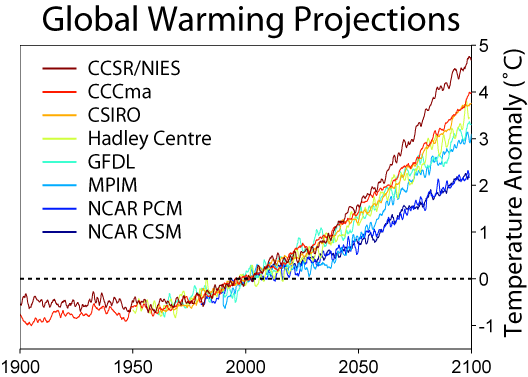
The climate model predictions of global temperature show on average a very slightly accelerating increase between +2 and +5 deg C by 2100:

We can be confident that all of this predicted temperature increase in the models is caused by CO2, because Skeptical Science (SkS) [6], following a discussion of CO2 radiative forcing, says :
Humans cause numerous other radiative forcings, both positive (e.g. other greenhouse gases) and negative (e.g. sulfate aerosols which block sunlight). Fortunately, the negative and positive forcings are roughly equal and cancel each other out, and the natural forcings over the past half century have also been approximately zero (Meehl 2004), so the radiative forcing from CO2 alone gives us a good estimate as to how much we expect to see the Earth’s surface temperature change.
[my emphasis]
So, if we can identify how much of the global temperature change over the years from 1850 to present was contributed by CO2, then we can deduce how much of the temperature change was not. ie,
T = Tc + Tn
where
T is temperature.
Tc is the cumulative net contribution to temperature from CO2. “CO2” refers to all CO2, there is no distinction between man-made and natural CO2.
Tn is the non-CO2 temperature contribution.
Obviously, all feedbacks to CO2 warming (changes which occur because the CO2 warmed) must be included in Tc.
CO2 Data
The Denning Research Group [4] helpfully provide an emissions calculator, which shows CO2 levels and the estimated future temperature change that it causes under “Business as usual” (zero emission cuts) :

Cross-checking the future warming in this graph against Figure 1, the CO2 warming from 2020-2100 is just under 3.5 deg C compared with about 3.25 deg C model average in Figure 1. That seems close enough for reliable use here. But data going back to at least 1850 is still needed.
There is World Resources Institute (WRI) CO2 data from 1750 to present [3], and CO2 data measured at Mauna Loa from 1960 to present [5]. Together with the Denning “Business as usual” CO2 predictions above, the CO2 concentration from 1750 to 2100 is as follows :

For dates covered by more than one series, the Mauna Loa measured data will be preferred, then the WRI data.
Because the “pre-industrial” CO2 is put at 280ppm [6], and the data points in the above graph before 1800 are all very close to 280ppm, a constant level of 280ppm will be assumed before 1800.
CO2 Contribution
The only information still needed is the CO2-caused warming before about 1990.
A method for calculating the temperature contribution by CO2 is given by SkS in [6] :
dF = 5.35 ln(C/Co)
Where ‘dF’ is the radiative forcing in Watts per square meter, ‘C’ is the concentration of atmospheric CO2, and ‘Co’ is the reference CO2 concentration. Normally the value of Co is chosen at the pre-industrial concentration of 280 ppmv.
dT = λ*dF
Where ‘dT’ is the change in the Earth’s average surface temperature, ‘λ’ is the climate sensitivity, usually with units in Kelvin or degrees Celsius per Watts per square meter (°C/[W/m2]), and ‘dF’ is the radiative forcing.
So now to calculate the change in temperature, we just need to know the climate sensitivity. Studies have given a possible range of values of 2-4.5°C warming for a doubling of CO2 (IPCC 2007). Using these values it’s a simple task to put the climate sensitivity into the units we need, using the formulas above:
λ = dT/dF = dT/(5.35 * ln[2])= [2 to 4.5°C]/3.7 = 0.54 to 1.2°C/(W/m2)
Using this range of possible climate sensitivity values, we can plug λ into the formulas above and calculate the expected temperature change. The atmospheric CO2 concentration as of 2010 is about 390 ppmv. This gives us the value for ‘C’, and for ‘Co’ we’ll use the pre-industrial value of 280 ppmv.
dT = λ*dF = λ * 5.35 * ln(390/280) = 1.8 * λ
Plugging in our possible climate sensitivity values, this gives us an expected surface temperature change of about 1–2.2°C of global warming, with a most likely value of 1.4°C. However, this tells us the equilibrium temperature. In reality it takes a long time to heat up the oceans due to their thermal inertia. For this reason there is currently a planetary energy imbalance, and the surface has only warmed about 0.8°C. In other words, even if we were to immediately stop adding CO2 to the atmosphere, the planet would warm another ~0.6°C until it reached this new equilibrium state (confirmed by Hansen 2005). This is referred to as the ‘warming in the pipeline’.
Unfortunately, not enough exact parameters are given to allow the temperature contribution by CO2 to be calculated completely, because the effect of ocean thermal inertia has not been fully quantified. But it should be reasonable to derive the actual CO2 contribution by fitting the above formulae to the known data and to the climate model predictions.
The net radiation caused by CO2 is the downward infra-red radiation (IR) as described by SkS, less the upward IR from the CO2 warming already in the system (CWIS). This upward IR will be proportional to the fourth power of the absolute (deg K) value of CWIS [9]. The net effect of CO2 on IR is therefore given by :
Rcy = 5.35 * ln(Cy/C0) – j * ((T0+Tcy-1)^4 – T0^4)
where
Rcy is the net downward IR from CO2 in year y.
Cy is the ppm CO2 concentration (C) in year y.
C0 is the pre-industrial CO2 concentration, ie. 280ppm.
j is a factor to be determined.
T0 is the base temperature (deg K) associated with C0.
Tcy is the cumulative CO2 contribution to temperature (Tc) at end year y, ie, CWIS.
SkS [6] says “it takes a long time to heat up the oceans due to their thermal inertia”. On this basis, CWIS is presumably in some ocean upper layer.
For a doubling of CO2, in the absence of other natural factors, the equilibrium temperature increase using the SkS formula is 5.35 * ln(2) * λ where λ = 3.2/3.7 (assuming a mid-range equilibrium climate sensitivity (ECS) of 3.2).
At equilibrium, Rc = 0. For ECS = 3.2, j can therefore be determined from
0 = 5.35 * ln(2) – j * ((T0+3.2)^4 – T0^4)
hence
j = (5.35 * ln(2)) / ((T0+3.2)^4 – T0^4)
Because “the natural forcings over the past half century have also been approximately zero” [6], the SST should be a reasonably good guide to CWIS. The global average SST 1981 to 2006 was 291.76 deg K [8]. Subtracting the year 1993 Tc of 0.7 (from the Denning data [4]) gives T0=291 deg K. Hence j = (5.35 * ln(2)) / ((291+3.2)^4 – 291^4) = 1.16E-8 (ie. 1.16 * 10^-8, or 0.0000000116).
Using the formula
δTcy = k * Rcy
where
δTcy is the increase (deg C) in CWIS in year y.
k is the one-year impact on temperature per unit of net downward IR.
the value of k can be found which gives a future temperature increase matching that of the climate models, ie. 3.25 deg C from 2020 to 2100. A reasonability check is that the result should closely match but be slightly lower than the Denning warming calculation in Figure 2 (lower graph) (slightly lower because target is 3.25 deg C not 3.5) …..

….. it does, for k = 0.02611 (the graph for 3.5 deg C is also shown in [7]). [Note that the calculated warming is “anchored” at 1750 T=0, and that the shape is determined only by the formula so there is no guarantee that the 2020 and 2100 temperatures will be close to the Denning temperatures. ie, this is a genuine test.].
Note: At this rate, global temperature takes 52 years to get 80% of the way to equilibrium (as in “equilibrium climate sensitivity”), 75 years to reach 90%, 97 years to reach 95%, 148 years to reach 99%.
The above formula can therefore reliably be used for CO2’s contribution to global temperature since 1750.
1850 to 2100
The above formulae can now be applied to the period 1850 – 2100, to see how much has been and will be contributed to temperature by CO2.
For temperature data 1850 to present, Hadcrut4 global temperature [1] is used. For future temperatures, the formula warming (as in Figure 4) is used.

Applying the above formulae shows the contributions to temperature by CO2 and by other factors :

As expected,
· the dominant contribution is from CO2,
· other factors contribute the inter-annual “wiggles” and virtually nothing else.
Note : The contribution to global temperature by CO2 is only man-made to the extent that the CO2 is man-made. As stated earlier, no distinction is made between man-made CO2 and natural CO2. Obviously, all pre-industrial CO2 was in fact natural. Similarly, for the non-CO2 contribution, no distinction is made between natural factors and non-CO2 man-made factors (such as land-clearing, for example), but the non-CO2 factors are thought to be predominantly natural. The feedbacks from the CO2 warming as claimed by the IPCC (eg. water vapour, clouds) are included in the CO2 contribution above.
Conclusion
The picture of global temperature and its drivers as presented by the IPCC and the computer models is one in which CO2 has been the dominant factor since the start of the industrial age, and natural factors have had minimal impact.
This picture is endorsed by organisations such as SkS and Denning. Using formulae derived from SkS, Denning and normal physics, this picture is now represented here using simple mathematical formulae that can be incorporated into a normal spreadsheet.
Anyone with access to a spreadsheet will be able to work with these formulae. It has been demonstrated above that the picture they paint is a reasonable representation of the CO2 calculations in the computer models.
The next articles in this series will look at applications of these formulae.
Footnote
It is important to recognise that the formulae used here represent the internal workings of the climate models. There is no “climate denial” here, because the whole series of articles is based on the premise that the climate computer models are correct, using the mid-range ECS of 3.2.
See spreadsheet “Part1” [7] for the above calculations.
Mike Jonas (MA Maths Oxford UK) retired some years ago after nearly 40 years in I.T.
References
[1] Hadley Centre Hadcrut4 Global Temperature data http://www.metoffice.gov.uk/hadobs/hadcrut4/data/current/time_series/HadCRUT.4.3.0.0.annual_ns_avg.txt (Downloaded 20/5/2015)
[2] Climate model predictions from http://upload.wikimedia.org/wikipedia/commons/a/aa/Global_Warming_Predictions.png (Downloaded 20/5/2015) Note: Wikipedia is an unreliable source for contentious issues, but for factual information such as the output of computer models, and in the context for which it is being used here, it should be OK.
[3] CO2 data from 1750 to date is from World Resources Institute http://powerpoints.wri.org/climate/sld001.htm (Downloaded 20/5/2015. Digitised using xyExtract v5.1 (2011) by Wilton P Silva)
[4] Emissions calculator from Denning Research Group at Colorado State University http://biocycle.atmos.colostate.edu/shiny/emissions/ using no emissions cuts, ie, “Business as usual”. (Downloaded 20/5/2015. Digitised using xyExtract v5.1 (2011) by Wilton P Silva)
[5] Mauna Loa CO2 data from http://scrippsco2.ucsd.edu/data/flask_co2_and_isotopic/monthly_co2/monthly_mlf.csv (Downloaded 27/2/2012)
[6] Skeptical Science 3 Sep 2010 http://www.skepticalscience.com/Quantifying-the-human-contribution-to-global-warming.html (As accessed 20/5/2012).
[7] Spreadsheet “Part1” with all data and workings . Part1 (Excel .xlsx spreadsheet)
[8] Spreadsheet “SST” SST (Excel .xlsx spreadsheet)
[9] Stefan-Boltzmann law. See http://hyperphysics.phy-astr.gsu.edu/hbase/thermo/stefan.html
Abbreviations
AR4 – (Fourth IPCC report)
AR5 – (Fifth IPCC report)
CO2 – Carbon Dioxide
CWIS – CO2 warming already in the system
ECS – Equilibrium Climate Sensitivity
IPCC – Intergovernmental Panel on Climate Change
IR – Infra-red (Radiation)
LIA – Little Ice Age
MWP – Medieval Warming Period
SKS – Skeptical Science (skepticalscience.com)
WRI – World Resources Institute
“We can be confident that all of this predicted temperature increase in the models is caused by CO2, because Skeptical Science (SkS) [6], following a discussion of CO2 radiative forcing, says :
Wrong.
You are looking at both history and future projections.
If you want to know what FORCINGS drove the model, you cannot and should not rely on SKs
GO TO THE SOURCE.
The forcing files are available for all CMIP experiements.. THAT is the proper source. not Sks.
science 101.. Primary sources. USE THEM.
Hi Steven – Everything cross-checks. The mid-range models exactly match the predictions from the mid-range ECS on their own. Bar a few small wiggles, the past 150 years of actual temperatures exactly match the application of the mid-range ECS on its own (Figure 6). In other words, the past and the future both match exactly the supposed effects of CO2, assuming the mid-range ECS, plus nothing else. The forcings you talk about are all built into this process, IOW they are all built into the ECS. By using the ECS, I am in fact using them.
Which means these effects (presumed to be anthropogenic in origin) fall within natural variability …as best as one can calculate.
Mike: FWIW, I don’t trust SKS to accurately report consensus climate science, so it will be difficult to trust your derivative work. I agree with Mosher, go to the original sources.
You are using a formula with values derived from the assumption that all observed warming is from CO2. That means the results will absolutely match all data that went into the calculation of that value.
It is similar to tricks used to compress image data in a “lossy” manner.
Depending on when you calculated the ECS value you can get different expected curves that will fit the past data and, due to the dependence of future temps on current and past temps, be reasonably assured of a trend that will appear to fit for at least a couple of decades.
I’m also not convinced that there aren’t naturally sources of warming. 20th century solar activity, alone, was quite different than from the 19th century, and no one really agrees on what the effects would have been (more/less cloud nucleation? more/less wind? altered wind/ocean currents? etc…).
And, of course, the other data assumption is the CO2 levels themselves, but there is little we can do about that.
[snip]
[ Until you start providing links and description, you don’t get to simply yell WRONG here anymore. Step up – Anthony]
It depends on what the author’s purpose is, which we do not yet know (at least I don’t, since make no clairvoyancy claims). Lewis and Curry (2014) used central AR5 values (even though several have since been ‘improved’ ) to show that the likeliest ECS must be at the low end of the stated AR5 range. A rather nice ‘Perry Mason’ paper sticking it to AR5, yet also criticized for not using the newest estimates–which would have defeated the purpose. Maybe this is similar, in which case your point is not just irrelevant, but also wrong. Why not have the patience to find out what the purpose here is?
Sketchy Science is what the shill site “Skeptical science” does. It poses as realist, but is actually designed to twist the real science that disproves the Global Warming Claims and make it look stupid or impotent. Find the real thing at WattsUpWith That.com
So many assumptions, so little time. In the end, reality shows it is wrong.
Yeah, Bruce, i don’t spend too much time here at watts, but i must say this is the most delusional posting that i’ve seen here in a long while. I do wish anthony would be more careful about what’s being posted here…
Guys, get a grip. This is establishing what the SkS models say. It’s not saying those models are right.
Agreed, the physics of a specific glibal ti Co2 interaction aught to be well understood by now, its what is not well understood which intrigues the most. There could be dozens of interactions which are not well understood driving climate in spite of C02 forcing. And we may have physics revise the math behind the radiative properties of C02 before long.
Well done looking forward to the series.
So the question becomes what is ECS value? If doubling CO2 will give us 1-1.7 C increase in temperature how do they get to 3.2? Feedbacks? Which ones and where is the data?
Thanks for the article. I’m looking forward to the next 3 parts.
I have strong objections on labeling the RCP8.5 scenario as “business as usual”. RCP8.5 is a worst case scenario similar to SRES A1FI. Using the real busines as usual model SRES A1B with a climate sentitivity of 1.3 yields this: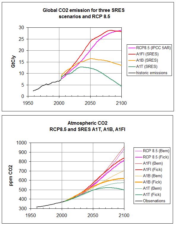
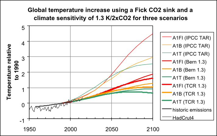
With this temperature calculation:
So only a one degree rise after 1990
Hans Erren,
You are absolutely right. RCP8.5 is a fantasy. The path we are on will take us somewhere between RCP4.5 and RCP6, unless there are breakthroughs in non-fossil energy (as, of course, there will be).
RCP8.5 isn’t a fantasy, it is a scenario based on clear assumptions, no more no less. It doesn’t claim to forecast what might or mightn’t happen, it is a projection that “corresponds to a high greenhouse gas emissions pathway compared to the scenario literature .., and hence also to the upper bound of the RCPs”.
HAS, all scenarios are science fiction the underlying assumption of A2 is increasing poverty combined with extreme population growth. That’s not business as usual for India nor China.
Hans
You miss my point.
The scenarios are no more than the product of their assumptions. Discuss the assumptions and the ways they have been projected into the future by all means, but don’t expect them to give a realistic view of the future unless the assumptions align with what is happening and the methods of projection valid (which as you note they don’t).
The point of criticism is the people that take the scenario and ascribe to it more meaning than it has – claiming for it a realistic view of the future usually under cover of calling RCP8.5 “business as usual”.
I should add that that follows through to the GCMs that are again basically complex projections rather than forecasts, and the RCPs are just one of the assumptions made to form those projections.
GCMs only become problematic when people start saying that their output is the way the world will be (and suggesting their range of outputs are “likely” for example as AR5 WG1 did).
But as you know CO2 can’t produce warming can it! And most of the CO2 came from warming oceans and that has stopped!
Sorry to post off topic, but everyone has to read this. That man Wadhams has completely lost it now!
http://www.telegraph.co.uk/news/earth/environment/globalwarming/11762680/Three-scientists-investigating-melting-Arctic-ice-may-have-been-assassinated-professor-claims.html
And yet, the alarmists are known to continually accuse “climate deniers” of adhering to conspiracy theories.
Micheal Mann’s depression deepened on reading this. He especially felt low about the report on the lady who was in the house when that one guy fell down the stairs claiming that homicide was preposterous. But back to the math at hand!
Also in The Times today, there is an article on the NOAA claim that this is the going to be the hottest year on record, referencing Mann’s latest paper in which he claims we are all going to hell in a hand cart, even with a two degree temperature rise. At that temperature, Mann et al claim a sea level rise of 10ft in 50 years. They also state that CO2 is a ‘tight control knob on global climate’, but they are not claiming that Big Oil is trying to assassinate them, so I guess that they haven’t totally flipped (yet).
I’m dealing with second hand information, so it’s hard to tell how accurate, but according to accounts Giles ran into a small delivery truck, the truck did not run into her. Laxon fell down a flight of stairs at a New Years party and died of a brain hemorrhage.
If this was murder then this is the most clever and skilled assassin in history to have multiple cases where the victim initiates the final sequence leading to death.
They are super ninja turbo charged oil fed murdering assassins that use vulcan mind meld to steer their victims to their demise! They throw Neon bright spinney star like thoughts of death right out of their foreheads!
Easy. Just spike the drinks with heavily magnetized rare earth metals. Person runs into truck because its largely metal. Person falls down stairs because a strange delivery consisting of a blob of metal was left at the bottom of steep stairs. Man struck by lightning because of the metal inside him. I totally buy this (sarc).
In fairness he has a point.
Nobody ever has an accident on a bicycle without there being nefarious causes.
Motorway bumps are unheard of ever. And he probably would have died if he hadn’t had that covert advanced automobile training with MI6 (shh).
And the guy who was hit by lightning was clearly attacked with a CIA/Exxon space Tesla Ray.
Lewandowsky can explain why you’re being irrational in doubting the great scientist.
Arranging for someone to be struck by lightning is a neat trick. Who would ever suspect it was murder?
It just shows that the conspiracy goes right to the top.
Interesting, but unlikely to be a coincidence.
There may be an important common element, which I am very familiar with.
I often come across something in a data file, and however unlikely when it confirms my expectations, I wander down the road oblivious of the surroundings, unable to get it out of my head until I can glimpse some kind of resolution.
These scientists died in early months of 2013, while Arctic Sea ice extent in the late 2012 hit new low.
http://ocean.dmi.dk/arctic/plots/icecover/icecover_current_new.png
All three were very intelligent highly educated people, I suspect they knew perfectly well that this could not have been consequence of the CO2; but what is it and why?
Lack of concentration while riding a bike even for few seconds in London traffic, or coming down stairs (I did it once, had bruised ‘lower back’ for months, my wife see only funny side of it). Going to a UK hospital on Sunday, let alone New Years day with a life threatening injury, a very slim chance of recovery. In the third case could be simply carelessness and ignorance of the elements by walking in a thunderstorm while the mind is preoccupied by some other matter.
Professor Peter Wadhams you are wrong, not succession of assassinations, as your own case confirms. Of course you wouldn’t be also loosing concentration while driving and daydreaming about “ that the North Pole will be exposed (no ice) this summer – it’s not happened before” as you claimed some years ago, or some other nonsense, but for some reason a crazy lorry driver didn’t like your climate politics.
It is entertaining to see so much math, when some of the underlying initial assumptions are completely fabricated. I have seen nothing which would indicate that carbon dioxide was a specific steady-state level from 1750 to about 1900. The published numbers from that time were all over the place, depending on where the air samples were taken. The numbers being used here are taken from the lowest readings, and are not even an average from known readings in a general area. This would be interesting if it was based upon some real numbers as a starting point.
Janice,
The old (chemical) measurements were more or less reliable (+/- 10 ppmv with good skills), the places where they were taken were not: midst of towns, under, in between and over growing crops, midst of forests, etc… Completely unreliable for “background” CO2 levels.
The 280 ppmv is mainly taken from the most uncontaminated places (over the oceans, coastal with wind from the sea) and are around the ice core data which have a resolution of around 20 years over the past 1,000 years.
Looking forward to part 4 but stopped reading whe you quoted the Skeptical Science rag. Please find more credible sources to establish the math.
Also, the assumption that co2 alone will cause a linear change in the climate system is nonsense and the reason the models are so flawed/inaccurate.
Looking forward to part 4 but stopped reading whe you quoted the Skeptical Science rag
Patience young Paduan, the purpose is likely to hoist them on their own petard.
exactly my thought. Let’s wait to see where he takes this before commenting.
Peter,
I think you are correct in your prediction.
Sorry to be pedantic, but I believe it would be “to hoist them [with/by] their own petard”. I believe a petard is a bomb, in medieval times affixed to a gate to blow a hole for getting into a fortification. The quote comes from Shakespeare (Hamlet) and I believe means “blown up by one’s own bomb”.
Exactly. Once we confirm he’s on our side, we’ll be able to accept the science. Otherwise, it will be summarily dismissed.
Yeah, John, this is really a bit bizarre of jonas… The warming of a hundred years ago is thought to be largely natural as well as up to half of recent warming (if that’s even to be believed). So nearly three quarters of the warming is due to nature alone. Maybe i’m not understanding the point that jonas is trying to make (?)…
John. Sorry if I didn’t make it clear – I’m establishing the maths used in the climate models, and to do that I’m uncritically using the logic behind the climate models. I then apply the maths later in the series.
Hi Mike,
IMO, SKs is not nor is it ever likely to be considered a credible source. Its credibility has been undermined by the antics of its principals. I was simply pointing out my reaction.
Looking forward to Part 4.
“It is important to recognise that the formulae used here represent the internal workings of the climate models. There is no “climate denial” here, because the whole series of articles is based on the premise that the climate computer models are correct, using the mid-range ECS of 3.2.”
Well, unfortunately “the premise that the climate computer models are correct” is false for many reasons, thus rendering the remainder of this article incorrect. Reasons include, but are not limited to,
1. An artificially fixed tropospheric lapse rate of 6.5K/km, which does not adjust to perturbations in the atmosphere. This false assumption artificially limits negative lapse rate feedback convection. Using physically correct assumptions, Kimoto (link below) finds the climate sensitivity to doubled CO2 to be a negligible 0.1-0.2C.
2. Mathematical error in the calculation of the Planck response parameter λ, due to a false assumption of fixed emissivity, an error which continues to be promulgated by the IPCC (explained in section 3 of this Kimoto paper):
http://hockeyschtick.blogspot.com/2015/07/collapse-of-agw-theory-of-ipcc-most.html
3. Positive feedback from water vapor (whereas millions of radiosonde & satellite observations demonstrate water vapor has a net negative-feedback cooling effect)
4. Fixed relative humidity (contradicted by observations showing a decline of mid-troposphere relative and specific humidity) (A new paper also finds specific humidity is the most non-linear and non-Gaussian variable in weather models, also implying relative humidity is non-linear, and borne out by observations)
5. Neglect of the < 15 micron ocean penetration depth of GHG IR radiation, which greatly limits potential greenhouse gas warming of the top ocean layer.
6. Incorrect assumption that line-emitters CO2 and H2O are blackbodies for which Planck's, Kirchhoff's, & Stefan-Boltzmann laws apply [your equation [9] above]. Neither are blackbodies, don't have a Planck curve, and their emissivity decreases with temperature, *opposite* to a true blackbody.
7. False assumption that CO2 can absorb/emit at an equivalent blackbody temperature of anywhere from 200K-330K (but is limited to ~15 micron line-emission emitting temperature of 193K maximum by basic physical chemistry & quantum theory).
et al
Clarification above on #6: “…their emissivity decreases with increased temperature, *opposite* to a true blackbody.”
Hockeyschtick
The emissivity of a blackbody is 1.00. I cannot, by definition, increase with temperature. It is already a perfect emitter.
Did you mean something else?
The emissivity of most things is surprisingly constant with temperature provided it doesn’t start burning.
“The emissivity of a blackbody is 1.00”
Correct, but the points I was trying to make are that CO2 and H2O are mere line-emitters and not true blackbodies, emissivity is always less than a true blackbody, i.e. 193K.
For some reason, the remainder of my reply got cut off:
CO2 & H2O are mere line-emitters and not true blackbodies for which emissivity = 1. GHGs have emissivities 193K.
GHGs CO2 & H2O are mere line-emitters and not true blackbodies for which emissivity = 1. GHGs have emissivities 193K.
Mod: for some reason your system has repeatedly cut off the remainder of my comment I’ve tried to post 4 times – I think I discovered problem using a less than sign w/o a space… Trying one more time:
GHGs CO2 & H2O are mere line-emitters and not true blackbodies for which emissivity = 1. GHGs have emissivities less than 1 like true blackbodies and which decline further with temperature as proven by observations:
The reason why is basic physical chem & quantum theory. For example, for CO2 ~15 micron line-emission, the maximum possible emitting temperature is 193K by Planck’s/Wein’s Laws. 193K CO2 photons cannot transfer heat or be thermalized/warm any body at more than 193K.
http://hockeyschtick.blogspot.com/search?q=kirchhoff+planck
hockeyschtick ,
There is much to criticize in climate models, but these claims are bogus. No more than two of 1, 3, and 4 can be true. And none of this claims are consistent with what is actually done in climate models.
There is much to criticize in climate models, but these claims are bogus. No more than two of 1, 3, and 4 can be true.
It only takes one being true to falsify the models. I think taking a shotgun approach and then eliminating the incorrect ones by scientific method is a reasonable approach. Thanks for suggesting which candidates to target first.
“but these claims are bogus… And none of this claims are consistent with what is actually done in climate models”
Absolutely false. If you had bothered to read and understand the Kimoto papers
http://hockeyschtick.blogspot.com/2015/07/collapse-of-agw-theory-of-ipcc-most.html
you will find the literature citations which show the Hansen/NASA/GISS & IPCC models do in fact make these false assumptions. The 1976 US Std Atmosphere also proves many of these same false assumptions, and did not use one single radiative transfer calculation in their mathematical model of the temperature profile from 0-100km.
Arguments solely from the authority of “Mike M.” are worthless without out any specifics or references/mathematics/links/etc to back them up.
Kimoto’s paper is bad. But if you had bothered to read it, you would find that he isn’t talking about modern climate computer models at all in your linked ms, “:Collapse of the Anthropogenic Warming Theory of the IPCC”. He is talking about the early 1D models. He cites Manabe and Strickler, 1964, Manabe and Weatherald 1967, Hansen 1981. What he calls 1D RCM models. His only reference to modern GCMs is a claim that they have followed a Cess method (which he says is wrong) for Planck feedback. But GCM’s do not use such a method. They have no need to. They calculate radiative transport using a full transport model.
As Mike M says, none of that has anything to do with what GCM’s do. And for the most part, Kimoto doesn’t claim that it does.
Nick Stokes claims “Kimoto’s paper is bad. But if you had bothered to read it, you would find that he isn’t talking about modern climate computer models at all in your linked ms, “:Collapse of the Anthropogenic Warming Theory of the IPCC”. He is talking about the early 1D models. He cites Manabe and Strickler, 1964, Manabe and Weatherald 1967, Hansen 1981. What he calls 1D RCM models. His only reference to modern GCMs is a claim that they have followed a Cess method (which he says is wrong) for Planck feedback”
No it is not “bad,” and if you had bothered to read my introduction to Kimoto’s papers you would find “top” climate scientists saying Manabe et al was the “first physically sound climate model allowing accurate predictions of climate change.” The paper’s findings have stood the test of time amazingly well, Forster says.
“Its results are still valid today. Often when I’ve think I’ve done a new bit of work, I found that it had already been included in this paper.” “[The paper was] the first proper computation of global warming…” etc.
And guess what, those early Manabe/Hansen/ et al models came up with essentially the same alleged climate sensitivities back then as your super-sophisticated models do now, using the same false assumptions.
Kimoto is correct that GCMs assume or calculate a Planck feedback response of 1.2K, which is a mathematical error based on the false assumption that emissivity is a constant. This is not true for non-blackbodies like GHGs, for which the absolute maximum possible emitting temperature is fixed due to quantum theory/physical chem. For example, max possible emitting temp of ~15um CO2 emission is ~193K, but Manabe et al models assume CO2 can emit at any potential temp up to 300K+. This is physically impossible.
In addition, this new paper using “state-of-the-art” radiative code shows GHGs are increasing LWIR cooling at Earth temps < 295K (current 288K):
http://hockeyschtick.blogspot.com/2015/07/new-paper-finds-greenhouse-gases.html
“Kimoto is correct that GCMs assume or calculate a Planck feedback response of 1.2K, which is a mathematical error based on the false assumption that emissivity is a constant.”
So says HS. Anything to back it up? It makes no sense to anyone who knows anything about GCM’s. For a start, emissivity is not constant in any GCM. Obviously, gas emissivity depends on GHG concentration, and GCMs do a spectral breakdown.
Yes, Manabe et al did pretty well with simplifying assumptions. So what? It doesn’t mean they are still used.
Nick Stokes makes the absurd claim “Obviously, gas emissivity depends on GHG concentration”
Uhh no, emissivity of CO2 has nothing to do with its concentration. Whether were are talking about one molecule of CO2 or one million, the peak emissivity by Wein’s/Planck’s laws at 15um is limited to that of a 193K blackbody. As I’ve already pointed out several times, quantum theory limits the 15um CO2 emission to a maximum of 193K IF CO2 was a true blackbody. It is not, and its emissivity goes DOWN with temperature.
“So says HS. Anything to back it up?”
Of course, observations from Hottel et al show that CO2 & H2O are not blackbodies and emissivity goes down with temperature:
http://1.bp.blogspot.com/-UWg2eWMGU2A/U2vvgvyMnpI/AAAAAAAAF-w/9AJ44NLDsX4/s1600/photo.PNG
http://3.bp.blogspot.com/-Nb4poOlIaco/U2vys448_PI/AAAAAAAAF_c/6NNWzpHJQoE/s1600/water+vapor+emissivity.jpg
“Yes, Manabe et al did pretty well with simplifying assumptions. So what? It doesn’t mean they are still used.”
Uh no, he absolutely did not “do pretty well” with his unphysical false assumptions, and Kimoto shows multiple reasons why the models run way too hot as a direct result of these false assumptions. Manabe shows in his paper that CO2 emits radiation at an emitting temperature of up to 300K. This is absolutely false Fizzikx contradicted by basic physical chemistry & quantum theory.
In addition, the mathematical model of the 1976 US Std Atm was published 9 years after Manabe’s “most influential climate paper of all time” and completely discards CO2 from the model, and doesn’t do one single radiative transfer calculation. How come?
I see you’ve also carefully avoided mentioning my link to the new paper which uses 2 state-of-the-art radiative codes and shows GHGs are causing LWIR COOLING at the present Earth T=288K. Why do you think that is?
hockeyschtick dude, seriously, it would help science discussions if you took the chip off your shoulder on your own, the adults in the room can help you.
I looked up the Hottel experimental curve your 6:19pm in another text, took only a few minutes in this age. The left most curve temperature is about 300K, 400K dipping down, then 800K double the distance from 400K all the way to upwards of 2800K bottom right all at the same total P 1bar. This curve is from a family of curves looking through a layer with various curves of various (H2O partial pressure * layer depth) in units of mbar-m. The left scale goes down several orders of magnitude starting from 2 ! thus the log. Note this 2 measured is well above even common emissivity of BB 1.0. You know, like the IR opacity of Venus atm. looking up from the surface.
A well known ideal law says the density of the gas in these curves is decreasing rapidly, all at constant P and increasing T. Appears what you are seeing is the effects of the gas becoming rarefied so your conclusion is not well founded. Because the optical depth of an atm. does depend on density (mixing ratio) of the constituents.
For earth atm. the emissivity of CO2 with H2O pp is all off the scale to the left, there are other experiments you will need to consider. Hottel found these tests needed in industry & performed them – way before modern RTM accuracy made the experimental work unnecessary. Industry uses RTM these days, it is more accurate than even your Std. Atm.
Good answer, Trick
Perhaps the author intends to make a point about exactly what you have brought up. To demonstrate just how screwed up the models are and the screwed up outcomes, using their flawed data or means.
Maybe. Just a thought.
@ur momisugly hockeyschtick
Good points. All of them. Thanks for taking the time to outline these “stubborn facts”.
hockeyschtick July 25, 2015 at 10:45 am
7. False assumption that CO2 can absorb/emit at an equivalent blackbody temperature of anywhere from 200K-330K (but is limited to ~15 micron line-emission emitting temperature of 193K maximum by basic physical chemistry & quantum theory).
Absolute nonsense, the 193K temperature is the temperature of a blackbody which has a peak radiance at 15 microns, it has nothing to do with the absorption/emission of CO2.
CO2 absorbs at 15micron because the separation between the ground state energy level and the first excited state corresponds to a 15 micron photon. Any 15 micron photon can be absorbed regardless of the temperature of its origin. An excited CO2 molecule will emit a photon of the same wavelength as long as it not first collisionally deactivated.
Phil claims “Absolute nonsense, the 193K temperature is the temperature of a blackbody which has a peak radiance at 15 microns, it has nothing to do with the absorption/emission of CO2.”
Wrong, by Kirchhoff’s law (assuming CO2 is a true blackbody, which it is not), CO2 emits and absorbs at the same 15um LWIR wavelength. Obviously CO2 has other absorption/emission lines, but for the purposes of discussing a radiative GHE, I am discussing the peak CO2 line emissions centered at ~15um. By Wein’s/Planck’s laws the maximum possible emitting temp of CO2 (also falsely assuming CO2 is a true blackbody) is 193K. In reality, GHGs are not true blackbodies and emit/absorb less than true blackbodies.
You also falsely state “Any 15 micron photon can be absorbed regardless of the temperature of its origin.” indicating you don’t understand the fixed quantum relationship between emitting temperature and wavelength.
“An excited CO2 molecule will emit a photon of the same wavelength as long as it not first collisionally deactivated.”
Ahh, CO2 in the troposphere does preferentially transfer heat energy to the remaining 99.9% atmosphere via collisions, which INCREASES negative-feedback cooling convection. Convection and non-radiative heat transfer dominates ~92% of heat transfer in the troposphere, and easily overcomes any alleged (false) radiative forcing from 193K CO2 photons.
By Wein’s/Planck’s laws the maximum possible emitting temp of CO2 (also falsely assuming CO2 is a true blackbody) is 193K.
The source of your errors is this misunderstanding of Wien’s Law, it does not define “the maximum possible emitting temp of CO2′. Wien’s Law states that the black body radiation curve for different temperatures peaks at a wavelength inversely proportional to the temperature. Here’s a good illustration of it:
http://vignette4.wikia.nocookie.net/space/images/a/a1/Untitled.png/revision/latest?cb=20130731185557
The dashed line shows the position of the maximum as defined by Wien’s law, the curves illustrate Planck’s law for different temperatures, showing quite clearly that there is not a fixed relationship between temperature and wavelength. In fact as the envelope of the curve increases at all wavelengths with temperature it shows that a black body at 300K will emit more 15micron light than one at 193K.
You also falsely state “Any 15 micron photon can be absorbed regardless of the temperature of its origin.” indicating you don’t understand the fixed quantum relationship between emitting temperature and wavelength.
As shown above there is no such ‘fixed relationship’.
Phil. incorrectly claims “there is not a fixed relationship between temperature and wavelength” for blackbodies.
False. Please read up on Wein’s Displacement Law here, & “the wavelength of the peak of the blackbody radiation curve gives a measure of temperature” via Wein’s Law, which is derived from Planck’s Law:
http://hyperphysics.phy-astr.gsu.edu/hbase/wien.html
Try the calculator there: Type in 193K for the temperature and lo and behold it calculates 15um peak BB emission.
“In fact as the envelope of the curve increases at all wavelengths with temperature it shows that a black body at 300K will emit more 15micron light than one at 193K.”
That is true for TRUE blackbodies, but even though climate scientists assume GHGs are blackbodies, observations clearly show they are not. They are mere fixed-quantum-E line-emitters, and each line has a corresponding peak blackbody emission temperature for a given wavelength. GHGs emissivity is less than a true BB and decreases with temperature due to the fixed emitting temp at particular wavelengths.
As Phil says, an elementary misunderstanding. You can see this looking at the colorful diagram in this comment below. The dark blue curve at 210K does indeed have a maximum at about 14μ. But that doesn’t mean that at 210K 14μis the max possible emitting temperature. Just look at the next curve, 220K (light blue). There is higher intensity at 14μ. It just isn’t the max any more, at that temp.
hockeyschtick July 25, 2015 at 10:10 pm
Phil. incorrectly claims “there is not a fixed relationship between temperature and wavelength” for blackbodies.
There is not, Planck’s Law says that there is a distribution of wavelengths emitted at any temperature. It also says that for a black body there will be more photons of any given wavelength emitted by a hotter bb. Therefore a 300K object will emit more 15 micron photons than one at 193K. Contrary to your assertion that “For example, for CO2 ~15 micron line-emission, the maximum possible emitting temperature is 193K by Planck’s/Wein’s Laws”, Planck’s law says that a bb of any temperature will emit a 15 micron photon. Wien’s law says nothing about it at all.
False. Please read up on Wein’s Displacement Law here, & “the wavelength of the peak of the blackbody radiation curve gives a measure of temperature” via Wein’s Law, which is derived from Planck’s Law:
I have and I have taught the subject at graduate level for decades, Wien’s law just defines the peak of the Planck distribution, it does not say what you claimed: “For example, for CO2 ~15 micron line-emission, the maximum possible emitting temperature is 193K by Planck’s/Wein’s Laws”
That is true for TRUE blackbodies, but even though climate scientists assume GHGs are blackbodies, observations clearly show they are not.
Not true, no-one makes that assumption.
They are mere fixed-quantum-E line-emitters, and each line has a corresponding peak blackbody emission temperature for a given wavelength.
Again not true, depending on conditions each line has either a Lorenzian, Gaussian or Voigt profile:
The envelope of all the lines has an upper bound corresponding to the bb emission distribution for that temperature, i.e. no individual line can exceed the emission at that wavelength of a bb at that temperature.
GHGs emissivity is less than a true BB and decreases with temperature due to the fixed emitting temp at particular wavelengths.
The bolded part is totally false, there is no such thing.
Please stop posting such nonsense, you clearly don’t understand the subject, as anyone who picks up a undergraduate text on Physical Chemistry or Spectroscopy will quickly find out.
Both Nick Stokes and Phil. continue to conflate molecular-line-emitters with TRUE blackbodies.
GHGs are not TRUE blackbodies, they are molecular-line-emitters without a Planck BB curve, although climate science incorrectly assumes that they are true blackbodies and have emissivity = 1 regardless of T, and which does not decrease with temperature as observations (I posted above and others) clearly show.
Energy of TRUE BB of temperature T (in kelvins) is calculated using this equation: E=kT where k is Boltzmann’s constant. Energy of a light with frequency f is calculated using this equation: E=hf where h is Planck’s constant. So spectral radiance of emitted light with frequency f from BB with temperature T is calculated using β(T)=((2hf^3)/(c^2))*(1/(e^(hf/kT)−1)) via Planck’s law.
Please provide a published reference stating CO2 can have an emitting temperature of 330K (like Manabe shows in his model) and thus have peak emission at 8.8 micron wavelength IR. Impossible.
Furthermore, as shown on page 1061 of Kimoto’s published paper, the assumption that Cess (and state-of-the-art models) make that εeff of the atmosphere is a constant is incorrect:
According to the annual global mean energy budget [Kiehl et al., 1997], OLR can be expressed as follows.
OLR = Fs,r + Fs,e + Fs,t + Fsun − Fb (14)
Here, Fs,r: surface radiation 390W/m2
Fs,e: surface evaporation 78W/m2
Fs,t: surface thermal conduction 24W/m2
Fsun: short waves absorbed by the atmosphere 67W/m2
Fb: back radiation 324W/m2
OLR: outgoing long wave radiation 235W/m2
From Eq. (9) and (14), the following equations are obtained.
εeffσTs**4 = εeffFs,r = Fs,r + Fs,e + Fs,t + Fsun − Fb (15)
εeff = 1 + (Fs,e + Fs,t)/Fs,r + (Fsun − Fb)/Fs,r (16)
Therefore, εeff is not a constant but a complicated function of Ts and the internal variables Ij, which can not furnish the differentiation of Eq. (9) to obtain Eq. (10):
λo = −∂OLR/∂Ts = −4εeffσTs**3 = −4OLR/Ts (10)
i.e. the Planck feedback parameter, and basis of climate sensitivity calculations running way too hot.
Still waiting after 3 requests for Nick Stokes to address why this new paper containing 2 of the state-of-the-art radiative codes, including that used by IPCC modelers, finds LWIR from all GHGs is causing surface COOLING at the present Earth Ts=288K…
http://hockeyschtick.blogspot.com/2015/07/new-paper-finds-greenhouse-gases.html
And why the 1976 US Std Atm mathematical model completely discards CO2 from the 50 pages of theoretical calculations, and does not use one single radiative transfer calculation whatsoever. Why not?
In reply to “though climate scientists assume GHGs are blackbodies, observations clearly show they are not.”
Phil. says “Not true, no-one makes that assumption.”
Phil. there are many thousands of references, lectures, texts, papers, etc. which do in fact apply Kirchhoff’s, Planck’s and most commonly the Stefan-Boltzmann Laws for blackbodies to GHG line-emitters with emissivity a constant of 1 at all temperatures. Observations clearly show GHG line-emitters do not behave as BBs and emissivity decreases with T. Therefore, the false assumption emissivity =1 at any T for GHGs is false and is one of the reasons that leads to an exaggerated Planck feedback parameter, as explained in Kimoto’s published paper, which also addresses the additional reasons why e(eff) is not a constant as commonly assumed in calculating the (exaggerated) Planck feedback.
Phil. says “The envelope of all the lines has an upper bound corresponding to the bb emission distribution for that temperature, i.e. no individual line can exceed the emission at that wavelength of a bb at that temperature.”
Exactly, that has been my point all along! Thus, the maximum emitting temperature of a TRUE BB with peak ~15um radiation is ~193K. CO2 is not a true BB, thus the max emitting temperature of the fixed ~15um band CO2 photons is ~193K and cannot exceed that of a true BB having a peak emission at ~15um.
Frank, Ian, Phil. et al:
Here’s an easy proof that a pure N2 atmosphere without any IR-active gases would establish a greenhouse effect/tropospheric temperature gradient even a bit warmer at the surface than our present atmosphere:
http://hockeyschtick.blogspot.com/2014/11/why-greenhouse-gases-dont-affect.html
Hockeystick wrote: “Here’s an easy proof that a pure N2 atmosphere without any IR-active gases would establish a greenhouse effect/tropospheric temperature gradient even a bit warmer at the surface than our present atmosphere:”
Your proof requires some mechanism to move gas from one altitude to another. On earth, that normally happens by convection of heat absorbed by the surface to the thinner upper atmosphere, where it can escape to space as radiation. An atmosphere with no GHG’s can’t radiatively cool, so there will be no convection to move large amounts of gas from one location to another (though some people discuss the Coriolis Force and other mechanisms). The only way heat can escape from an atmosphere with no GHGs would be through collisions with the surface. IF you eliminate radiation, buoyancy-driven convection and other forms of bulk motion, then the only mechanism of heat transfer is conduction (molecular collisions). If you consult Chapter 40 Vol 1 of the online Feynman lectures on physics, you might find that Feynman expects an isothermal atmosphere (and I think he is right). However, the situation is so complicated that a long debate would not be useful – I’m only commenting to alert you to complications and another point of view.
http://www.feynmanlectures.caltech.edu/I_40.html
Thank you Frank for that Feynman reference which I was previously unaware of! At first glance, it confirms the exact same gravito-thermal GHE/temperature gradient as first described by Maxwell in his 1872 book Theory of Heat, and the same barometric formulae used as the basis of the US Std Atmosphere & HS ‘greenhouse equation’
I find no mention at first glance in Feynman’s reference of radiative calculations, radiative forcing, greenhouse gases, CO2, Arrhenius, “greenhouse effect,” etc., etc., nor any mention that our atmosphere would be isothermal w/o GHGs. What makes you think that Feynman was suggesting that?
“Your proof requires some mechanism to move gas from one altitude to another. On earth, that normally happens by convection of heat absorbed by the surface to the thinner upper atmosphere, where it can escape to space as radiation. An atmosphere with no GHG’s can’t radiatively cool, so there will be no convection to move large amounts of gas from one location to another (though some people discuss the Coriolis Force and other mechanisms). The only way heat can escape from an atmosphere with no GHGs would be through collisions with the surface. IF you eliminate radiation, buoyancy-driven convection and other forms of bulk motion, then the only mechanism of heat transfer is conduction (molecular collisions).”
Frank, a column of pure N2 with a heating element at the bottom would definitely have convection and thus a temperature gradient. Why would you think not? In actuality, GHGs increase convection through collisions with N2/O2 in the troposphere up to P ~= 0.1 atm, which enhances convective “*cooling* of the surface. That is why a pure N2 atmosphere would be warmer than our current atmosphere, due to less convection and less radiative surface area from GHGs which act like a heat sink to increase radiative cooling to space.
Hockeyschtick wrote: “I find no mention at first glance in Feynman’s reference of radiative calculations, radiative forcing, greenhouse gases, CO2, Arrhenius, “greenhouse effect,” etc., etc., nor any mention that our atmosphere would be isothermal w/o GHGs. What makes you think that Feynman was suggesting that?
Feynman: “Let us begin with an example: the distribution of the molecules in an atmosphere like our own, but without the winds and other kinds of disturbance. Suppose that we have a column of gas extending to a great height, and at thermal equilibrium—unlike our atmosphere, which as we know gets colder as we go up. We could remark that if the temperature differed at different heights, we could demonstrate lack of equilibrium by connecting a rod to some balls at the bottom (Fig. 40–1), where they would pick up 12kT from the molecules there and would shake, via the rod, the balls at the top and those would shake the molecules at the top. So, ultimately, of course, the temperature becomes the same at all heights in a gravitational field.”
RGB and DeWitt have made similar arguments: Since one can extract work from any temperature difference, if a temperature gradient develops spontaneously, you have a perpetual source of energy. Some other work I have done agrees.
Hockeyschtick also wrote: “a column of pure N2 with a heating element at the bottom would definitely have convection and thus a temperature gradient.”
Absolutely. However, the sun is not a heating element. The surface of a planet without GHGs would be in radiative equilibrium with the sun. Conduction will occur as long as a temperature gradient exists, so the atmosphere and the surface will eventually come into equilibrium by conduction. Since the atmosphere can’t radiate, it can only lose or gain energy from the surface – whose temperature is controlled by radiative equilibrium.
Now, if you want to say the poles will receive less radiation than the equator and produce bulk mixing, the problem becomes too complicated for me to be sure what will happen. I’m discussing the simpler – but still complicated – situation similar to Feynman’s column with no bulk motion.
Frank, Feynman goes on to explain why an N2/O2 atmosphere is not isothermal due to gravity/mass/density/pressure:
“If the temperature is the same at all heights, the problem is to discover by what law the atmosphere becomes tenuous as we go up. If N is the total number of molecules in a volume V of gas at pressure P, then we know PV=NkT, or P=nkT, where n=N/V is the number of molecules per unit volume. In other words, if we know the number of molecules per unit volume, we know the pressure, and vice versa: they are proportional to each other, since the temperature is constant in this problem. But the pressure is not constant, it must increase as the altitude is reduced, because it has to hold, so to speak, the weight of all the gas above it. That is the clue by which we may determine how the pressure changes with height. If we take a unit area at height h, then the vertical force from below, on this unit area, is the pressure P. The vertical force per unit area pushing down at a height h+dh would be the same, in the absence of gravity, but here it is not, because the force from below must exceed the force from above by the weight of gas in the section between h and h+dh. Now mg is the force of gravity on each molecule, where g is the acceleration due to gravity, and ndh is the total number of molecules in the unit section. So this gives us the differential equation Ph+dh−Ph= dP= −mgndh. Since P=nkT, and T is constant, we can eliminate either P or n, say P, and get
dndh=−mgkTn
for the differential equation, which tells us how the density goes down as we go up in energy.
We thus have an equation for the particle density n, which varies with height, but which has a derivative which is proportional to itself. Now a function which has a derivative proportional to itself is an exponential, and the solution of this differential equation is
n=n0e−mgh/kT.(40.1)
Here the constant of integration, n0, is obviously the density at h=0 (which can be chosen anywhere), and the density goes down exponentially with height.
Fig. 40–2.The normalized density as a function of height in the earth’s gravitational field for oxygen and for hydrogen, at constant temperature.
Note that if we have different kinds of molecules with different masses, they go down with different exponentials. The ones which were heavier would decrease with altitude faster than the light ones. Therefore we would expect that because oxygen is heavier than nitrogen, as we go higher and higher in an atmosphere with nitrogen and oxygen the proportion of nitrogen would increase. This does not really happen in our own atmosphere, at least at reasonable heights, because there is so much agitation which mixes the gases back together again. It is not an isothermal atmosphere.”
This IS the gravito-thermal GHE/temperature gradient as first described by Maxwell in ~1872
Frank,
Re: Feyhman’s argument for an isothermal atmosphere which based on hockeyschtick’s last comment is preliminary(?), there would be no perpetual motion. In his thought experiment, the initial energy from the lower more energetic “balls” would readily establish a new* equilibrium with distribution up the column determined by -g/Cp*.
On the second matter you raised, the surface of the planet never gets in radiative equilibrium with the sun, so convection would be a daily occurance on an N2 planet just like our own.
—Frank
That’s an example of why critical thinkers mistrust scientists.
It is trivial to show that an isolated single molecule bouncing around in a gravitational field exhibits a kinetic-energy gradient of mg. It’s slightly less trivial to show that the gradient is less for two molecules, but it can probably be done if you put your mind to it. More arduous is Velasco et al.’s demonstration that for 10^23 molecules it is much, much less. The gradient is so small that even in principle it would probably take on the order of a lifetime to measure: it certainly is much less than the adiabatic lapse rate, for which hockeyschtick argues.
But it is not zero, so the proofs to which Frank refers are flawed; they are based on the proposition that any gradient at all, no matter how small, can be made to drive perpetual motion. They make a qualitative argument: any gradient at all is impossible because it could drive perpetual motion. But that’s just not true. Just as the single-molecule system exhibiting the mg gradient could not drive perpetual motion, the mole-sized system exhibiting the Velasco-derived non-zero gradient couldn’t, either.
The proper argument is quantitative: it shows what the equilibrium gradient is and that it is therefore much less than the adiabatic lapse rate.
DeWitt Payne has tried to wriggle out of that dilemma by playing with the definition of temperature, but in attempting to show that there’s no need to rely on Velasco et al. he unwittingly does use Velasco et al.’s result.
Unfortunately, the various flavors of that perpetual-motion proof are such a farrago of latent ambiguities, unfounded assumptions, and, occasionally, just bad physics that dealing with it thoroughly would probably take a dozen pages. So that bad penny will continue to turn up.
Hockystick, Crispin and Mike: The concept of blackbody radiation only applies to radiation that has come into equilibrium with matter. (The original derivation of Planck’s Law postulates radiation in equilibrium with quantized oscillators. The early experiments with black cavities with a pin hole were designed to produce such an equilibrium.) Radiation of some wavelengths comes into equilibrium with some GHGs in the lower atmosphere, but the atmosphere is often not in equilibrium with the radiation passing through it. When equilibrium isn’t present, the Schwarzschild eqn is needed:
change in radiation = emission – absorption
dI/ds = n*o*B(lamba,T) – n*o*I_0
where dI is the incremental change in radiation intensity of wavelength lambda as it passes an incremental distance, ds, through a medium with a density n of absorbing/emitting molecules (GHGs), o is the absorption cross-section of wavelength lambda, I_0 is the intensity of radiation entering the ds increment, B(lambda,T) is the Planck function, and T is the local temperature. In the laboratory, I_0 comes from a filament at several thousand degrees, so the emission term is negligible and Beer’s Law for absorption results. If equilibrium is present, dI/ds is 0 and I_0 = B(lambda,T), producing blackbody radiation.
Radiative transfer calculations (in climate models, MODTRAN and elsewhere) use the Schwarzschild equation, typically integrating along a path from the surface to space (OLR) or space to the surface (DLR). Since n, T and I_0 vary with altitude, numerical integration is required. Integration of the Planck function over all wavelengths gives the Stefan-Boltzmann equation. Integration of the Schwarzschild equation over all wavelengths takes into account variations in absorption cross-section (line strength) with wavelength. As long as temperature drops with altitude, B(lambda,T) will be less than I_0 and dI/ds will increase with n – producing a GHE.
So emission from GHGs varies with n*o*B(lambda,T). Sometimes people say the the emissivity of a gas is proportional to the amount of GHG it contains, but this isn’t strictly correct. When the gas is dense or “optically thick”, emission approaches blackbody intensity. When the gas is less dense or “optically thin”, emission is proportional to the quantity of GHG it contains. These are limiting cases, not generalizations.
It seems to be unsettled as to whether there is any interchange of energy between random thermal collisions of bulk gas molecules, and CO2 molecular vibration. Do you have any suggestions on that aspect?
Though, such interactions aside, infrared fluorescence is a very different mechanism from black body radiation. One depends on infrared flux in a relatively narrow band as its energy source and only emits in the same narrow band; the other depends on bulk temperature as its energy source, and has an output spectrum which changes with temperature.
The fact that a bulk N2/CO2/H2O gas mix is not a black body is easily proven by the observation that a stoichiometric blowtorch flame does not significantly heat objects to its side, but strongly heats objects in its convection path. In this case the gas has a higher than normal amount of CO2 from the combustion process, of course, yet its infrared radiation is still minimal, certainly way below that of a lump of iron at the same temperature.
Dial down the air/oxy and you then have a bright white flame and significant IR emission to the sides. This is because the flame now contains solid carbon particles which act as black bodies. Or, a candle shows the same effect.
I realise that the very short photon path length in the flame example makes it nonrepresentative of miles of atmosphere, but it does provide food for thought.
Ian Macdonald July 26, 2015 at 3:26 am
It seems to be unsettled as to whether there is any interchange of energy between random thermal collisions of bulk gas molecules, and CO2 molecular vibration. Do you have any suggestions on that aspect?
It’s not unsettled, in fact in the lower atmosphere such collisions are the major mode of energy transfer from a vibrationally excited CO2 molecule, at higher altitudes the loss by emission becomes more likely.
“As long as temperature drops with altitude, B(lambda,T) will be less than I_0 and dI/ds will increase with n – producing a GHE.”
Got your cause mixed up with the effect:
Lapse rate dT/dh = -g/Cp
Temperature drop with altitude is a function of gravity and *inversely* related to heat capacity at constant pressure Cp.
GHGs increase heat capacity Cp, inversely related to temperature change.
In addition, GHGs preferentially transfer heat by collisions with N2/O2, thereby accelerating negative-feedback convection/surface & atmospheric cooling.
The 68K tropospheric temperature gradient [gravito-thermal GHE] is a consequence of the Maxwell/Clausius/Carnot atmospheric mass/gravity/pressure/density GHE, and low-energy photons at < 220K emission temperatures from GHGs is the effect, not the cause, of the GHE. (Proven by the 1976 US Std Atm, the HS greenhouse equation, Chilingar, Kimoto, Maxwell, Clausius, Carnot, et al)
Very good points Ian re “Though, such interactions aside, infrared fluorescence is a very different mechanism from black body radiation. One depends on infrared flux in a relatively narrow band as its energy source and only emits in the same narrow band; the other depends on bulk temperature as its energy source, and has an output spectrum which changes with temperature. The fact that a bulk N2/CO2/H2O gas mix is not a black body is easily proven by the observation that a stoichiometric blowtorch flame does not significantly heat objects to its side, but strongly heats objects in its convection path. In this case the gas has a higher than normal amount of CO2 from the combustion process, of course, yet its infrared radiation is still minimal, certainly way below that of a lump of iron at the same temperature.”
Exactly! And climate science since Manabe, Cess, Hansen, et al up to the present have falsely assumed that GHGs are true blackbodies that obey physical laws for blackbodies including a constant emissivity of 1.0 that doesn’t change with temperature. The false assumption of constant εeff (and others) has led to an exaggeration of the critical Planck feedback parameter. The whole CAGW hysteria is due to these math errors and unphysical, false assumptions.
Ian MacDonald wrote: “It seems to be unsettled as to whether there is any interchange of energy between random thermal collisions of bulk gas molecules, and CO2 molecular vibration. Do you have any suggestions on that aspect?”
There are a fair number of mis-informed people who don’t realize that GHGs are excited and relaxed (“de-excited” or “thermalized”) by collisions with other molecules. Excitation usually involves the lowest excited vibrational state and/or many rotational states. Excitation and relaxation also occurs by absorption and emission of a photon. The collisional and radiative processes COMPETE with each other. The rate of excitation by absorption depends on the intensity of the local radiation, while excitation by collision depends on temperature and density/altitude. The rate of relaxation by photon emission depends on temperature (B(lambda,T)), while relaxation by collision depends temperature and density/altitude.
In the lower and middle atmosphere (troposphere and stratosphere), collisions DOMINATE excitation and relaxation. The fraction of molecules in an excited state(s) therefore depends ONLY on temperature – not absorption of photons. This is called Local Thermodynamics Equilibrium or LTE, a term that is widely misinterpreted. (The upper atmosphere is not in LTE, but the upper atmosphere doesn’t effect our climate and can be ignored. For more info, see Grant Petty’s text, “A First Course in Atmospheric Radiation” p126-127. (The book has nothing to do with climate change and is worth the $40 is costs.)
To put it rudely, anyone who talks about “RE-EMISSION” of absorbed photons in the troposphere is MISLEADING you. 99% of the excited GHG molecules there were excited by a collision and 99% will be relaxed by a collision before they can emit a photon. Anyone talking about black- or gray-body radiation – with emission proportional to T^4 – by definition is discussion an emitter in LTE. Re-emission is important in lasers, fluorescent lights, the upper atmosphere, and a negligible fraction of relaxations in the troposphere.
Finally, you can WATCH collisional excitation of gas molecules at the website below, which simulates the behavior of a two-dimensional gas. Choose the diatomic “Preset”, which clearly shows interconversion of rotational and translational energy by collisions. To unambiguously see translational energy being converted to vibrational energy, you need to select a smaller box, fewer molecules (you need to manually add bonds), higher temperature and slow down the action (time step and steps per frame).
http://physics.weber.edu/schroeder/md/InteractiveMD.html
You said
“Humans cause numerous other radiative forcings, both positive (e.g. other greenhouse gases) and negative (e.g. sulfate aerosols which block sunlight). Fortunately, the negative and positive forcings are roughly equal and cancel each other out, and the natural forcings over the past half century have also been approximately zero”
Presumably you meant “negative and positive forcing other than CO2”
Thanks, Mike, this is interesting. However, you need to be clear about your assumptions. You are ASSUMING that the climate does not respond or react to a change in forcing in any but the most mechanical of manners. In particular you are assuming that tropical clouds do not change despite a temperature change, which to me is a totally untenable claim, as it has been demonstrated by myself and others that the tropical clouds increase with increasing temperatures.
As a result, I fear that you are not describing the real world. Instead, you are investigating the math of Modelworld, which is an interesting world to be sure but which only intersects very occasionally with the real world. So I fear that your quest will ultimately be somewhat fruitless, as your conclusions will NOT apply to the real world.
This is not to say that they won’t be interesting, they already are. And it is not to say that they won’t reveal things about Modelworld, they may do that.
It’s just that the way you’ve set it up, your conclusions won’t tell us anything about the real world ….
w.
What need is there for the real world when you have models though…
Maybe. Let’s wait and see what Mike has to say in parts II through IV 🙂
Willis Eschenbach:
You say to Mike Jonas
The climate models are part of the “real world”, and their projections are being touted as useful indications of future climate.
Hence, consideration of the performance of climate models can provide very important conclusions concerning the part of the “real world” which you call “Modelworld”.
Richard
Hi Willis. I think you are correct when you say that I am “ASSUMING that the climate does not respond or react to a change in forcing in any but the most mechanical of manners” and that I am “not describing the real world”, but all I am doing is working on what is in the models. Please see the Footnote in the article – “It is important to recognise that the formulae used here represent the internal workings of the climate models.”.
Thanks, Mike. I just wanted to emphasize that there are two worlds, Model World and Real World, and you are describing what goes on in Model World.
w.
Okay. Tell me something Jonas. According to the internal workings of the climate models which part of the climate system is supposed warm at a higher rate?
1. surface
2. troposphere
By how much (percentage, please)?
From memory, IPCC Report AR4 figure 9.1 (c) and (f) has the answer you seek (troposphere). But that’s at a level of detail that I don’t need here because in the end it all boils down into the ECS. And it doesn’t matter that the real troposphere didn’t actually do that, because in this article I am concerning myself here only with what is in the models.
The image you are referring to is this:
It is in IPCC AR4
Climate Change 2007: Working Group I: The Physical Science Basis
9.2.2 Spatial and Temporal Patterns of the Response to Different Forcings and their Uncertainties
9.2.2.1 Spatial and Temporal Patterns of Response
If nothing else, it is quite clear from the presentation, that in the tropics much faster warming is expected in the upper troposphere, than at the surface, provided the temperature increase is caused by well-mixed greenhouse gases (c). Otherwise the pattern is different. That’s why the so called “tropical hot spot” is sometimes called a “fingerprint”.
Unfortunately the link to Supplementary Material, Appendix 9.C is broken, so no additional information is readily available.
According to the caption the pattern shown in the picture is “simulated by the PCM model”. Now, I do not have the slightest idea what the PCM model is. Neither have I information on how widespread this phenomenon is among computational climate models.
I ask you, because you seem to know this stuff. Also, a picture is not enough, the effect needs to be quantified.
And, ofcourse, it does matter if the real troposphere didn’t actually do that. That’s how science works. You compare theory to observations and if they do not match, with no explanation whatsoever, the theory is wrong. At which point people stop listening.
The “tropics” is usually defined as a stripe between 20N &. 20S. It’s not a narrow band, it is actually more than one third of the surface area of the globe.
We have actual data for this area for 36 years and a half, from January 1979 to June 2015.
surface: NOAA
troposphere: UAH & RSS.
From satellite observations I used TLT (Temperature Lower Troposphere) and TMT (Temperature Mid Troposphere) data. Both measure the average temperature of a quite thick layer of the troposphere.
http://images.remss.com/figures/measurements/upper-air-temperature/wt_func_plot_for_web_2012.all_channels2.png
But TLT has a lower average elevation (~3.5 km) than TMT (~7 km).
Now, let’s see observations for the tropical band:
       surface     TLT          TMT
       NOAA    UAH   RSS    UAH   RSS
land   198     199    99    123    83
ocean   85      73   101     37    84
both   111     102   101     57    84
The values are warming rates in mK/decade for the last 36.5 years.
Uncertainties are quite large, but one thing is clear. The pattern emerging from observations is absolutely inconsistent with theoretical predictions.
In general, the higher up one goes, the lower the rate of warming is, in stark contrast with theory.
There may be several explanations.
1. Theory is correct, however, warming is not caused by well mixed GHGs, but something else.
2. Theory is dead wrong and all computational models based on it belong to the trash can.
In either case, your analysis is irrelevant. No meaningful ECS can be derived from false premises ever.
Mike Jonas,
You wrote: “even if we were to immediately stop adding CO2 to the atmosphere, the planet would warm another ~0.6°C until it reached this new equilibrium state (confirmed by Hansen 2005). This is referred to as the ‘warming in the pipeline’.”
But that is not true. The oceans are a big heat sink, but they are also a big CO2 sink. So if we stop emitting CO2, the amount of CO2 in the atmosphere will start to drop, roughly cancelling out the effect of deep ocean T slowly rising. There is negligible warming in the pipeline.
If we were to reduce CO2 emissions to the level required to maintain a constant elevated atmospheric CO2, we would get the warming you describe. But, IMO, that additional warming should be properly attributed to the additional CO2 emitted.
Regrettably, there is a formatting problem in the article as posted. The original used a different font for stuff that I quoted vs my own stuff. This bit was quoted from SkS. After “A method for calculating the temperature contribution by CO2 is given by SkS in [6] :“, everything was a quote from SkS down to and including the word “pipeline”.
So they were SkS’s words, not mine.
[Italicized the section as indicated above. .mod]
mod – thanks. Please can you check Parts 2-4 as they post, because there are some long quotes in those too. TIA.
[Edits will occur only on your direction. .mod]
. So if we stop emitting CO2, the amount of CO2 in the atmosphere will start to drop.This can not be assumed. If China doubling its CO2 production has produced no effect on the rate of increase in total CO2, then we can not assume that cutting CO2 will have any affect at all.
Walt, you are so right… Carbon growth has been in lock step with temperature since the inception of the mauna loa data set. [note the omission of corresponding cooling in the early 90s due to pinatubo (at 15 degrees north latitude) as this is southern hemispheric data…]
http://www.woodfortrees.org/plot/esrl-co2/from:1959/mean:24/derivative/plot/hadcrut4sh/from:1959/scale:0.22/offset:0.10
The rate of human emissions has no impact on carbon growth whatsoever. China can build as many factories as it wants, it will have no impact on carbon growth. Conversely humanity can cut back on carbon and it will have no impact on carbon growth either. AND it remains to be seen what carbon growth would be were there no human emissions at all…
Well, there might be some level of production that would begin to significantly affect atmospheric levels. But, we are a long way from that.
“The oceans are a big heat sink, but they are also a big CO2 sink.”
Not in a warming regime. The oceans are currently a nominal one GtC sink. If the El NONO pans out the future could be flat or even positive.
There is no evidence which establishes that the oceans are a net sink, unless one invokes the wretchedly bad “mass balance” argument, which is based on completely circular logic.
There is also no evidence that the oceans are sinking any “heat” from the atmosphere.
There is a problem however with the Carbon isotopic balance of the atmosphere. U. Steigenthaler and K.O. Munnich,http://globalecology.stanford.edu/SCOPE/SCOPE_16/SCOPE_16.html, measured air-sea and sea-air fractionation at +2 and -10 respectively net to atmosphere PDB.
The fundamental problem with an isotope integrated Carbon cycle is that the atmosphere wants to go negative ridiculously (orders of magnitude) too fast. You have to do stuff like dump so much Carbon into vegetation that vines would be crawling through windows to balance it.
I exaggerate, and it can be done assuming that plants fractionate both in and out, but it is a very delicate balance and the one Gt net sink at +2 to the atmosphere is very helpful. If the ocean were a net source at -10, isotopically balancing the atmosphere becomes impossible very quickly.
Assumptions not supported also include the idea that oceans are so uncomplicated they are unable to hold heat for later distribution and that what goes in always comes back out in equal measure almost immediately in terms of a century of data. Both camps now question that assumption, that indeed the oceans have the capacity to absorb and release heat in short as well as longterm timescales such that the oceans and their teleconnections with atmospheric processes create the very noisy random walk data set of temperatures. This emerging acceptance of reality then requires the use of error bars before any current temperature can be compared to a long term climate average before knickers are twisted and panties bunched.
True, the basic physics of heat dissipation, heat capacity, and the 2nd LoT explain why the ‘missing heat’ can’t pop out & say “Boo!”
http://hockeyschtick.blogspot.com/search?q=pop+out+boo
The title of this article should be changed to “The Mathematics of One Climate Model”. How the modelers (for lack of a better term) can consistently support their models when none have come close to reality is beyond me. Are the forces behind them so strong and persuasive that they are willing to overlook facts that are readily available? It’s like a cult.
It is a cult – GAIA is our mother and we must protect her from the evil plague of human infestation.
What a funny world they live in. I wonder if they ever get to go out ..
Meanwhile, in the real world, it’s getting colder as the rest of us have to deal with the reality of a new ice age in one form or another.
This is a very curious article, quoting Wikipedia, the SS kids, and IPCC 2007 for the basic model. The author states:
“Studies have given a possible range of values of 2-4.5°C warming for a doubling of CO2 (IPCC 2007).”
But more recent studies, dating from Otto et al and Nic Lewis, suggest the best estimate is more like 1.6, completely outside the reported range.
Perhaps the author will be discussing this in future parts, but right now he seems to exist sometime in the previous decade.
Because I am here trying to establish what’s inside the models, the aim is to use material that reflects what’s in the models, hence Otto et al and Nic Lewis aren’t relevant at this point. It’s not that they are wrong, it’s that they aren’t in the models and don’t reflect what’s in the models. In the rest of this series, I do get out to have a look at the real world!
Mike Jonas:
Thankyou for the first in your series of intended articles. I write to point out that you have already falsified the assumptions in the models with resulting falsification of the models’ projections.
You say
Yes, but the ‘warming in the pipeline’ aka ‘committed warming’ has failed to materialise.
IPCC AR4 (2007) Chapter 10.7 can be read at
http://www.ipcc.ch/publications_and_data/ar4/wg1/en/ch10s10-7.html
and says
In other words, it was expected that global temperature would rise at an average rate of “0.2°C per decade” over the first two decades of this century with half of this rise being due to atmospheric GHG emissions which were already in the system.
This assertion of “committed warming” should have had large uncertainty because the Report was published in 2007 and there was then no indication of any global temperature rise over the previous 7 years. There has still not been any rise and we are now way past the half-way mark of the “first two decades of the 21st century”.
So, if this “committed warming” is to occur such as to provide a rise of 0.2°C per decade by 2020 then global temperature would need to rise over the next 5 years by about 0.4°C. And this assumes the “average” rise over the two decades is the difference between the temperatures at 2000 and 2020. If the average rise of each of the two decades is assumed to be the “average” (i.e. linear trend) over those two decades then global temperature now needs to rise before 2020 by more than it rose over the entire twentieth century (it only rose ~0.8°C over the entire twentieth century).
Simply, the “committed warming” has disappeared (perhaps it has eloped with Trenberth’s ‘missing heat’?).
This disappearance of the “committed warming” is – of itself – sufficient to falsify the AGW hypothesis as it is emulated by climate models. If we reach 2020 without any detection of the “committed warming” then it will be 100% certain that all projections of global warming are complete bunkum.
In summation, your assessment has already falsified the models’ projections.
Richard
Yes, and the mechanism of the lag is not only the thermal inertia of the water but the inefficiency of air/water thermal transfer. There are only a few places on earth, if any, where the atmosphere is warmer than the water.
Is this a Saturday spoof? It’s not April 1 – is it? The reason I ask is because IF the “math” represented is internal to the climate models, then the title is wrong. Yes, it’s a given the writer of a post gets to pick the title and one can assume the title will be as “reader inducing” as possible, but this one should read, “The CO2 Math Assumptions as used in Computer Climate Models” or at worst “CO2 Math Assumptions used in Computer Climate Models” or better “Is the CO2 Math used in Climate Computer Models Good Enough?” My point is – HOW, in this REAL world, at this point can we take this post seriously when “the whole series of articles is based on the premise that the climate computer models are correct”???
It’s a technique used by mathematicians – hence the title – you test an assertion (in this case the role of CO2 in the climate models) by assuming it is correct and see where it takes you. There is more to come…..
A very simple formula is:
Temp C Increase = 4.328*ln(CO2ppm) – 24.39
This is derived from the global warming theory and the 5.35 ln formulae. You can plunk any CO2 number into that formula and it will provide the the expected temperature increase at 3.0C per doubling (not including any lags). If you want it with the lags, well, the climate prophesy community changes the formula every time they run another set of climate model projections.
Temp C increase = 4.328*ln(560 ppm) – 24.39 = 3.0C
Temp C increase = 4.328*ln(400 ppm today) – 24.39 = 1.54C (now we see why so much adjusting needs to go on).
The pea under the thimble is the huge assumed cooling of aerosols, the perfect fiddle factor.
At least four serious problems.
1. Assuming the climate models are correct, which data proves they are not.
2 Unverified climate sensitivity (temp rise for 2x CO2). Much too high because uses of climate models values.
3. Assuming CO2 growth matches emission growth. Its about half as much because oceans and trees absorb about one half.
4. Since CO2 forcing is a ramp function (log of exponential CO increase), not a step function, ocean heat storage causes a delay in time not a constant reduction in temperature. So temp changes per decade approach the same value as without heat storage and we are close to that time now since the ramp of CO2 forcing started may years ago. Ocean heat storage can’t explain the pause anymore.
Correction: For a ramp function of forcing, does give a constant reduction in temperature in degrees C, which becomes a decreasing percent reduction with time.
It was claimed in the article that natural variability is not important based on a 2004 article by Meehl. This article draws its conclusions based on 2004 era climate models with assumptions that may not be considered valid today. It is a stretch to consider natural variability to be unimportant based on this article.
Spot on. 4 marks.
“2. Mathematical error in the calculation of the Planck response parameter λ, due to a false assumption of fixed emissivity, an error which continues to be promulgated by the IPCC (explained in section 3 of this Kimoto paper)”
This is a fairly easy matter to settle and doesn’t need us to calculate anything because it is a physical property. I think the issue will come down to the emission of different wavelengths with temperature, not something as simple as one narrow range. Whether such an effect can be observed over the tiny range expected in the coming century is suspect.
The important point in the Kimoto paper relates to the fixed assumptions of things that are not really fixed. That is fatal to the ‘standard’ calculations.
Willis’ point that the real atmosphere has strong negative feedbacks will not be dismissed easily. The effect of a drop in the tropospheric lapse rate from 6.5K/km to 6.3 K/km greatly changes the climate sensitivity but not the effect of thunderstorms or when they form.
The article seems to be written in a way that sets up the SkS version of reality to fail spectacularly.
“This is a fairly easy matter to settle and doesn’t need us to calculate anything because it is a physical property. I think the issue will come down to the emission of different wavelengths with temperature, not something as simple as one narrow range. Whether such an effect can be observed over the tiny range expected in the coming century is suspect.”
I explained above why the emitting temperature of CO2 ~15 line-emission is “fixed” by physical chem/quantum theory to an emitting temp of ~193K. Climate scientists/modelers ever since Manabe et al have falsely assumed CO2 can radiate at emitting temperatures >193K and their papers show CO2 falsely emitting at temps up to 330K. This is physically impossible.
http://wattsupwiththat.com/2015/07/25/the-mathematics-of-carbon-dioxide-part-1/#comment-1993244
“The important point in the Kimoto paper relates to the fixed assumptions of things that are not really fixed. That is fatal to the ‘standard’ calculations. Willis’ point that the real atmosphere has strong negative feedbacks will not be dismissed easily. The effect of a drop in the tropospheric lapse rate from 6.5K/km to 6.3 K/km greatly changes the climate sensitivity but not the effect of thunderstorms or when they form. The article seems to be written in a way that sets up the SkS version of reality to fail spectacularly.”
Agreed.
hockeyschtick July 25, 2015 at 1:58 pm
“This is a fairly easy matter to settle and doesn’t need us to calculate anything because it is a physical property. I think the issue will come down to the emission of different wavelengths with temperature, not something as simple as one narrow range. Whether such an effect can be observed over the tiny range expected in the coming century is suspect.”
I explained above why the emitting temperature of CO2 ~15 line-emission is “fixed” by physical chem/quantum theory to an emitting temp of ~193K. Climate scientists/modelers ever since Manabe et al have
falselycorrectly assumed CO2 can radiate at emitting temperatures >193K and their papers show CO2falselycorrectly emitting at temps up to 330K.See explanation above.
Phil. falsely claims “Manabe et al have correctly assumed CO2 can radiate at emitting temperatures >193K and their papers show CO2 correctly emitting at temps up to 330K.”
Phil. Phil Phil, the ~15um centered CO2 photons cannot increase their frequency/decrease their wavelength/increase their quantum energy beyond the “equivalent” TRUE blackbody emitting at 15um and 193K!
If you seriously believe otherwise, please show your math!
Here are some mathematics I’d like you to review. This is the chart used by the warmists to make the case that CO2 is the major GHG resulting in global warming.
http://www.john-daly.com/kunde74.gif
The problem is that the black body curves don’t match what comes out of a calculator.
http://www.hashemifamily.com/Kevan/Climate/BBR.gif
A true black body curve for temperature 288°K would have a peak at 10µ, not 15µ. What is the difference in atmospheric absorption between the curve that peaks at 10µ, and 15µ Does the skewing and kurtosis materially alter the amount of atmospheric absorption attributed to CO2 and H2O?
Climate science has confused cause with effect. The cause of the 33C GHE from the ERL to surface, as well as the even larger negative 35C anti-greenhouse effect from the 255K ERL to tropopause at 220K is the gravito-thermal Maxwell/Clausius/Carnot greenhouse effect. Radiation from GHGs is the effect, not the cause of the gravito-thermal GHE. If you look at your first chart above, the “hole in the middle” is from GHGs H2O & CO2 ~13-17 microns (mostly H2O BTW) which “corresponds” to a blackbody temp ~215K. Although CO2 & H2O have a fixed emissivity less than true blackbodies, nonetheless, a blackbody at a peak emitting temp of 215K cannot warm any bodies at > 215K.
http://hockeyschtick.blogspot.com/2014/12/why-atmospheric-temperature-is-linear.html
Hockeyschtick I am getting very tired of hearing this erroneous comment. Its based on a misconception. The object in question (planet Earth) is constantly receiving energy from an outside source the sun. Its temperature is determined (at least in part) by the rate at which it can lose energy. If that energy loss is impeded then Earth will be warmer than it would otherwise be. In this case, without GHG the Earth would be radiating to outer space (sink temperature 4K) whereas with GHG it is radiating to the GHG layer temperature 215K. In the latter case the energy loss is reduced (not reversed which you claim rightly is not possible) so the Earth ends up warmer. The surface is still losing energy just not quite as much.
A simple experiment, you go outside on a cold still night and rapidly start to feel cold. So you go back into the house which is at an average temperature of say 19C and almost immediately you start to feel warmer. Your body temperature is 37C and the room is only 19C so according to your comment the room cannot possibly be warming you yet you feel warmer. The reason is simple, you do not feel warmer because your metabolic rate abruptly increased, you feel warmer because you are losing less heat to the environment.
Another example, you feel cold in bed so you get up and put on a blanket, now you feel much warmer. But the blanket is a completely passive device, no internal energy source so it certainly cannot pass net energy to you – where would the energy come from? If we measure the temperature of the blanket its less than 37C so its colder than you are yet still we would say it warms you. Ahh but maybe you claim this is simply due to reducing convection. OK try a modification. Use a sheet of clear mylar and see how much it warms you, then use a sheet of mylar coated with a reflective layer of aluminium (sold as space blankets). The reflective coated mylar keeps you much warmer yet both the coated and uncoated sheets have the same effect on convection.
Well, I’m getting very tired of hearing erroneous comments based on the misconception that GHGs limit convection, which they do not, and which is the misconception that the greenhouse effect is has anything to do with a real greenhouse, blankets, insulation in the attic, etc. ALL of which work by limiting convection, NOT “radiative forcing.” In actuality, GHGs INCREASE convection by preferentially transferring kinetic energy/HEAT to non-IR active gases 99.9% of the atmosphere, which INCREASES the rate of negative-feedback, cooling convection. In addition, the wet adiabatic lapse rate is 1/2 the dry, proving from observations that water vapor is a negative-feedback cooling agent.
You obviously have no clue about basic physical chemistry/quantum theory which places an absolute upper maximum upon the emitting temperatures of GHGs line-emissions. For CO2 ~15um emission the maximum possible emitting temp is 193K, IF CO2 was a true blackbody, which it is not (it emits less than a true BB at 193K).
You also have no clue that a body radiating at 193K cannot warm/transfer heat energy/increase the frequency of any body at a higher frequency/temperature/energy exceeding 193K.
Suppose that I am some infra-red leaving Earth as a result of it having been warmed by the sun. To my horror I discover that I am heading straight for the sun, and hence that my energy will be added to the sun’s, thus warming it (not by much, I admit) in contravention of the laws of science as interpreted by you. I’ve only got a few minutes to work out how to miss the sun. Please, how do I do it?
Radiation is BI-directional between bodies, but can only be thermalized by bodies at a lower frequency/temperature/energy than the source’s emitting temperature. This is very basic quantum theory, and explains why HEAT ENERGY cannot be transferred from a cold to warmer body. The only thing a photon “knows” is its frequency/wavelength/energy content E=hv. A low-E/temperature photon cannot raise any electrons to higher orbitals in a higher E/T/frequency/warmer body, ie radiation is received by warmer bodies but cannot be thermalized/increase HEAT content/increase electron orbital heights of warmer bodies, given both quantum theory and the 2nd LoT.
Thank you hockeyschtick! I’m also getting tired of this pseudo science.
Increased absorbtion means increased emission. Cold things can’t make warm things warmer. The mean temperature of the atmosphere is 255K. Temperature gradients are nicely and simply explained without the need for a Greenhouse Effect.
Hmmm Hockeyschtick; not sure why you put such weight on basic chemistry or quantum theory, the field for science covering this is spectroscopy and since I have spent the last 40 years doing research for a major international spectroscopy company I feel I have some right to at least claim some basic knowledge of spectroscopy.
You mention a lot about raising electrons to higher orbitals. I think you might be confusing atomic emission with molecular emission. Atomic emission is about electrons moving between orbitals but it occurs at significantly shorter wavelengths (typically in the visible or UV). The thermal IR is about molecular emission which is about energy absorbed in vibrational states of molecules.
You also stated at least twice that a GHG is a less than perfect black body emitter. In fact, a GHG column is probably the closest one can come to a black body emitter and that is extremely close. For example, the atmospheric column of CO2 is equivalent today to about 3000 absorbance. That means its emissivity (1 = black body, less than 1 is a worse emitter than a black body) will be 1-10^-3000. Thats 0. followed by 3000 9’s. Don’t know about you but to me that’s a fair approximation to 1 unless you habitually work to more than 3000 significant digits.
You claim the maximum possible emitting temperature of CO2 is 193K. Where on earth do you get that figure from. The emission temperature is simply the temperature of the gas and it emits according to Planks law for that temperature times its emissivity. If the gas layer is optically thin then it will have a low emissivity but if it is thick (say >2-3 abs) then its emissivity to all intents and purposes is 1.
Your point about convection is not something I commented on. You may or may not be right on this score but I don’t see the relevance to this particular discussion.
With regard to the core point of “can a cool body raise the temperature of a warmer body”. To try a different explanation. The amount of heat a body loses depends on the difference between its temperature and its environment. Without GHG the environment temperature is 4K, with GHG the environment is more like 220K (at 15 microns). The second case has a lower temperature difference and thus loses less energy.
“You claim the maximum possible emitting temperature of CO2 is 193K. Where on earth do you get that figure from.”
From Wein’s Displacement Law, which is derived from Planck’s Law. CO2 15um line absorption/emission is “equivalent” to a blackbody peak emission temperature of 193K. Since CO2 is a mere line-emitter at that fixed wavelength which obviously does not change regardless of concentration, does not have a Planck curve, and is not a true blackbody, the emissivity is less than a true blackbody at 193K, and the emissivity goes down with temperature. The reason why emissivity of GHGs goes down with temperature is the fixed emitting temperatures of their spectral lines. I already showed observations of this further up the thread, so won’t repeat that again.
CO2 photons at 15um/193K emitting temperature cannot transfer HEAT ENERGY to any body > 193K with a higher frequency/shorter wavelength/higher temperature/higher energy E=hv. Do you understand the difference between heat and radiation? Radiation from a lower frequency/temperature/energy body cannot be thermalized by a higher frequency/temperature/energy body. This is very basic quantum theory/physical chemistry/radiative theory.
With CO2 + H2O combined in our atmosphere (and which substantially overlap), the emitting temperature is ~215K as seen from space. Radiation from a 215K body cannot be thermalized/warm any body > 215K, including all geopotential altitudes of the troposphere, tropopause, and stratosphere which are all > 215K on global average.
Sorry hockeyschtick, but you are misinterpreting the meaning of Weins law. It simply specifies the wavelength at which the emission per unit wavelength of a black body peaks. Thus at 193K a black body (at all wavelengths) emits more energy per micron at 15 microns than at any other wavelength. With rising temperature the emission at all wavelengths increases but the emission at shorter wavelengths rises faster than at longer wavelengths so the peak of the emission curve (ie: the peak of Planks law plot) shifts to shorter wavelengths. You can see that if you look at the plots posted by CO2islife at 2:11 pm. Going from 210K to 290K the emission intensity at 15 microns increases monotonically with increasing temperature however while the peak of the emission curve is at about 13 microns at 210K it moves to around 10 microns as 290K. All Weins law states is the wavelength at which Planks law peaks. To re-iterate, the peak of the emission curve moves to shorter wavelengths with increasing temperature but the actual emission intensity at all wavelengths increases with increasing temperature.
By the way, in case you think I am a proponent of AGW or CAGW, I should point out I am very strongly skeptical and you can probably find several posts on the web which makes that abundantly clear – try Jennifer Marohasy’s website. I do however stand first and foremost for correct science wherever it leads.
hockeyschtick July 25, 2015 at 5:03 pm
Radiation is BI-directional between bodies, but can only be thermalized by bodies at a lower frequency/temperature/energy than the source’s emitting temperature. This is very basic quantum theory, and explains why HEAT ENERGY cannot be transferred from a cold to warmer body. The only thing a photon “knows” is its frequency/wavelength/energy content E=hv. A low-E/temperature photon cannot raise any electrons to higher orbitals in a higher E/T/frequency/warmer body, ie radiation is received by warmer bodies but cannot be thermalized/increase HEAT content/increase electron orbital heights of warmer bodies, given both quantum theory and the 2nd LoT.
Yet another fundamental error by you. A photon of wavelength corresponding to the energy gap between two energy levels can be absorbed regardless of the temperature of the body from which it was emitted, as you point out it only ‘knows’ its frequency/wavelength/energy content. A 15micron photon emitted by the sun will reabsorbed by a CO2 molecule in just the same way as one emitted by the ice on the Antarctic plateau at 200K.
Phil. says “Yet another fundamental error by you. A photon of wavelength corresponding to the energy gap between two energy levels can be absorbed regardless of the temperature of the body from which it was emitted, as you point out it only ‘knows’ its frequency/wavelength/energy content.
Yet another misquote of what I’m saying to make your straw man argument. I’ve already stated a million times that transfer of radiation/waves/photons is BI-directional between hot and cold, but HEAT transfer is one-way only hot to cold. The reason is that all of the microstates in a warmer body are already saturated with the lower-energy microstates coming from a low-energy photon/wave, and therefore absorption of the lower-energy photon/wave cannot be thermalized.
Here’s why:
http://hockeyschtick.blogspot.com/2014/11/why-cant-radiation-from-cold-body-make.html
“A 15micron photon emitted by the sun will reabsorbed by a CO2 molecule in just the same way as one emitted by the ice on the Antarctic plateau at 200K.”
Of course, another straw man argument, the peak emission/absorption in LWIR of CO2 is at 193K. Therefore, CO2 will indeed absorb & emit radiation from 5800K Sun and from 200K ice in Antarctica. However, CO2 will not thermalize any peak 29um radiation from a 100K blackbody, i.e. heat energy cannot be transferred from cold to hot.
So, Phil., in an atmosphere at 300K, with any concentration of CO2 you prefer, what would the peak wavelength and emitting temperature of said CO2 be?
Mike Jonas says:
“To my horror I discover that I am heading straight for the sun, and hence that my energy will be added to the sun’s, thus warming it”
OMG. Please tell me you are joking. The thing is, you forgot to complete your story. To your utter continuing horror, once you have warmed the sun, you are sent hurtling back to earth on a return mission, warming the earth even more, with the cycle repeating itself endlessly.
Alas, the First and Second Laws of Thermodynamics prevent this type of nonsense.
SkepticsGoneWild says: “Mike Jonas says:“To my horror I discover that I am heading straight for the sun, and hence that my energy will be added to the sun’s, thus warming it”
OMG. Please tell me you are joking. The thing is, you forgot to complete your story. To your utter continuing horror, once you have warmed the sun, you are sent hurtling back to earth on a return mission, warming the earth even more, with the cycle repeating itself endlessly.
Alas, the First and Second Laws of Thermodynamics prevent this type of nonsense.”
LOL exactly. And Mike Jonas, when your 193K CO2 photon reaches the 5800K Sun it does not warm by any infinitesimal amount the surface of the Sun. All of those much, much, much lower-energy microstates are already completely saturated in the Sun, therefore the 193K photon cannot be thermalized not increase the temperature of the Sun.
Be careful CO2islife – your lower plot is for power density versus wavelength. The upper curve is for power density versus wave number. You cannot simply rescale the X axis to convert from one to the other. The two plots are fundamentally different (yes I know its confusing but its very real). The reason is that the vertical axis for one is watts/sqM/micron whereas the other is watts/sqM/wave number. 10 um equals 1000 wave numbers so a change of 1 wave number = 0.01 microns. 15 microns = 666 wave numbers so a change of 1 wave number = 0.022 microns. For the power density versus wave number plot, as one goes to lower wave numbers the equivalent interval in microns over which the power density is measured increases and that completely changes the shape of the plot.
If you check Planks formula expressed in wave number and wavelengths you will see the 2 formulae are completely different.
“Be careful CO2islife – your lower plot is for power density versus wavelength. The upper curve is for power density versus wave number. ”
Thanks for clarifying that:
Here are the two different black body graphs. This uses Wavenumber
http://www.spectralcalc.com/blackbody_calculator/plots/guest2081879440.png
This uses Wavelength:
http://www.spectralcalc.com/blackbody_calculator/plots/guest180013070.png
CO2islife:
Additional background on why 193K CO2 photons cannot warm/transfer HEAT to 288K Earth:
http://hockeyschtick.blogspot.com/2014/11/why-cant-radiation-from-cold-body-make.html
hockeyschtick July 26, 2015 at 11:49 am
So, Phil., in an atmosphere at 300K, with any concentration of CO2 you prefer, what would the peak wavelength and emitting temperature of said CO2 be?
The peak wavelength would be the Q-branch at ~667.5 cm-1 (14.98 micron) and the emitting temperature would be 300K.
Phil. July 27, 2015 at 3:21 am says, ”
hockeyschtick July 26, 2015 at 11:49 am
So, Phil., in an atmosphere at 300K, with any concentration of CO2 you prefer, what would the peak wavelength and emitting temperature of said CO2 be?
The peak wavelength would be the Q-branch at ~667.5 cm-1 (14.98 micron) and the emitting temperature would be 300K.”
Phil, the peak wavelength is indeed fixed at ~15um, and the “equivalent” peak radiative emitting temperature of a true blackbody perfect emitter with 15um peak emission is ~193K, not higher.
You only have to look to the OLR spectra for proof:
http://lasp.colorado.edu/~bagenal/1010/graphics/earth_ir_emission.gif
The fixed CO2 LWIR line emission is peaked at ~15um where the the OLR spectra shows the emitting temperature of a “corresponding” Planck curve is ~215-220K. This is despite the kinetic energy of the surrounding atmosphere being far higher than 220K. 220K is the minimum temperature of the tropopause. Radiation from a lower frequency/temperature/energy body cannot be thermalized by a higher frequency/energy/temperature body since all of the low-E microstates are already saturated.
Hockeyschtick,
Question: I have an infrared thermometer. If I open my kitchen freezer door, hold the device a few feet away so it is in the warm room and point it at the freezer, I get a temperature reading below freezing. How is this information being transferred?
It seems like something is transferring energy to the device, although less than if I point it at a wall in the room. This must be radiation, not conduction, convection or latent heat transfer..
” It seems like something is transferring energy to the device, ”
Energy is transferring from the thermometer to the freezer.
Richard says, “Hockeyschtick,
Question: I have an infrared thermometer. If I open my kitchen freezer door, hold the device a few feet away so it is in the warm room and point it at the freezer, I get a temperature reading below freezing. How is this information being transferred?”
By the rate of IR loss from the thermometer to the freezer. IR thermometers use a thermister and the SB law (and falsely assume everything is a true blackbody absorber/emitter). They have a correction algorithm for IR heat loss from the thermister to an object so they can read objects at temps lower than the object.
The most accurate way to measure IR is to cool the detectors to a lower temp than the object being measured & thus no correction algorithm needed. This is what some of the professional, expensive pyrgeometers do.
You can’t compare the shape of the curve plotted as a function of wavelength with the one plotted as a function of wavenumber.
To Micro6500
From:
https://en.wikipedia.org/wiki/Infrared_thermometer
(My caps)
“An infrared thermometer is a thermometer which infers temperature from a portion of the thermal radiation sometimes called blackbody radiation emitted by the OBJECT BEING MEASURED.
The design essentially consists of a lens to focus the infrared THERMAL RADIATION on to a detector, which converts the radiant power to an electrical signal that can be displayed in units of temperature after being compensated for ambient temperature. This permits temperature measurement from a distance without contact with the object to be measured”:
Note: The atmosphere which consists of various greenhouse gases, does not act like a blackbody so the temperature will be less since the radiation will be less thsan a blackbody at the actual temperature at the effective altitude of the emission. For thick clouds it works good and can be used to estimate their approximate height by comparing with the surface temperature and using 6.5 C / km lapse rate.
” Note: The atmosphere which consists of various greenhouse gases, does not act like a blackbody so the temperature will be less since the radiation will be less thsan a blackbody at the actual temperature at the effective altitude of the emission. ”
But the 8u to 14u portion does look like a BB, it is true you do need to add the other forcing to it, but that is the measured temp for that band, because the thermometer doesn’t care what object it’s measuring, just how much IR there is.
It was about 5F this morning, iirc Co2’s forcing in total is about 22W/m^2, you can turn the 5F to watts/m^2 then add them together and turn it back to a temp, but it’s still very cold.
Actually it was -5F this morning, not 5F.
This is Concrete, Grass, Asphalt, Concrete, sky, concrete from ~7:00 pm yesterday, 9:00pm, 11:00pm, 6:30am right before the Sun came over the neighbors trees, and then ~8:00am
Once the Sun was on the grass, it’s temp was almost the same as the concrete (8:00am).
Here’s a more useful image
You can see air temps compared to surface temps. What you see is that air temps drop quickly, but surface temps lag considerably, in fact they never caught up to air temps before the Sun came up.
It’s also important to note that the length of the night from now till the end of December keeps getting longer, so there’s more time to cool the surface.
http://mynasadata.larc.nasa.gov/804-2/1035-2/
http://mynasadata.larc.nasa.gov/804-2/measuring-the-temperature-of-the-sky-and-clouds-page-2/
“Sorry hockeyschtick, but you are misinterpreting the meaning of Weins law. It simply specifies the wavelength at which the emission per unit wavelength of a black body peaks.”
That is for TRUE blackbodies, but GHGs are not blackbodies, they are molecular-line-emitters without a Planck BB curve, although climate science incorrectly assumes that they are true blackbodies and have emissivity = 1 regardless of T, and which does not decrease with temperature as observations clearly show.
Energy of TRUE BB of temperature T (in kelvins) is calculated using this equation: E=kT where k is Boltzmann’s constant. Energy of a light with frequency f is calculated using this equation: E=hf where h is Planck’s constant. So spectral radiance of emitted light with frequency f from BB with temperature T is calculated using β(T)=((2hf^3)/(c^2))*(1/(e^(hf/kT)−1)) via Planck’s law.
Please provide a published reference stating CO2 can have an emitting temperature of 330K (like Manabe shows in his model) and thus have peak emission at 8.8 micron wavelength IR. Impossible.
Furthermore, as shown on page 1061 of Kimoto’s published paper, the assumption that Cess (and state-of-the-art models) make that εeff of the atmosphere is a constant is incorrect:
According to the annual global mean energy budget [Kiehl et al., 1997], OLR can be expressed as follows.
OLR = Fs,r + Fs,e + Fs,t + Fsun − Fb (14)
Here, Fs,r: surface radiation 390W/m2
Fs,e: surface evaporation 78W/m2
Fs,t: surface thermal conduction 24W/m2
Fsun: short waves absorbed by the atmosphere 67W/m2
Fb: back radiation 324W/m2
OLR: outgoing long wave radiation 235W/m2
From Eq. (9) and (14), the following equations are obtained.
εeffσTs**4 = εeffFs,r = Fs,r + Fs,e + Fs,t + Fsun − Fb (15)
εeff = 1 + (Fs,e + Fs,t)/Fs,r + (Fsun − Fb)/Fs,r (16)
Therefore, εeff is not a constant but a complicated function of Ts and the internal variables Ij, which can not furnish the differentiation of Eq. (9) to obtain Eq. (10):
λo = −∂OLR/∂Ts = −4εeffσTs**3 = −4OLR/Ts (10)
i.e. the Planck feedback parameter, and basis of climate sensitivity calculations running way too hot.
co2islife – I hate to jump in here and risk getting flamed – but you are wrong here. I mean, you’re right, the BB curve peaks near 10um at 288K, but it’s not clear to me how that wavelength scale got there in that top plot. Perhaps it was originally there and the authors just screwed up – because that’s the only thing wrong with the plot. The rest, especially the data referenced to the wavenumber scale, is right. But the wavenumber scale and the wavelength scale lines are not parallel, so I think someone added the wavelength scale later – like perhaps a “helpful” editor who thought he understood this and was helping the reader. That is simply wrong, and that where the error comes from.
The (wavenumber) curves are correct. An easy mistake to make is believing that the peak of the BB curve plotted by wavelength for some temperature will be the same when plotted by frequency (or as above in frequency-equivalent units like wavenumber). By which I mean that, for instance…
BB temp = 5795.537K
peak wavelength = 500 nm
through c -> 500nm = 599.585 x 10^14 Hz (i.e., frequency = c / wavelength)
By Wien’s displacement law:
peak frequency = 340.72 x 10^14 Hz
check it out yourself:
peak wavelength = b/T (b ~ 2900 micrometer K)
peak frequency = a T (a ~ 5.879 x 10^10 Hz/K)
So, the peak frequency by Wien’s Displacement Law is actually different from what one would expect by just looking at the peak wavelength by almost a factor of 2 near 6000K.
It annoyed me when I first realized this. But the units on the y axis have to change for the curve to be mathematically correct – and since the y axis units change the curve changes as well.
“Obviously, all feedbacks to CO2 warming (changes which occur because the CO2 warmed) must be included in Tc”
In my opinion this is the crux of the entire global warming debate. What are the feedbacks and how strong are they? I say the science is far from settled.
Right on Ralph!
And these feedbacks apply to any temperature change, including cooling, from any source, including natural ones.
And feedback should be referred to surface temperature changes, not to changes in radiative forcing at the top of the atmosphere as is the common practice promoted by the IPCC. This shortcoming explains why they do not handle the large effect of increased evaporation with sea surface temperature that cools the surface and increases radiation to space when the latent heat warms the cloud tops.