Guest Post by Willis Eschenbach
Well, either it’s a genetic defect or I’m just a glutton for punishment, but I’m going to delve some more into the ice ages. This is a followup to my previous post, Into and Out Of The Icebox. Let me start by looking at the cycles in the insolation and the cycles in the geological temperature. I’ll use the same temperature proxy dataset used in the discussion by Science of Doom here and here, which is the Huybers ∂18O dataset . For the insolation, I’m using the same Berger dataset that I used in my last post. Figure 1 shows the cycles in the two datasets:
 Figure 1. Periodogram of the Huybers temperature proxy dataset (blue) and the June insolation at 65°N from the Berger geological insolation dataset.
This graph demonstrates extremely clearly what is called the “100,000 year problem”. As you can see, the length of the ice ages has a very strong 100,000 year cycle, with a cycle amplitude greater than 40% of the swing of the data.
But in total contradiction to that, the June insolation at 65°N, which is the insolation that is supposed to cause the interruptions of the ice ages, has virtually no cycle strength in the 100,000 year (100 Kyr) range. The insolation has its greatest cycle strength between 19 and 24 Kya, and a smaller peak at 41 Kyr, but there is almost no power at all in the 100 Kya range.
It is worth noting that both the temperature and the insolation do show power in the ~ 23 Kyr and the ~ 41 Kyr range … but only the temperature has power in the 100 Kyr range.
Now, back in 2006 Gerald Roe wrote a paper called “In Defense of Milankovich”. In that paper, he said that the reason there was little relationship between the Northern Hemisphere insolation and the ice ages was that people were looking at the wrong thing. His point was that when the sun increases, the ice doesn’t immediately disappear. Instead, what changes is the rate of melting of the ice. This is also called the “first difference” of the ice volume. Roe used an earlier version of the same Huybers temperature proxy dataset I’m using to demonstrate his hypothesis, reasoning that the ice volume is a function of the global temperature.
So let’s start by looking at the effect of taking the first differences on the underlying cycles. Figure 2 is the same as Figure 1, except that I’m using first differences instead of using the raw Huybers temperature proxy data.
 Figure 2. Periodogram of the first difference of the Huybers temperature proxy dataset (blue) and the June insolation at 65°N from the Berger geological insolation dataset.
Now, that is an interesting result. As you might imagine, it hasn’t introduced any new frequencies into the mix. However, it has greatly decreased the size of the 100 Kyr cycle, slightly increased the size of the 23 Kyr cycle, and slightly decreased the size of the 41 Kyr cycle.
And what would be the result of those changes? Well, the correlation will indeed be better, as Roe observed … but for the wrong reasons. The correlation will be greater because in the temperature data (blue) the ~ 20 Kyr cycle and 41 Kyr cycles are now about the same size as the 100 Kyr cycle. So those cycles will fit better … but we still have no explanation for the 100 Kyr cycle.
In any case, here’s the match between the June insolation at 65°N and the first difference of the temperature proxy:
 Figure 3. A comparison of the June insolation at 65°N (red) and the first difference of the ∂18O temperature proxy. I am using the negative of the ∂18O data, so that increasing values show increasing temperatures.
Looks good, doesn’t it … but it’s not. Unfortunately, this is merely a wonderful example of the human propensity for seeing patterns. If you look at parts of this, it looks like a perfect match. The problem is, humans are shaped and bred by millions of years of evolution to find visual patterns … and as a result we find patterns even where no such patterns exist. The best example I can give you is that virtually every culture has found constellations in the stars. We identify Orion and Gemini and a host of others … and despite that, the stars contain no such patterns, just a random scatter.
And when we look closely at Figure 3, we can see that in many of the cases, the blue lines are in between the red lines … in all, they seem to be aligned at around 600 Kyr BP and also around the present, but badly out of alignment in between.
In order to keep ourselves from making such mistakes in pattern identification (among other reasons), we’ve invented an entire branch of mathematics called statistics. It allows us to do things like measure just how much of one variable is explained by another variable. The measure of this is called “R^2”. It varies from 0.0 (no relationship) to 1.0 (one variable totally explains the other).
And the R^2 value for the two variables above? How much of the first difference of the temperature variation is explained by the variation in northern insolation?
Well, the R^2 of the two is a mere 0.05 … that is to say, the June insolation at 65°N only explains about 5% of the variations in the first difference in temperature. Color me unimpressed.
Now, it’s possible that there is some lag in the data. To check that, we can run a “cross correlation”. This looks at the correlation, not just at the same time, but at a variety of time lags. Here is the cross correlation of the two variables:
 Figure 4. Cross correlation of insolation and first difference of temperature. Positive lags show temperature changes lagging insolation changes. Blue lines show the level where the p-vaule is 0.05, which must be exceeded to achieve statistical significance.
So … there you have it. The relationship just barely achieves statistical significance. Is it true that looking at the first difference of the temperature improves the correlation? Yes, it is … but for the wrong reason. Taking the first difference of the temperature proxy reduces the amplitude of the 100 Kyr signal and increases the amplitude of the ~20 Kyr signal. Since the ~ 20 Kyr signal is the largest signal in the insolation, as a result the overall correlation increases … but this still doesn’t help us at all with the “100,000 year problem”. Not only that, but at the end of the day, the relationship is so weak as to scarcely achieve statistical significance.
Me, I’d say that Roe certainly didn’t solve the 100,000 year problem … although as always, YMMV …
Best wishes to everyone,
w.
My usual request—if you disagree with someone, please QUOTE THEIR EXACT WORDS THAT YOU DISAGREE WITH. This is the only way for everyone to be clear as to the exact ideas that you are objecting to.
The most interesting dots for me were the temp and forcing at 2K years. [They] are quite large and are aligned, both in the original graph and the first differences.
It looks to me like you have found the explanation for the Minoan Warming, the Roman Warming, the Medieval Warming and the Modern Warming.
An interesting thought indeed …
w.
maybe there is a beat frequency between two orbital cycles with similar periods?
It appears that your original data may have been one temperature point every thousand years. This would make the 2K period the highest frequency with any mathematical content (the Nyquist frequency). Digitally sampled data contains all of the higher frequency power present in the unsampled signal, it just appears at the wrong frequency. Thus, it’s possible that the 2K peak is aliased from other frequencies, and not actually real data.
Am I missing something here? Don’t you need a 1K cycle, not 2K, for Minoan, Roman, etc warm periods?
My thoughts as well. However as I recall Bond events are something like 1500 +- 500 years. The interval is not always the same. Looking at the graph it seemed apparent that the resolution was limited to integer intervals, so it would be unlikely to reveal the jitter in Bond intervals. What also struck we was that the graph started at 1, not zero, so maybe it was accidentally offset by 1.
The important point for me was that I know of no orbital cycle that has power at 2k years. Since it is in the graph, I would like to know why it is there. Is it an artifact of processing, or is there truly an orbital cycles that has significant power at 2k years? Because if the result is real, then Willis truly has found the cause of Climate Change.
ferdberple – Thanks. Hopefully someone will take this further …..
Having a good understanding of the 2K year coincidence, since we should have more and newer evidence would seem to be critical.
As Tom points out, that is an artifact of the data being given with one point every thousand years. The 2K “signal” is an artifact. All that I an adding to Tom’s comment is that I looked at the file and confirmed his inference.
I´ve commented here before that centennial & millennial scale fluctuations in the climate of the Holocene & other interglacials appear to me to stem in large part from solar effects modulated by Milankovitch cycles in orbital & rotational mechanics.
IMO there really is no serious 100K problem. The switch from ~40K glacial cycles to ~100K could result from as simple as a change as more ice accumulating on the planet after the first 1.4 to 1.8 million years of the Pleistocene, resulting in a higher baseline albedo at the time of the Mid-Pleistocene Transition in glacial pattern. (BTW the recurring pattern is not an artifact of the human tendency to see patterns but an objective reality, as well shown in proxy data of all sorts.)
If not albedo then some other factor intrinsic to the climate system is liable to have flipped the switch, rather than some of the Deus ex Machina external phenomena hypothesized. Bear in mind that the shorter term Milankovitch periodicities still operate during the longer glacial cycles since the switch c. 1.2 million to 800K years ago. They have long been recognized as the stadials & interstadials within NH glaciations.
For example, the Wisconsin, the last glaciation, showed major stadials at about 40K year intervals, followed by the thousands of years long Last Glacial Maximum, during which arguably the planet entered a third stable mode (super glacial, to go with glacial & interglacial), during which the North Atlantic resembles the Arctic now. The LGM was framed by Heinrich Events, armadas of icebergs, the glacial equivalents to the Dryas Events during deglaciation.
Another point to consider is that 100K years is an average. The duration of glacials since the switch varies, as of course so too do interglacials. They are not all precisely 100 & 10 thousand years long. Far from it in the case of interglacials.
Further, while orbital inclination shows 100 Ka periodicity, eccentricity displays two periods at 95 & 125 Ka, which could combine to yield a 108 Ka effect.
http://www.sciencemag.org/content/277/5323/215
Eccentricity has been ignored in the past because it was thought not to have a big enough effect. However, the major component of variations in eccentricity occurs on a period of 413,000 years. As noted, other terms vary between components 95,000 & 125,000 years (with a beat period 400,000 years), thus loosely combining into a roughly 100,000-year cycle. This interests me because since the switch, ¨super interglacials¨ have been observed at about 400 Ka intervals. The Holocene might become one.
There is reason to be hopeful that the supposed 100 K problem will be subject to better analysis in the next few years, thanks to Antarctic ice core data from as far back as 1.5 million years ago, ie covering the period of the MPT:
http://www.sciencedaily.com/releases/2013/11/131105081228.htm
Study of the emerging data has already provided good evidence is support of the Milankovitch Theory:
http://www.nature.com/nature/journal/v448/n7156/full/nature06015.html
milodonharlani January 25, 2015 at 10:21 am
Yes, and it “could result” from the effect of gamma rays on man-in-the-moon marigolds … I fear that handwaving at albedo or “some other factor intrinsic to the climate system” doesn’t advance the discussion in the slightest. It “could result” from a lot of things, but without an actual physical explanation such speculation doesn’t help us.
So yes, there IS a 100,000 year problem. The ice ages occur very regularly, as shown by the periodogram in Figure 1. But why?
w.
There is no 100K problem for Milankovitch theory, since the prior 40Ka cycles continue during the longer glaciations of the latter Pleistocene.. Please address that fact. Besides albedo I also mentioned obliquity & eccentricity. That´s not handwaving. Detailed studies have shown how those parameters affect insolation. I cited some of them for your benefit. Again, you’d benefit from doing extensive literature searches before trying to reinvent the wheel. Nothing you´ve written on Milankovitch is in any way new.
milodonharlani January 25, 2015 at 1:52 pm Edit
Thanks, milodon. From Paleoceanography (emphasis mine):
Guess that lets us know you’re not in the “serious students” category …
And from Nature Geoscience 2013 (emphasis mine)
So yes, there is indeed a 100-kyr problem.
Near as I can tell, none of your three citations mentioned albedo, obliquity or eccentricity. One is Richard Muller’s hypothesis about dust due to the the inclination of the earth’s orbit. It’s interesting, but devoid of evidence, and it doesn’t explain why we come out of ice ages every 100-kyrs.
The other just says that the relationship between northern and southern hemispheric onsets of ice ages supports the Milankovich theory. Nothing about obliquity or eccentricity. The third just says they hope that the 100-kyr problem that you claim doesn’t exist will be solved in the future. Sorry … you’re still handwaving.
“Again”, as you say, if you can show me before and after periodograms of the Roe hypothesis done by someone else, or a cross-correlation analysis of the Roe hypothesis, you might have something. I don’t think you can. I’ve looked and I haven’t found them. I think you’re just throwing mud and hoping it will stick.
w.
The question that comes to mind is this: Is there a latitude at which the 100k year orbital forcings are aligned with insolation?
It could well be that the ice ages are more complicated that insolation at a single latitude. Maybe it is a non linear interaction involving the whole planet.
Huh? Which 100 Kyr orbital forcings are you talking about?
w.
sorry, wrote that in a hurry.
Is there any latitude or time of year at which the insolation does have significant cycle strength in the 100,000 year (100 Kyr) range?
I´d look at the Arctic, since that´s where major NH ice sheets originate, such as the Innuitian & even Laurentian sheets. IMO even 65 degrees N is a little too low. The Innuitian is based on Ellesmere Island, high in the Canadian Arctic. As all here know, the weight of the Laurentian accounts for Hudson Bay, but it too starts out at higher latitude before spreading south to gouge out the moraine that is Long Island (during its last advance in the Wisconsinian glaciation).
As Bill Illis has sagely commented, 75 N signifies more than 65.
ferdberple January 24, 2015 at 10:57 pm
No. Other than above the Arctic circle the time of year makes little difference. And the only difference due to latitude is the strength of the 41,000 year cycle, which increases steadily from zero at the equator to a maximum at the poles, where it is about equal in strength to the ~ 21,000 year cycles..
milodonharlani January 25, 2015 at 10:29 am
Thanks, Milodon. It makes little difference whether you look at 65°N, 75°N, or 90°N—there is still no 100,000 year cycle in the insolation data.
w.
That some don´t detect a 100Ka signal in insolation isn´t a problem for Milankovitch theory, as I´ve noted. It just means that, for these researchers, some other mechanism must explain the switch to longer cycles, which still, as noted, contain the prior insolation driven shorter cycles.
You might not like this 2013 study, since its authors tested their hypothesis with a model, but it makes sense:
http://www.nature.com/nature/journal/v500/n7461/full/nature12374.html
The mathematicians and statisticians looking at the problem haven’t integrated lag temperature effects of continental scale ice build-up, which itself creates its own climate and changes earth temperature, largely due to changes in albedo, but also changes in ocean currents and heat distribution from the equator to the poles. These lag effects are of the order of several tens of thousands of years.
There is no linear relationship with earth temperatures and incoming insolation.
Thingadonta, that’s exactly what the cross-correlation analysis does. It looks to see if there are lagged effects.
w.
I noticed on the previous article the insolation shows repeated stronger cycles which happens to correlate with the onset of decreasing temperatures.
I’m thinking this is potentially evidence of a strong negative feedback mechanism where warming eventually results in a strong negative feedback in some cases, but not in others.
It may lead to something insightful (or, it may lead to a mess) but you can take the FT of your cross correlation, divide it by the power spectrum of the input, and inverse FT to get an impulse response (this is Wiener deconvolution).
It may lead to a recognizable type response, for which Roe’s derivative relationship is merely a first order approximation. The impulse response so derived is lousy after some time interval, so you need to choose some point at which to taper it off with some window function. Then, you can FT that to get a smoothed frequency response.
Are we asking the right questions?
1. What causes the Ice Ages?
or,
2. What causes the termination?
I like #2.
Glaciation and 8º to 10º C colder than present seems to be the normal state of Earth’s climate for the last 3 My.
— I envision the glacial terminations as a bifurcation in a non-linear system response. Not predictable, but statistically inevitable, once insolation extremes force the system to a new Lorentzian attractor. The descent to (return to) glaciation is an order of magnitude slower (50 Ky vs 5 Ky for termination). That I realize is just a fanciful Gedankenexperiment, absent of real world data, since no one can build a climate simulation to simulate something that isn’t calculable.
asking the right questions …yes…
climate earth system is very complicated, and nobody understand it but still want to find simple explanations.
Do you know anything at all about chaotic nonlinear oscillators and attractors? Any basis on which to call it a simple or complex explanation?
I too like #2 but look at it from a physical point of view. At the termination point it has achieved its maximum covering of ice, snow and permafrost, latitude 35 to 40 Northern hemisphere. A small onset of extra warming and changes in the existing climate pattern will have an effect on the large area at the lower latitudes, change the albedo and release of methane from the permafrost subsequently followed by a further temperature rise.
2. What causes the termination?
The ice weight?
I agree with joelobryan that the glacial-interglacial system looks like a weakly forced nonlinear oscillator.
giving it some time to ponder, it seems to me Willis IS indeed asking #2. But the dataset he uses, the MC wiggles, addresses #1.
As Dr. Scienceofdoom lays out, the precession of the equinoxes and obliquity alter distribution across the globe. But eccentricity does change global TSI. And when high obliquity aligns with summer65N insolation aligns with a high eccentric perihelion, any sort of nonlinear changes to a massive NH ice sheet can be sudden, unpredictable, but statistically inevitable.
The descent is a process of evaporation, 600 kcal/kg, followed by snow/rain and ice formation, 100 meter of lower sealevel.
The upswing in temperature is purely melting, 80 kcal/kg.
The descent requires substantial more energy and might explain the slower slope.
Willis , I don’t do this kind of thing too often, but a derivative of the time domain function, when Fourier transformed, should yield some proportionality constant times frequency times the frequency domain function. The Figure 2 spectrum plots against the wavelength rather than the frequency, but It seems to me that with a bit of time domain smoothing (to take out the high frequency peak at 2000 years), and an optimally chosen proportionality factor, it ought to be possible to get a much better looking fit for Figure 2. I.e., the 100K peak should be almost completely suppressed for an appropriately chosen proportionality constant.
‘Fraid you’ve lost me there, TYoke. Why would you want to invent some transform that would suppress the peak? What am I missing here?
w.
The point of taking the time derivative of the ice volume is the hope that the new curve will better match the Milankovitch cycles, but to get agreement the 100k peak needs to be a lot smaller (suppressed).
If a time domain curve is Fourier Transformed and then plotted, not as a function of frequency, but instead as a function of wavelength, then it is called a periodogram.
Fourier transform theory says that if the time derivative of a function is transformed, it goes over in the other domain to the transform of the original function multiplied by frequency. Therefore, if the derivative curve is plotted as a transform (periodogram) we should see the original periodogram multiplied by frequency. Since the RHS of the wavelength plotted graph corresponds low frequency, peaks on the RHS of the derivative graph ought to be HIGHLY suppressed. I.e., no 100k peak. Your periodogram showed a significant 100k peak in Figure 2, and I’m trying to figure out why.
There should be no peak there since Figure 1 should simply be multiplied by frequency to get figure 2 and frequency on the RHS goes to zero in a wavelength plot. Likewise, the 2k peak, which is on the LHS in Figure 2 ought to be very large since the frequency is large. The 2k peak is instead approximately the same size as for Figure 1 and I don’t understand that either.
The only thing I could think of to explain the lack of expected difference between Figure ! and Figure 2 is that Figure 2 was plotted with a very small proportionality constant plus a y-offset of some kind. Another possibility is a discretization artifact of some kind.
I was looking at Figure 2 again, and actually for the most part the blue line in Figure 2 does look like the blue line in Figure 1 multiplied by frequency(where frequency has units of say 1 cycle/30k). The exception, and the thing that threw me off, was the lack of change in the 2k peak. Fourier theory says, for continuous logic at least, that that peak ought to be MUCH larger in Figure 2 than it is in Figure 1. Presumably the lack of change is a discretization artifact.
What about the possibility that the celestial geometry associated with Milankovich is not the driver of the ice ages as everybody (including me) has been taught?
Milankovich’s theory is a version of cosmo-climatology. Svensmark’s cosmo-climatology is another version based on climate modulation from interaction among Earth, Solar and stellar systems.
Is there any basis for regarding the climatic effects of galactic cosmic rays to be quasi-periodic on the same time scales as the Milankovich cycles? Is this idea even worth considering?
It is worth considering but very hard work out. We may get bursts from the galactic core periodically but might not. We might also get them from other random sources. Very fun to think about until your head hurts with all the possible variations 🙂
There are two things that strike me about glacial episodes. One is that 100k years is a damned big time constant for most earth based systems. The other is that there is periodicity at all, and of such a shape.
Ice ages appear to end far more rapidly than they begin.
I cant explain either. Milankovitch appears to be inadequate as seen here. I LIKE Svensmark, but I can’t find any galactic 100ky periodicity there either.
Astrologers see ages in terms of solar system alignments which repeat at millienial sorts of time scales. But 100k years?
The form of the ice age time/temperature looks like short bursts (10-20ky) of intense warming followed by slow relapse into cold, with the usual heavy ‘noise’ in between.
Off hand I’d say that lack of cloud could cause it, but what would cause lack of cloud?
And yet ‘ve read reports of investigations using paleo-botanical markers in ancient soils and lake sediment that indicate the switch to an ice epoch temperature regime could be as swift as 9 months! That’s almost catastrophic in speed.
Not a math person, but did Mr. Eschenbach just repudiate Milankovich cycles currently applied to geological temperature or just having to do with 100 yr. cycle?
Bravo. Milankovitch is a layer, one of many, and capable of being completely overwhelmed by many other layers either individually or in concert. The 400 year eccentricity cycle has the greatest theoretical effect but has no power in the Pleistocene (which we still live in).
Please find the following from none other than Richard Muller:
http://muller.lbl.gov/papers/nature.html
Plankton are very responsive to insolation. Just look at the COGO map showing the ocean response following the ITCZ. This led to the deep sea cores and Dr. Shackleton over ascribing Milankovitch to climate in general.
Layers and layers. The very same deep sea cores show a pretty abrupt transition from something like a 41kyr obliquity cycle to something like a 100kyr eccentricity cycle between MIS 36 and 22 about a million years ago.
Layers permutate. Any apparent oscillation can result from the net effects of many different layer influences.
Richard Lindzen wrote a paper in the 90’s about the remarkable fact that Tropical freeze lines during the Last Ice Age were about 1 kilometer lower than during the Holocene, even while Specmap showed tropical ocean temps to be about the same as today. His solution to the problem was a steepened tropical lapse rate, as would be expected, and in order for this to work a reduction in TSI of 3.1% to 4.6% which is better than the M-cycle numbers. Nevertheless the cause implied in that paper would be the sun itself – but how? Since we are again bereft of an answer of how TSI might wary that much.
TSI does not vary that much, but the amount of solar radiation that makes it to the surface of the Earth can vary within that range as the result of changes in the Earth’s albedo due to cloud cover, snow and ice.
Also, I think part of the problem here is looking for a single mechanism as the answer, i.e. it is either the M-cycles OR clouds, snow/albedo OR plate tectonics/ocean currents OR a change in the composition of the atmosphere, etc.
So far, no single mechanism can explain the repeating patterns of the ice ages (41K years shifting to 100K years). While we are at it, a good explanation should also cover the causes of long term hot house vs. ice house climates, not just glacial vs. inter-glacial variations within our current ice house epoch.
Unfortunately, just our luck in reality it is probably a combination of most of them – cycles within cycles, each with differing periodicity, producing commingled patterns of constructive or destructive interference. A dynamically chaotic mess with no simple answers. Go figure.
How much long term data do we have on TSI?….none.
100 years is not long term nor even is1,000 years, in the context of natural history.
Per rgbatduke January 23, 2015 at 6:50 am concerning Dark Matter:
“A clump of DM falling into the sun (or a locally thicker patch of DM falling into the sun, or the earth) would have extremely odd effects.”
Perhaps also affecting those nasty asteroid falls:
http://www.dailygalaxy.com/my_weblog/2014/05/our-solar-system-orbit-through-milky-ways-dark-matter-disk-does-it-trigger-comet-impacts-and-mass-ex.html
I don’t think we need exotic DM theories, but we do need to consider the fact that our local star may vary far beyond anything that we have witnessed or studied. I know that is heresy, but the rapid temperature changes during Ice Ages with DO and H events beg for some driver that operates very quickly.
Perhaps Robert Ehrlich’s theory of solar resonant diffusion waves has merit, but how could we even study them, unless there is some terrestrial imprint that we could find, or look for.
I forgot the reference to Ehrlich’s paper which is here: http://arxiv.org/abs/astro-ph/0701117
I also thought that there was a WUWT article on this very topic a few years back.
Mohr is on the right track. TSI should be considered. We have a proxy for that that works nicely…ICE
And there is paleo SST as well.
Trying to squeeze an ice age out of changes in NH insolation does not work.
mpainter – you are correct. Ice is an excellent proxy. I am kicking myself because I once came across a paper that looked back, via palynology, and chironomid midge data, at the climate of the Pacific NW during the last 50,000 years.
I can’t find the pdf but the standout feature was the wild gyrations in climate that occurred during this time. The last Ice Age was no longer a uniform cold period where everything was buried under two miles of ice, but was a wild inhospitable place, with mind boggling temperature swings, even though there were also times where temperatures approached todays even though winters were much colder. Also of note was the idea that ice advances were not uniform and the PNW probably wasn’t completely buried until the LGM.
Even at the LGM the PNW wasn´t completely buried by ice. In southern Washington & Idaho, plus Oregon there were more extensive montane glaciers, but no ice sheets.
” humans are shaped and bred by millions of years of evolution to find visual patterns”
They are shaped and bred by 200-300.000 years of evolution, and if you wanna accept most recent findings off the bat, then maybe as early as 500K, or up to 700K years, but really less for all we know. And then we still don’t know when they started being shaped for pattern recognition, which is safe to assume a lot less still.
200-300K years is the best Dawkins would ever grant you in any of his talks and discussions – for human evolution, not pattern recognition.
Long before apes could walk upright animals were migrating because of seasonal cycles and running away from odor patterns and ripple patterns in long grass . Animals can recognize patterns and cycles but They don’t do the “why” bit that humans do , They just react .
Matt January 24, 2015 at 11:13 pm
Which is why I was quite careful to say “evolution” and not “human evolution” … not my first rodeo, my friend, and I know that I’ll be fact-checked to the max, so I take great care with what I say.
Now if folks would only take the same amount of care with their reading …
w.
The naming of constellations is not the assumption of a pattern in how stars are distributed in space but how the dots of light in the sky do not vary much from night to night. Orion’s belt didn’t look like a belt to cultures unfamiliar with Orion but they all saw the same three stars reliably reappearing each evening and moving across the sky as they had done before.
As for evolution; the oldest fossils are 3 billion years old, so why have only millions of years of evolution led to the human propensity for pattern recognition? Of course, “millions” does not exclude “billions” but…
And humans may have been “shaped” by “millions” of years of “evolution” but I’d like to see how they were “bred” by evolution. I did try to be careful with my reading.
There is another thing that bothers me about these types of analyses. It assumes a perfectly round and perfectly flat Earth. At sea level the instantaneous insolation is about 1000 watts/m2. At 6,000 feet that number is closer to 1175 watts/m2 and at 10,000 feet is closer to about 1250 watts/m2. The northern hemisphere at higher latitudes is at a much higher altitude than the southern hemisphere at the same latitude.
Also, coupled to this is that in Eurasia at the same latitude the altitude is much lower than in North America. If you look at the ice sheets, they are far thicker in North America than at the same latitude in Siberia.
It is as simple as looking at snow cover, which lingers far longer at the higher altitudes in North America.
Your simplistic (not just yours) use of the standard averaged out insolation values fails to capture these very significant variables.
Willis,
I seem to be a pattern recognition evolution victim.
In this graph from you last ice box post
I see the earth in a glacial state when swings in insolation are at a minimum, and the glacial state ending when insolation swings increase to a larger magnitude.
Clearly a false non statistical patter recognition based observation.
There’s also the fall in sea level(around 300feet???).
What would this mean to the decline in temperature with altitude?
The several kilometres of glacial ice presumably makes a difference???
Maximum lowering was about 140 meters.
denniswingo wrote: “At sea level the instantaneous insolation is about 1000 watts/m2. At 6,000 feet that number is closer to 1175 watts/m2 and at 10,000 feet is closer to about 1250 watts/m2.”
Can you provide a source for those numbers? I find them hard to believe. I think that most of the difference between the top of atmosphere insolation of 1360 W/m^2 and 1000 at the surface is due to absorption by O2 and O3 in the stratosphere.
My direct measurements of the output of solar arrays in my business. We have a mobile system that we take around and do measurements for solar array output at specific sites. I have built satellites and directly measured the solar array outputs in space.
We did a one year study at the Tehachapi wind park at 4,000 ft altitude and at Yellowstone national park both at 6,000 feet and at 8,700 feet and at Mammoth at 9,500 feet altitude. Also, Mountain View Wyoming at about 5,000 feet.
As for Oxygen, it mostly absorbs at near UV wavelengths. The decrease in insolation between space and sea level is mostly scattering, reflection, and water vapor.
Also, NASA JPL provides solar cell calibrations for space applications and they use a high altitude balloon for the purpose. They get space level insolation at +100,000 feet.
Reference for Spectral absorption by Oxygen.
http://onlinelibrary.wiley.com/store/10.1029/98JD02799/asset/jgrd6210.pdf;jsessionid=C20831FC9570FAF8A086251447387656.f04t04?v=1&t=i5cwa94o&s=f0089494c0470503fba6666c7f50f7c6f0f61386
References for JPL space calibration of solar cells.
http://arc.aiaa.org/doi/abs/10.2514/3.28191?journalCode=jsr
http://trs-new.jpl.nasa.gov/dspace/bitstream/2014/7428/1/03-1288.pdf
denniswingo,
I remain skeptical. About half the atmosphere, and almost all the ozone, is above 5 km, so at km insolation should be much closer to the surface value than to the top-of-atmosphere value.
There is no point to look for correlation between insolation changes and temperature changes. If anything, temperature changes (driven by area under ice) depend on insolation (not its change). But I suspect the main reason why you lost so much of that 100k cycle in the differences is because of how your periodogram is calculated. In the temperature changes graph, you get series of peaks from times when the Earth is unglaciating, and low absolute values while the Earth is reglaciating. That’s because the system response to insolation is nonlinear and stateful.
Evaluation of correlation coefficient (r2) is only skillful for linear or near-linear responses. When the response is nonlinear, much more can be read from a scatterplot than from evaluating r2. There are many cases when scatterplot reveals clear dependency of the two variables while the r2 value is 0.
Absolutely. The Internet is littered with warnings about improper use of r2. It assumes the relationship is linear. It reminds me of the old saying that it’s impossible to prove a negative. A high r2 value does indicate high correlation. But a low r2 does not necessarily indicate low correlation, it simply says that either the correlation is low or the correlation is non-linear and too complex for r2 to capture.
Chris
denniswingo January 24, 2015 at 11:36 pm Edit
Say what? It assumes nothing of the sort. The fact that I didn’t mention an atmosphere doesn’t mean that I assume there is no atmosphere, and the fact that I didn’t mention mountains doesn’t mean I assume a flat earth.
As to your claim that “in Eurasia at the same latitude the altitude is much lower than in North America”, the east half of North America is about the same elevation as much of Eurasia, while the western half of North America is higher … so what? Does that somehow solve the 100,000 year problem?
w.
The Laurentide ice-sheet over Hudson Bay was about 3000 metres high (even relative to today’s sea level, it would have been over 3000 metres). Thus, there is now a lapse rate to consider and even higher solar radiance as denniswingo noted as well as gravity pushing the ice downhill from a central spreading region .
http://img.gawkerassets.com/img/18qtm8pbrer6npng/ku-xlarge.png
This map is from Arthur S. Dyke 2002
https://notendur.hi.is//~oi/AG-326%202006%20readings/Canadian%20Arctic/Dyke_QSR2002.pdf
Dyke 2004 also has a detailed outline of the deglaciation process in which Hudson Bay still had large-sized glaciers lasting until about 7,600 years ago.
https://www.lakeheadu.ca/sites/default/files/uploads/53/outlines/2014-15/NECU5311/Dyke_2004_DeglaciationOutline.pdf
This ^^^^
Summit Camp in Greenland is 3200m above sea level, so it seems reasonable to assume that the surface of the Laurentide Ice Sheet at similar elevations (most of Canada) would have “enjoyed” similar conditions during the last glaciation.
While that does little to explain WHY the ice accumulated and melted when it did, it does strongly imply that both processes would have strong feedbacks associated with them, with the surface of the ice sheet growing progressively colder while the ice accumulated, and progressively milder while it melted, merely on the basis of the changes in elevation.
Let’s say the 3000 metre high glacier over Hudson Bay, 2000 kms from the ice-sheet front took 10,000 years to melt back to zero.
That is 0.3 metres (1 foot) per year of melt per year and 200 metres in distance of the ice-front melting back per year.
That is a pretty slow process.
Can you imagine if we were time shifted 20,000 years to the left such that the Larentide ice sheet was the present. GreenPeace, McKibben,Gore, et al would be warning of a loss of ice and catastrophic warming……. oh wait.
But I doubt our Canadian friends would mind Ms. Larentide getting lost though.
Willis
You are relying on models for solar insolation that take out all of the variability, specifically variability based on altitude. Your insolation number does assume sea level insolation. At no point did I say no atmosphere. Quit being defensive and listen.
And yes, it does solve the 100,000 year problem. The reason that this has not been solved is that the research community, including you, use simplified models. This is EXACTLY what the AGW community does.
The 100,000 year problem is based on the eccentricity variable. How about doing some research on what the difference in insolation is at minimum eccentricity and then at maximum eccentricity, and then use altitude corrected ground insolation numbers.
These are subtle changes, yet obviously OBSERVATIONS show that we are in the 100,000 year cycle and have been for the last 800,000 years. Before that the cycle was 41,000 years, which is the obliquity cycle.
If OBSERVATION shows one thing and your model says another, guess which one is wrong.
The vast, mountainous ice sheets also had a dramatic effect on other meteorological phenomena, such as wind circulation. Compare what weather would be like on Antarctica without its ice sheets.
denniswingo January 25, 2015 at 1:10 pm
I’m sorry, but I truly don’t understand how including mountains somehow solves the 100-kyr problem. You wave your hands and say I should be doing “some research on what the difference in insolation is at minimum eccentricity and then at maximum eccentricity, and then use altitude corrected ground insolation numbers.” … sorry, how about YOU do that and come back and show us your data and code. That’s your hypothesis, so it’s yours to support, not mine.
Say what? Sounds like you don’t understand that the 100-kyr problem is exactly that the Milankovich model can’t explain the 100-kyr cycles of the ice ages.
w.
“The 100,000 year problem is based on the eccentricity variable. How about doing some research on what the difference in insolation is at minimum eccentricity and then at maximum eccentricity, and then use altitude corrected ground insolation numbers. ”
What would be the rules for eccentricity
Does the orbit have keep a 365 day period.
And could be something like orbit near Venus and Mars.
Or does the time of the orbit change- more or less than 365 day.
If so how much less or more does the duration of orbit have?
Or Earth orbit is Perihelion: 147.1 million and
Aphelion 152.1 million
So make more circular and less than 365 day to would be a
147.1 by 147.1 orbit.
Or for longer year: 152.1 by 152.1 million orbit
Starting premise seems to me that if earth were completely covered
by ocean and say it kept a 365 year it should little effect.
Or would it actually be warmer or cooler depending upon whether had least eccentricity
or greatest?
Now the greater the eccentricity and the maintaining same length year, means
a longer time of the year furthest from the Sun, but this balanced against being significantly
closer and having a intense sun, though for much shorter portion of year.
Anyhow, it seems just less or more eccentricity isn’t enough info.
This print resolution image shows one cross-section of the age of the Greenland Ice Sheet as determined by MacGregor et al. (See citation under the “More Details…” button below) Layers determined to be from the Holocene period, formed during the past 11.7 thousand years, are shown in Green. Age layers accumulated during the last ice age, from 11.7 to 115 thousand years ago are shown in blue. Age layers from the Eemian period, more than 115 thousand years old are shown in red. Regions of unknown age are filled with a flat gray colour.
http://svs.gsfc.nasa.gov/vis/a000000/a004200/a004249/GIS_periods.06429_print.jpg
http://svs.gsfc.nasa.gov/cgi-bin/details.cgi?aid=4249
What a cool picture! Take home message: there is a hell of a lot more ice now than what survived the last interglacial.
I believe that is deceptive. The video made the point that the ice flowed under pressure. There is no way of measuring the effect of such movement on the deeper ice and the deeper, the more the problem. What we see in the deeper ice is residue, IMHO.
Have not yet figured out why but this gsfc image is completely contradicted by the GISP2 and NEEM ice cores. At NEEM, the ice level at the Eemian peak melting was only 400 meters below the present surface, and the total depth to bedrock was about 2530 meters if I recall correctly. No way was half the ice sheet deposited during the Holocene rather than preceding glacial intervals. Defies common sense.
Thanks, ren.
NASA Data Peers into Greenland’s Ice Sheet, at
http://www.nasa.gov/content/goddard/nasa-data-peers-into-greenlands-ice-sheet/
Is very interesting, showing that the Holocene produced a big part of the Greenland ice now in existence.
I’m guessing that the bottom ice could be wasting outwards under pressure all the time? Brett
I think joelobryan January 24, 2015 at 10:05 pm is on to something. Is there a way to massage the data to make the onset of a warm period distinct from the entry into a cold era?
Willis,
You write: “The insolation has its greatest cycle strength between 19 and 24 Kya, and a smaller peak at 41 Kyr, but there is almost no power at all in the 100 Kya range.”
What about 5*19 and 4*24 being close to 100? Could these cycles together with a couple of (maybe yet unknown) cyclic effects get amplified every 100ky by coincidence?
I found this article by Willis, probably a few days after everyone has stopped reading and commenting.
I did notice that Gerard Roe mentioned in passing at the end of his paper that the causes of the terminations was unknown:
“The Milankovitch hypothesis as formulated here does not explain the large rapid deglaciations that occurred at the end of some of the ice age cycles.”
I.e., the most important bit.
In Ghosts of Climates Past – Eighteen – “Probably Nonlinearity” of Unknown Origin I break the Milankovitch “theory” (actually family of theories) into two parts:
– The waxing and waning of the ice sheets on 20,000 yr and 40,000 yr periods – nicely explained by the high latitude insolation changes
– The terminations on 100,000 yr periods, not explained at all by any reasonable theory. In fact, the last few ice age terminations have taken place at something like:
I-II = 124 kyrs
II-III = 111
III-IV = 86
IV-V = 79
V-VI = 102
an average of 100,000 yrs but not actually on 100,000 yrs.
All very interesting.
Exactly, there is no 100 Kyr temperature cycle. It is n*41Kyr, for instance 80-40-80. LP-filtered that will become 100-100.
My two cents worth….
Once every 100,000 years (or so*) the precession cycle has summer solstice of the northern hemisphere (NH) at “perihelion” (the planet’s closest approach to the sun) when the orbit is at maximum eccentricity and the planet’s axial tilt maxed out at 24.5˚ in relation to the orbital plane. As conditions approach this maximum, exposure to the sun’s rays (insolation) at 65N increases causing the great northern ice sheets to melt away putting the Earth into an interglacial warm period.
*As the orbital mechanics (precession, obliquity and eccentricity) oscillate distinct to each other the 100 thousand year occurance for this “peak” (IMHO) varies (using SoD’s numbers) from 80 to 120 thousand years. To a lesser degree this would also be true for the maximum tilt position.
Obviously there are other factors that affect the intensity of the “peak” orbital position. Is there a name for this “peak” event?
wobble? Rotational wobble. Increased weight has to destabilize the rotation.(throwing a top will show and a few other interesting things) Currently the earth is moving about one day a year from the perihelion in the NH from sometime in the 1970’s. (the ancient Wei calendar has a ~400 yr. cycle, with another cycle described in days , something that equates to 59 or 60 years, I think it was 21,800 days) One thing I am curious about is why no one is showing or thinking about fractals, or about Fibonacci numbers. Ice ages are repeating time frames with smaller events happening in between. One thing that does bother me is that everyone seems to only graph just this idea or that. Other variables can or would cancel out sometimes and add at others. They aren’t random numbers. The past ice ages weren’t 150 K yr. nor were they 75 K yr. There are upper and lower limits. ….. It is my opinion that somebody does know. If I’m thinking it somebody else is too. and has it already figured out… knowing when it will turn colder is a bigger secret than when it will turn warm.. in fact the psychology of telling people that it is warm when it is not, tells you something…
Rishrac, thanks for the reply. Sorry for the delay, you made me think. First, you exposed the huge error in my post. I meant to say minimum as opposed to maximum, when I said “the orbit is at maximum eccentricity”. The corrected part of my post should have read thus…
…“Once every 100,000 years (or so*) the precession cycle has summer solstice of the northern hemisphere (NH) at “perihelion” (the planet’s closest approach to the sun) when the orbit is at minimum eccentricity and the obliquity cycle has the planet’s axial tilt maxed out at 24.5˚ in relation to the orbital plane. As conditions approach this orbital combination, exposure to the sun’s rays (insolation) at 65N increases, the great northern ice sheets retreat and the Earth returns to another interglacial warm period”
I left the error unchecked to see if anyone would call me on it. Not unreasonable considering this portion of the thread belongs to Scienceofdoom.
Willis’s post searches what is known for the transition from the 41Kyr glacial period to the 100Kyr glacial period some 400K years ago. The answer, just like AGW’s magnitude, remains highly uncertain. We all love Willis’s posts.
I’m no scientist but my parents were. So I’m going to hazard a guess….something changed. I think it may have to do with eccentricity. The orbit, although eccentric, went more eccentric thus changing the intensity of the precession/obliquity combination where the precession cycle has NH summer solstice at perihelion when the obliquity cycle has the planet’s axial tilt maxed out at 24.5˚ in relation to the orbital plane. So eccentricity could be a “nudge” (h/t captndallas) where every fourth (or fifth) combo we have a “peak”
Now (not assuming I’m right), the question remains…what changed the cycle? I think RGBrown of Duke hit the nail on the void in hinting about dark matter. Some sort of cosmic tug.
Rishrac, I do like your idea of people beyond our reach (suffering from mathematical certainty) who are in “the know”. I agree, better to preach the warming scare vs. the cooling scare.
All very interesting.
Oops, memory does not serve…I should have said “Willis’s post searches what is known for the transition from the 41Kyr glacial period to the 100Kyr glacial period over 1 million years ago” (instead of 400k years ago)
What I’m trying to describe is… not precession, it’s one pole or the other, at the same 23 ~ 24 deg angle as it revolves around the sun pointed away when it should be summer. No matter how many times I’ve thrown a top, that feature comes out. It will in the beginning revolve around a central point just like the earth does now. Then it will still revolve (and rotate of course) and the angle will be the same, but the ‘northern half’ of the top will point away from the point all the way around. A wobble stabilized. It would be interesting to know how much the wobble has increased or decreased since Columbus first noticed it. If you take a cup with a rounded bottom and roll it around a central point with an angle, it will do the same. You have to turn the cup in to get what the earth is doing now. You have to do a small secondary loop to get the top half to point inward to keep it rotating. In fact, I find it rather difficult. Physically the pattern that the earth is in may not be normal. Or it might be flipping between the 2 every so often. ( of course you could also revolve it around with the top portion pointing in)
Science of Doom, “All very interesting”,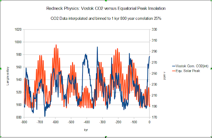
The electric company where I live does not [provide] DC voltage but with a bridge rectifier and a battery I can fix that. Not all that interesting but useful. Using 65N or 60N gives you the equivalent of a stray voltage that can create interesting patterns but with a sphere you would want to use the average applied voltage and peaks to figure out how to design your system.
At the Equator, you have a signal that is rectified with respect to either pole, so instead of a ~20ka cycle you have a doubled 10ka cycle. With that base you can get some neat transients. Add the oceans for a filter and you can get rid of a lot of the transients.
So just on the precessional cycle you can expect multiples of 10ka +/- about 2Ka which would be your strongest frequencies. When you combine that with the other orbital frequencies you get something like this.
Oh, that would be Berger solar and Vostok CO2 both archived at NCDC
captdallas,
nice work. the frequencies align. But the amplitude envelope cycles in and out of 100Ka phase withe VostokCO2.
Joel, “But the amplitude envelope cycles in and out of 100Ka phase withe VostokCO2.”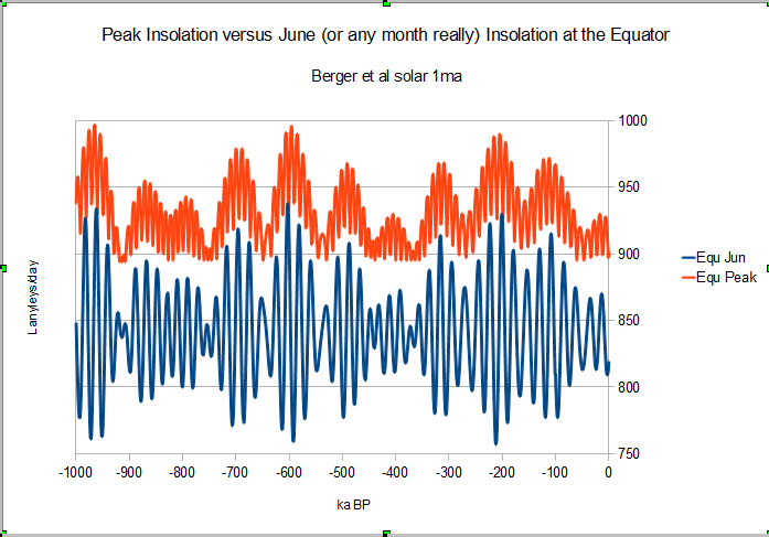
Here is a different look.
With a water world you would be looking for critical energy levels related to water to start an abrupt change. For biological you would be looking for “ideal” ranges and critical levels. CO2 would be related to both, SST and biological “ideal”. Abrupt de-glaciation would trigger a biological “ideal” where the glaciers retreat and in the oceans close to the melt water with that surge of nutrients.
So if you look at the chart above, you have a nice neat rectified envelope but below you have spikes not centered on the envelope peak. These power surges would not be obvious in a nice smoothed “average” insolation for any particular month. “Averages” have limitations.
Correlation does not imply causation. However, lack of correlation does refute a causal link, as in this post. TY for the Roe catch. Read the article yesterday. Obviously not carefully enough.
Good observation. So convenient to talk about 100 k cycles & no one really looks closely at the data. Thus science stumbles along.
Another representation, from
Bintanja, R. and R.S.W. van de Wal. 2011.
Global 3Ma Temperature, Sea Level, and Ice Volume Reconstructions.
IGBP PAGES/World Data Center for Paleoclimatology Data Contribution Series # 2011-119.
NOAA/NCDC Paleoclimatology Program, Boulder CO, USA
Over 3 million years:
http://climate.mr-int.ch/images/graphs/ice_level_3myr.png
Zoom over past 150’000 years
http://climate.mr-int.ch/images/graphs/ice_level_150kyr.png
With the corresponding temperature reconstruction:
http://climate.mr-int.ch/images/graphs/t_reconstruction-150kyr.png
Of course, ice forming or melting has to follow thermal changes, and it takes a long time to transfer so much energy.
When we split hair about tenths of degrees, we forget the thermal changes that are linked to such change of phase (water latent heat of fusion 334 kJ/kg)
At the current rate of melting, it may take 10’000 years for Greenland to have lost all its ice sheet, and 380’000 years for Antarctica. Until then, other cycles will have developed.
Urgency is a relative feeling.
Wondering why they are so interested in Eurasian ice. Eurasia never developed significant ice sheets. Why not use western North American ice, an area which likewise never developed significant ice sheets?
Ice sheets of Eurasia and North America are given. Both had a considerable ice amount.
from Wikipedia:
http://fr.wikipedia.org/wiki/Derni%C3%A8re_p%C3%A9riode_glaciaire#mediaviewer/File:Northern_icesheet-fr.png
There were substantial ice sheets in Eurasia, to include the British, Scandinavian, Alpine, Barents Sea, Siberian & Tibetan, some of which might however be considered montane glacier systems more than sheets. Plus systems as in the Pyrenee, Caucasus & other mountain ranges..
Once you get divergence from the presumed correlation any explanations just become speculation. I thought you guys at least would be cognisant of that after Al Gore and CO2
Willis, I have been at a presentation of Richard Lindzen in Brussels last year, who showed that for melting the ice sheets as happened during the warming towards an interglacial, you need not less than 200 W/m2 extra heat/insolation. The increase of CO2 and its increase in feedback of a few W/m2 seems not of much help in such periods. But where the 200 W/m2 comes from is still unknown. The most probable candidate is changes in cloud cover, but these are minimal during an ice age (minimum humidity) and increase with higher temperatures…
Still a lot of questions in this “Settled Science”…
It is my feeling that you cannot explain the Pleistocene climate shifts without big shifts in insolation values. But if you try to explain it all solely in terms of NH insolation, you will miss by a mile.
I should finish the the thought:
The ice age was _worldwide_ , from the tropics to the poles. Snowpacks on tropical mountains were thousands of feet lower than today. There were lower temperatures _worldwide_. Insolation changes in the NH cannot account for the _worldwide_ aspect ofthe ice age. When the Holocene began, temperatures increased precipitously _worldwide_. Most significantly, in my view, SST increased _worldwide_.
I have yet to see an explanation of the ice age which explains the worldwide increase in insolation at the beginning of the Holocene, which must have been.
Willis, I found your ‘icebox’ series extremely interesting, and I stand back in awe at your data presentation, thanks very much.
Being an ‘averagely evolved pattern spotter’, by your exposition, I would say that your Milankovitch based insolation changes versus paleo temperature plots would appear to suggest (1) that not every insolation swing correlates with a major temperature swing, but (2) pretty well all of the major temperature increase swings are associated with an upward insolation swing. This suggests to me that SOME of the insolation swings trigger the switch from glacial condition to interglacial condition.
Not, I hasten to add an original observation of mine, but one I first noted in John Kerr’s treatise, the Inconvenient Skeptic.
And I also like Fred Berple’s post picking up the 2kA cyclical blips that help with the Minoan, Roman, Medieval and current warm periods.
Imarcus.
Dear Willis,
Look at the wave equation and gain an understanding of oscillations. A pendulum (the ice age cycle) will react to a perturbation depending on where it is in its swing. A warm earth is hard to heat up. A cool earth is hard to cool down. The Milankovich swings depend on the current heat state of the earth when they occur. Milankovitch is an important but not sole factor in the earth’s temperature cycle. CO2 is an insignificant but not sole factor in the temperature cycle…but we already know that. I refer you to John Kerr for an excellent description. Sorry, not peer reviewed….but makes sense to me.
Dear Swifty,
I’m pretty conversant with the wave equation and multistable systems, and agree that the Earth is a highly non-Markovian dynamical system, but do not quite see the mathematical analogy you are trying to establish. Also be aware that the wave equation describes oscillatory propagation of information and energy in space and time. The equation I think you are trying to refer him to is the (harmonic?) oscillator equation, which is not the same thing. In particular the “pendulum” you are trying to describe isn’t being driven by a passive force, and there is no mathematical equivalent of mass or force present. What is happening is nonlinear feedback in an open, bi- to multistable system with multiple knobs — an oscillatory variation in the efficiency of heat trapping by the Earth as it sits in the remarkably stable flow of light energy out from the hot surface of the Sun on its way to eventual thermal equilibrium with the rest of the Universe at its very low absolute temperature. Not really either a wave equation OR a pendulum, although one might make an analogy with a damped, driven pendulum with some work.
rgb
Just for a walk on the wild side, what if we have the causes of precession incorrect?…
http://www.google.com/url?sa=t&rct=j&q=&esrc=s&source=web&cd=1&cad=rja&uact=8&sqi=2&ved=0CB4QFjAA&url=http%3A%2F%2Fwww.binaryresearchinstitute.org%2F&ei=497EVICtE8azoQSM2YKwBQ&usg=AFQjCNHwR2J2j90PGGhyxMYr5twpGQzykw&sig2=eRVmqva7tR3WunDV7E-Imw
Under evidence for…http://www.binaryresearchinstitute.org/bri/research/evidence/lunarcycle.shtml
“Scientists look back in time to before the last ice age using stunning 3D radar maps of Greenland’s ice sheet”
http://svs.gsfc.nasa.gov//vis/a000000/a004200/a004249/4249_Greenland_Radiostratigraphy_MASTER.webmhd.webm
Interesting
http://www.dailymail.co.uk/sciencetech/article-2924272/Scientists-travel-Ice-Age-stunning-3D-radar-maps-Greenland-s-ice-sheet.html
Very nice!
http://svs.gsfc.nasa.gov//vis/a000000/a004200/a004249/4249_Greenland_Radiostratigraphy_MASTER.webmhd.webm
fingers crossed
http://svs.gsfc.nasa.gov/cgi-bin/details.cgi?aid=4249
watch video
What’s interesting about that video is that, apparently, most of the volume of the ice-sheet was laid down during the interglacial period, with considerably less left over from the preceding glacial period. Even some at the bottom left over from the previous interglacial.
More snowfall during this interglacial than during the preceding glacial period?
I did not quite understand this.
Why is there so little ice left over from the last interglacial? We are in an interglacial now, but don’t see massive melting of the ice sheet. Instead we see a massive dome of holocene ice accumulation.
If we went straight into an ice age now, we would see New Ice Age ice ice overlying a thick holocene layer. And presumably it would stay like that until the next interglacial.
Or is the ice at the bottom of the Greenland sheet constantly melting and flowing into the Atlantic?
Ralph
Glacier 18,000 years ago.
http://oi62.tinypic.com/a1pvdj.jpg
http://www.vukcevic.talktalk.net/AT-GMF.gif
As a matter of additional info for those who are not aware. The periodicity of precession is 23K years, the periodicity of obliquity is 41K years and the periodicity of eccentricity is 100K years.
As an additional reminder all representations here are based on limited data sets of temperature proxies.
@Willis:” Is it true that looking at the first difference of the temperature improves the correlation? Yes, it is … but for the wrong reason.”
Which might lead some to conclude that using first difference of temperature is ‘wrong’, betraying a certain amount of confirmation bias (i.e. looking for data which confirms our preconceived notion of how nature must behave).
Instead we should step back and look at the ‘thermometer’ itself (delta-O-18), which is the ratio of the two most common stable isotopes of oxygen in the atmosphere: O16(99.759%) and O18 (0.204%) (with O17 making up the remaining 0.037%). But the ratios are slightly different in terrestrial bodies of water and ice because the lighter isotopes bound to water molecules are more likely evaporate and subsequently precipitate back to the ground or oceans. (O18: freshwater 0.1981%, seawater 0.1995%).
It’s a rather subtle and noisy process, so not a proxy which has a simple linear relationship to temperature like mercury expanding in a tube. It’s easy to fall into the ‘engineering fallacy’, which makes us believe that all thermometers read ‘temperature’ directly from nature. It’s much more complicated than that. So to extract temperature there must be a complex model embedded in there somewhere (which have a tendency to be wrong).
So these isotopes are more sensitive to changes in state, than absolute temperature, which might explain why delta-temp correlates better than absolute T.
Note the findings of Dansgaard in 1964 (the pioneer in paleodating):
Here is something to think about. The temperature curve looks like a capacitor response to a series of charges of different voltages. The rise is rapid but the discharge can take 100k years.
“The rise is rapid but the discharge can take 100k years.”
That’s not a typically charging scenario. Charging is usually slow, discharge much faster relative to charging.
The usual model of electronic circuit which generates the cyclic slow-fast response is called a relaxation oscillator
https://en.wikipedia.org/wiki/Relaxation_oscillator
The circuit must contain at least two components 1) an accumulator (e.g. capacitor) which integrates some increasing quantity (e.g. charge) and 2) a threshold device (e.g. neon lamp etc) which fires or breaks down at some positive threshold, resetting the accumulator back to zero, creating this characteristic pattern, slow rising-fast falling</i?
http://hyperphysics.phy-astr.gsu.edu/hbase/electronic/ietron/unijun5.gif
Relaxation oscillator models fit some natural phenomena very nicely, e.g. earthquakes: strain builds up slowly then released quickly when bedrock fractures.
But the glaciation history, viewed in correct temporal order, shows a different pattern: fast-rising, slow-falling, which doesn't fit this kind of relaxation model:
http://www.brighton73.freeserve.co.uk/gw/paleo/400000yearslarge.gif
So not clear what this 'fast-rise' mechanism is. A time-reversal of discharge seems to be like a time-reversal of an explosion (which violates some laws of thermodynamics).
But a fast-rise of temperature per se doesn’t necessarily violate physics if there is hidden or latent agent causing it.
Just saying.
Perhaps your charge and discharge are inverted. The ‘charge’ is the slow accumulation of ice during the glacial. The ‘discharge’ is the sudden melting of the ice.
I see no reason why you cannot accumulate negative energy (coldness) rather than positive energy (heat). It the same process. You are just springing back to the ‘norm’ (interglacial), from an unnatural state (ice age). You can either compress a spring, or extend it.
R
“Perhaps your charge and discharge are inverted. ”
Yes, I realized the same idea while reading Craig Loehle’s post below,but with the break in the Bering Dam causing the ‘discharge’ and the rebuilding of the dam over several cycles as the ‘charging’.
See http://wattsupwiththat.com/2015/01/24/the-icebox-heats-up/#comment-1843647
Actually in fluids we have this type of response with a flap valve inlet to a reservoir and a small outlet. The reservoir fills quickly when pressure pushes the flap valve open, and drains slowly when the reservoir drains through the small hole. Like dams on rivers, fast fill, slow drain. Many similar devices in hydraulic systems. Or consider a modern electric drill. Half hour charge, several hours of discontinuous use.
What is the inverse of temperature? Maybe we are measuring the wrong parameter.
My take is that the Milankovitch parameters are sometimes a “trigger”, but the major 100kyr event is some type of ocean-current/atmospheric dynamic + ice-sheet dynamics + albedo feedback. A complex, non-linear juxtaposition of effects.
There, solved the problem. 🙂
What about the Earth’s magnetic field?
Is the Earth’s magnetic field reversing now? How do we know?
Measurements have been made of the Earth’s magnetic field more or less continuously since about 1840. Some measurements even go back to the 1500s, for example at Greenwich in London. If we look at the trend in the strength of the magnetic field over this time (for example the so-called ‘dipole moment’ shown in the graph below) we can see a downward trend. Indeed projecting this forward in time would suggest zero dipole moment in about 1500-1600 years time. This is one reason why some people believe the field may be in the early stages of a reversal. We also know from studies of the magnetisation of minerals in ancient clay pots that the Earth’s magnetic field was approximately twice as strong in Roman times as it is now.
http://www.geomag.bgs.ac.uk/images/dipmoment.jpg
http://www.geomag.bgs.ac.uk/education/reversals.html
While the Milankovitch cycles suggest a good place to look for ice ages, we my be making the same mistake the warmers are making – looking in the wrong place. We know there is a some 400 year cycle that we think is linked to sun spots. Could it be the the 100,000 year cycle is also linked to the sun? It’s possible that in warmer times, the sun burns hotter causing waste build up in the core. The cooler time are the result of the waste products mixing with new fuel for another cycle. The time it takes for the heat to reach the surface could also explain the lack of neutrino issue as well because we could still be receiving the heat from the last warm cycle long after the last neutrino peak was reached.
Just a thought reached with far [too] little knowledge of how the sun works.
Last I heard, it take a photon 100,000 years to make its way to the surface. Could a fluid body 860 thousand miles in diameter have a 100 ky cycle? 14C has too short a half-life to tell us. 10Be from ice cores would go back maybe 6 or 7 cycles, but I haven’t come across any yet googling the images. If we find a long Beryllium records (perhaps from sediments) Willis could run his periodicity program and solve the problem.
Currently (and recently) storms have been observed on Saturn and Uranus. It is impossible to say if these storms are out of the ordinary or a result of better or ‘for the first time’ observations. However, it is interesting if we are supposedly seeing an increase in storms here and also on Saturn and Uranus. That is assuming what we have on earth is an increase as opposed to many more people living in harms way. Perhaps the trigger for more storms may not be the peaks or troughs of the suns output but the change? Just thinking.
These are great blogs.
Willis The insolation at 65 N is driven by earths precession and obliquity – there are coincident temperature pekas of relatively small amplitude. The 100000 year temperature peak is obviously related to the eccentricity. You need to include in the plot the changing insolation at the equator or intra tropical region. The climate represents the effect of all three orbital parameters obviously the 100000 year periodicity in the ice ages is mainly eccentricity driven. Where is the mystery?
+1
Dr. Page is makes a good point. The eccentricity is different from the other Milankovitch cycles in that it actually alters global average insolation . That has a much more direct impact on global climate than insolation in a particular area at a particular time of year. So it is hardly surprising that a signal shows up there. There is not just one factor that controls everything.
The only 100 kyr mystery is that the insolation variation due to eccentricity is just 0.45 W/m2, just 12% of doubled CO2. Almost like there might be some sort of amplification.
I thought that obliquity was just an apparent consequence of precession. Obliquity on its own cannot exist, a planet cannot rock forwards and backwards. So counting obliquity and precession is like counting the same thing twice ?
Willis See green curve in Fig4 at
http://climatesense-norpag.blogspot.com/2014/07/climate-forecasting-methods-and-cooling.html
Note approx. 400000 year periodicity which has been identified in the geological record going back 400 million years.
Unable to find any reference to 400kyr power in the link. Strange comparison of Miocene and Hollowscene ™ power spectra that ignores the Pleistocene?
Gymnosperm See FSg 4 look at the pattern on green curve . simplest illustration – see amplitude peaks at 600,000 and 200000. – go on forwards at about 200000 year intervals – Actual intervals vary about some central mean. say 395 – 405 thousand. +/-
Gymno — the point was simply to show that similar periodicities are found in a Miocene section.
The 400000 year periodicity has been seen in the Silurian. The point is that these basic periodicities have been stable and affecting the climate for hundreds of millions of years.
Sorry comment should read go forwards at approximate 400,000 year intervals
I agree completely, Willis. With your observation that you love pain, that is.
I do find it intriguing that somebody would consider the derivative of the temperature to be the important signal when in fact the derivative of the temperature is not the temperature. In essence what one must conclude is that there is a BRIEF INTERVAL where the temperature increases quickly in the 20-30 ky range or periodicity, but that it doesn’t last long enough to actually melt anything, while at 100 ky it warms as about the same rate in spite of having almost no driving at 65 N but the warming lasts long enough to increase the temperature substantially. Say what?
In actual fact, nothing “orbital” is this sharp. We’re talking 1000-2000 year intervals here, and again in actual fact the planet can warm an enormous amount in 1000-2000 years. If ice cores are to be believed, it can warm by 5-6 C in as little as a 100 years, and that is on the SLOW part of the cycle, e.g. the start of the last interglacial. And then there is the Younger Dryas, the Eemian peak, and more.
In the end, the 100 ky “problem” remains, the countervariance of annual insolation and annual temperature problem remains, the “cause of the Little Ice Age” problem remains. None of the explanations are particularly plausible and none of them hold statistical water — the best that can be said for them is that they are possible, except when even that is denied them.
rgb
How about some side effect of magnetic fields being a factor ? Vukcevic’s Polar temperature graph is intriguiging, you (rgb) produced a co2 versus temperature graph with a 67 year harmonic, the Suns corona has a 67 year period, which is surely a result of a magnetic field. Do glaciations tie up with magnetic field excursions / reversal ?
Very unlikely since there isn’t correlation with the Earth’s reversals. Houever there is strong correlation between solar activity and Jupiter/Saturn magnetosphers’ orbital interactions. Since both Earth and sun have regular reversals it is possible that the two gas giants occasionally do have magnetic reversals as well, which may of may not be synchronous with some of Milankovic cycles. If such do last for a milenia or longer the solar magnetic activity would have a very long type of Maunder Minimum, and if so an ice age might follow but in both hemispheres simultaniously. Outer planets magnetic fields have been measured only in recent decades so above is.clearly in the realm of speculation.
Since earth enters ice houses about every 150 million years, a cosmic cause is indicated, as per the galactic arm hypothesis of Shaviv, et al. Once out of a hot house into an ice house, other terrestrial & ET factors determine just how much ice there will be, such as the position of the continents. Major ice sheets didn´t develop during the Mesozoic (Jurassic\Cretaceous) ice house, for instance, as did occur during the two Paleozoic ice houses.
Once in an ice house phase, it is pretty well understood how glaciation happens. Snow that falls in winter doesn´t melt in summer. Over tens of thousands of such summers, you get not just more montane glaciers but vast domed ice sheets. High latitude insolation changes are IMO strongly implicated in starting ice ages in this sense of the term. Milankovitch cycles account for the 40 Ka periodicity at high statistical levels.
Why I see little problem for Milankovitch theory in the longer periods of glaciation in the latter Pleistocene is that the 40 Ka cycles don´t go away. They´re still there & still well explained by insolation. It´s just that they now occur within longer periods of glaciation. They cause the ice sheets to wax & wane. If there´s a problem, it´s in showing what caused the longer cycles within which the shorter ones still operate. IMO obliquity & eccentricity do it, along perhaps, as noted above, with increased albedo due to more ice as the planet cooled during the first half or so of the Pleistocene.
denniswingo
January 24, 2015 at 11:36 pm
“There is another thing that bothers me about these types of analyses. It assumes a perfectly round and perfectly flat Earth. At sea level the instantaneous insolation is about 1000 watts/m2. At 6,000 feet that number is closer to 1175 watts/m2 and at 10,000 feet is closer to about 1250 watts/m2. The northern hemisphere at higher latitudes is at a much higher altitude than the southern hemisphere at the same latitude.”
Willis Eschenbach
January 25, 2015 at 1:17 am
denniswingo January 24, 2015 at 11:36 pm Edit
Willis, I believe the point of denniswingo’s comment is that the topography of the ice sheet is in play (not just the mountains). A three km high ice sheet, like a mountain, is going to still be freezing on top despite the insolation (a large amount of which is also going to be refleccted back. I think a missing factor here is the following: During much of the latter part of glacial period, the relative humidity is very low (which attenuates accumulation) and perhaps a good part of ice reduction is by sublimation with little part played by insolation.
A number of other factors are at play as well. As the ice thins there is a certain amount of crustal rebound partially maintaining altitude of the the top of the ice sheet, increasing humidity, rising sea levels, all without a strong correlation to insolation. Anyone up to calculating how long it would take to reduce the ice thickness, say to half, by sublimation at a realistic temperature profile for the period? After all, Kilimanjaro showed a significant difference in a decade or so.
The following are in your face Milankovitch cycle theory killing deficiencies/failures which unequivocally support the assertion that insolation at 65N does not and cannot physically cause the glacial/interglacial cycle. The theory that insolation at 65N ’causes’ the 100,000 year glacial/interglacial cycle (note the glacial/interglacial cycle was a 41 kyrs period from 2.6 million to 1 million years ago and then suddenly for unexplained reasons to changed to a 100,000 years) is a Zombie theory.
A Zombie theory/mechanism generates piles and piles of anomalies and paradoxes but is still kept alive as the correct solution is not known which makes it impossible to kill the Zombie theory.
Field after field of science have Zombie theories which generate piles and piles of anomalies/paradoxes.
http://en.wikipedia.org/wiki/Milankovitch_cycles
This recent finding that the planet cyclically abruptly cools both poles should have been the final stake in the heart of the Insolation at 65N theory (Do you get that insolation in the summer is maximum in the Southern hemisphere when it is minimum in the Northern hemisphere?), but somehow the insolation at 65N still lives in the imagination of the public and the warmists.
http://earthobservatory.nasa.gov/Newsroom/view.php?id=24476
Don’t forget that because Earth’s orbit is elliptical the orbit speed is increased at perihelion. As eccentricity increases the Earth spends less time close to the Sun not only due to the path of the elliptical orbit but also because it is traveling faster through the orbital path when close to the Sun. More time farther from the Sun, less insolation at the surface. Lower obliquity during a higher elliptical orbit enhances the effect. The only times that Earth has entered an inter-glacial over the last 800k years is when eccentricity is low, obliquity is high and NH summer solstice is at perihelion. Whatever the proxy temps say, whatever the charts depict, whatever the whatever, there is no doubt the inter-glacials happen at certain times when orbital parameters are just right. Whether that is the cause or whether that is causing something else is the question.
Here is my understanding of how this could work. One of the key factors in an ice age is the freeze up of the Bering straits, which then prevents circulation of water into the arctic. This is gradual as water level lowers and ice increases (gradual cooling) but when it gives way it is more sudden and the ice begins to melt rapidly. These processes are threshold events and take a very long lag to get to. They are related to northern hemisphere insolation but also to total ice volume which lowers sea level and makes the straits more of a barrier.
Sandal, C. and D. Nof. 2008. The collapse of the Bering Strait Ice Dam and the Abrupt Temperature Rise in the Beginning of the Holocene. J. Physical Oceanography 38:1979-1991.
Thinking along similar lines, Ewing & Donn, two of the world’s leading oceanographers back in the late 50’s, hypothesized that rising sea levels at the end of the last inter-glacial led to an increase in warmer water flowing into the Arctic Ocean, causing it to become ice-free and providing a rich source of moisture for the atmosphere to draw on. Moist surface winds blowing towards Northern Canada, Europe and Eurasia then bought the snows which enabled the ice sheets to start forming :
http://strongasanoxandnearlyassmart.blogspot.co.uk/2011/07/scientists-predict-another-ice-age-is.html
Maybe the alarmists are actually right, to hyperventilate about the possible loss of Arctic Sea Ice, even if it is for entirely the wrong reasons!
Yes. Noted this also in a comment to previous thread. And YD was almost certainly ice dam related also. The resulting meltwater pulse interrupted North Atlantic thermohaline circulation.
As a gedanken experiment, the Malasian air crash is in 30 meters of water at the center of the strait between Malaysia and Borneo. At the peak of the last glacial about 20 millenia ago sea level was about 120 meters lower. That part of the western Pacific would have been dry land, including the entire Strait of Malacca with maximum depth 37 meters. So ENSO would have been different. Pacific currents would have been different. We know the Gulf Stream at the Florida Strait was significantly weaker at the last glacial maximum. (Nature 402: 644-648 (1999)) It is quite possible that the main climate mode for the past million years is ‘glacial’, but after enough ice mass builds and sea level drops some ocean threshold is crossed that increases poleward heat transport from the tropics causing the fairly sudden (about 10-12 millennia) melt into an interglacial. Henry’s law and Le Chatelliers principle would make CO2 a positive feedback to that per ice cores, with a lag on the order of 800 years. (Gore had it backwards. CO2 lags.) Sea level rise, CO2, albedo, etc, eventually ‘stabilizes’, poleward heat transport ‘renormalizes’ and the process starts over, with growing ice sheet albedo being a significant cooling feedback factor. Just a gedanken.
The Bearing Strait is not the full answer.
The Ice Age ‘breaks’ and ends just when it is reaching its maximums, not when it had already started melting. There is no mechanism I can see that would ‘break’ the Bearing Straits dam, while the Ice Age is still at its peak.
Ralph
William states “Orbital eccentricity’s impact on 65N insolation is the smallest of all the orbital parameters yet for some unexplained reason the glacial/interglacial cycle follows a 100,000 year cycle. Note the glacial period ends when the Northern hemisphere is closest to the sun in summer which occurred 11,000 years ago. The Southern hemisphere is currently closest to the sun during the Southern hemisphere summer (opposite to the orbital position 11,000 years ago) which is the position to terminate interglacial periods.”
Link below for this interesting walk on the wild side…”In examining the phenomenon of the precession of the equinox (which was the original impetus for the development of lunisolar precession theory) we have found that a moving solar system model is a simpler way to reproduce the same observable without any of the problems associated with current precession theory. Indeed, elliptical orbit equations have been found to be a better predictor of precession rates than Newcomb’s formula, showing far greater accuracy over the last hundred years. Moreover, a moving solar system model appears to solve a number of solar system formation theory problems including the sun’s lack of angular momentum”….
http://www.binaryresearchinstitute.org/bri/research/evidence/lunarcycle.shtml
…”Under the current lunisolar theory of precession it is assumed that the earth goes around the sun 359 degree 59 minutes and 10 arc seconds in a Tropical year, the period from like equinox to like equinox, which is equal to 365.2422 rotations of the earth. This is true if you measure the position of the equinox relative to the fixed stars “OUTSIDE” the solar system but it is not true if you measure the movement of the equinox relative to the sun or moon or other objects “WITHIN” the solar system, where the lunar data shows us that the earth goes around the sun a complete 360 degrees in a tropical year. Unfortunately, neither NASA VLBI nor any other official agency measures the earth’s orientation relative to nearby objects, so the paradox goes unnoticed”…
Does nothing to explain why the cycles we measure, but certainly would relate to why we find no correlation in the climate record.
Of course, the Earth’s climate has been following cycles of cooling and warming, throughout it’s history. Now we are living in the holocene era, a period of gradual warming of the climate, following the ice age, which has ended over ten thousand years ago. Some are saying that the climate is changing in a more rapid manner startig with the 20th century, mainly because of human influence. The greenhouse emissions are the most pointed cause of climate change, especially global warming. Some other theories exist, however, which point to the oceans, which are considered to be the main influence on global climate. The two world wars of the past century, especially the naval battles are thought to have had an important role in changing the climate. Have a look at http://www.warchangesclimate.com/ for more info on the matter.
Has anyone tried to correlate temperature variations (or some portion thereof) with the impact of episodic glacial meltwater releases? I know there is research concerning the AMOC as well as the Bering Strait and how they influence (and are influenced by) global climate and freshwater discharges. It would seem plausible that freshwater pulses (and the specific timing of major releases) could interact with both oceanic currents and high latitude insolation to mask any single influence’s precise impact. Major freshwater releases have abrupt tipping points (dependent upon local topography) that would not necessarily coincide with orbital cycles. For example, if freshwater pulses changed in frequency, volume or both, perhaps there is a non-orbital mechanism for shifting between 41k year and 100k year cycles?
In any numerical analysis, before even getting into the numbers, I always want to know how accurate the numbers themselves are and what assumptions went into generation of the numbers. So before beginning an analysis of cyclicity of past glaciations, I’d like to know the basis for data making up ‘geological temperature swings’ and what assumptions went into generation of those numbers. In a response to Willis’s earlier post, I pointed out some of the problems with these numbers. In a nutshell, we can date the last two glaciations (back to a few hundred thousand years) with various istopes (14C, 10Be, 37Cl, U series, and others) but the older glaciations are not directly dated. Since the direct dates we have are from glacial moraines, we know when they occurred, but don’t have temperature measurements. For those, we have to rely on ice cores and deep sea cores, but the problem here is they are not directly dated and their ages are inferential with lots of built in assumptions.
In addition to the dating problems, what assumptions are built into the numbers? In a word, a lot (see my response to the previous post). That doesn’t mean the numbers are wrong, but it does mean that if the assumptions aren’t valid, neither are the numbers. What I’m trying to point out here, is that Willis’s analysis, is as usual, elegant, but the sources of the numbers for ‘geological temperature swings’ are really not very robust for the older glaciations.
Aside from the statistical analyses, there are very serious problems with the Milankovitch theory. For example, (1) as John Mercer pointed out decades ago, the synchroniety of glaciations in both hemispheres is ‘’a fly in the Milakovitch soup,’ (2) glaciations typically end very abruptly, not slowly, (3) the Dansgaard-Oeschger events are so abrupt that they could not possibility be caused by Milankovitch changes (this is why the YD is so significant), and (4) since the magnitude of the Younger Dryas changes were from full non-glacial to full glacial temperatures for 1000+ years and back to full non-glacial temperatures (20+ degrees in a century), it is clear that something other than Milankovitch cycles can cause full Pleistocene glaciations. Until we more clearly understand abrupt climate changes that are simultaneous in both hemispheres we will not understand the cause of glaciations and climate changes.
I have to agree 100% with this. My geology degree is long in the past, but I enjoy reading articles and books regarding the Ice Ages and the standout feature, without a doubt, is the extreme and rapid climate instability during the Ice Ages. Dansgaard-Oeschger and Heinrich events occur in the blink of an eye in geological terms and in the case of the YD we are talking a decade or two. These types of changes are far beyond anything witnessed by anyone today. In retrospect the Holocene is a time of extreme climate stability compared to the previous 100,000 years. And that is a very sobering thought.
My viewpoint as well. The temperature spikes, known as interstadials, throughout the Pleistocene have been sudden. The D-O spike was the same. The YD stepdown was typical, though we have much better resolution on these nearer events than the older, less well resolved events as recorded in the ice cores.
It should be said that Don Easterbook is a professor emeritus in glaciology.
Yes, I know that Don is Dr. Easterbrook, PhD Geology, which is why I enjoy his commentary and articles.
As an aside a memorable moment for me was when our resident palynology expert, the late Dr. Bill Matthews of UBC, took us students to an area near the mouth of the Fraser River to take a core of the peat bog. The core was around 5 meters (15′) in length and consisted, as expected of peat which abruptly ended in sand which marked the start of Ice Age deposits. For a geology student this abrupt change was unforgettable, plus the fact that Bill Matthews told us that the lower layers contained Oak pollen which indicated a warmer and drier climate in the early Holocene. Seeing all that in a peat core was amazing.
E. J. Mohr:
No question, the Holocene started quite abruptly and ice core data shows this clearly. Other proxies do as well, as in your example.
It’s as if someone ( who?) threw a switch.
Here allow to demonstrate…[click]…
See?
>>oak pollens
The oak pollens at that latitude demonstrate that this was a much warmer climate, at a time when the ice sheets were still present (but melting).
The M. Cycles cannot explain this, because the M.C.-induced insolation levels are up and down all over the place – while the ice sheets are doing something completely different and completely disconnected to the changes in insolation. The Ice Age is often still busy growing ice sheets, while insolation is at its absolute peak.
.
The answer to the 100,000 year Ice Age conundrum has to lie in something like a radical change in cloud cover – something that can protect the surface from increasing M. Cycle insolation, and keep the summers cool. All you need is a string of summers with temperatures below that required to melt all of last winter’s snow, and you have just begun the process of a new Ice Age. And this will continue, for as long as the excessive cloud cover persists.
However, when you reach the point at which the clouds part and disappear (for some reason), then you can indeed have really baking hot summer temperatures, with majestic oaks growing next door to some huge (but rapidly retreating) ice sheets.
R
The real paradox is albedo. Just when glaciers reach their maximum extent, and albedo reaches its highest, everything starts to melt. Makes one wonder how much albedo really counts.
Palynology is wonderful stuff and I wonder why you don’t see any climate reconstructions based on such studies.
An infallible way to second varves, tree rings, etc. or so it seems.
Methinks the switch may have had an embedded link, but she no work for me. Meanwhile where I sit in SE BC I can look out the window and see the Holocene Neo-Glacial ice on the mountains. I can see all the moraines that indicate the LIA and possible earlier ice advances. The mountains tell a very interesting story, but that is not all.
The palynology and midge data from the lakes tells us that the Interior Wet belt forest that exists here may only be around 2500 years old. Prior to 4000 years ago the forest type was different – mostly spruce and pine which indicates a warmer drier climate. In southern BC the lake sediments in the upper Ashnola River speak of much warmer climate with frequent forest fires. So, the idea of static climate is a very bad idea, as the evidence does not support it. Getting back to the Ice Ages I certainly agree that the changes are so sudden that is indeed as if a switch was turned on or off. And that is where the problem starts.
Hi E.J Mohr
“So, the idea of static climate is a very bad idea, as the evidence does not support it. Getting back to the Ice Ages I certainly agree that the changes are so sudden that is indeed as if a switch was turned on or off. And that is where the problem starts.”
——————-
There is an explanation for that fast switch turn.
Is only an illusion created by the certainty given to the length of the Ice Age, the 100K years long.
You see in a scenario of a much shorter length that will not be the case.
You can not say the same thing if glacial periods only 5K years long.
It seems fast and quick only because of the long length of the glacial periods, which very well could be a very wrong estimation.
Basically it is estimated that way because the ice core data temp record is considered and interpreted as a true representation of the global climate temp variation. The temp signal in the ice core data is considered as the true signal of climate.
That is what happens when M. Cycles theory “marries” the ice core data……. they prove each other and as a result we get a wrong picture (borne) of climate and climate change and we end up considering the polar regions variations and temp records as a true representation of climate change, wrongfully.
You see if we were to estimate the climate and the GW for this last century by relying in the polar Arctic temp records, we be already in a very quick strong and a runaway GW.
The arctic did warm much more than what was projected even from the Runaway Global Warming theorists.
In same time the climatic global picture was different.
Relying in Arctic temps shows that we already must be in a AGW.
That is the distortion of Polar regions records and data while recording the climatic impulse, in too far and a too wide error.
The latest adjustment of Y.D is simply because even it is too exaggerated due to the distortion effect of the ice core data.
cheers
whiten – I was speaking of lake sediment data in British Columbia during the Holocene where already we see that climate is not static, and all this during the benign Holocene. As far as orbitally tuned data, well Don Easterbrook has already explained that the method of tuning using M-cycles will skew the results so that you cannot help but find the M-cycles. OTOH as TTY pointed out on another thread there is no really good way to date sea bottom cores, and kilometres of ice, where the annual layers are impossible to discern. Until a better solution is found, if ever, we have to go with this, bearing in mind that it may be wrong.
But all is not lost since there are terminal moraines at the southern extant of the NA ice lobes that have been dated and they match with the 100 ky cycles. There is also the famous Devils Hole Cave and other caves that provide independent, and non tuned data. The end result is that, although science is not settled, I think we can safely assume for now that the last Ice Ages have been on a 100,000 year cycle with brief interstadials like now. The mystery is still – how and why do Ice Ages end, and how do they start? M-Cycles don’t seem to provide enough solar variation for either process.
E.J. Mohr
January 25, 2015 at 10:30 pm
“The end result is that, although science is not settled, I think we can safely assume for now that the last Ice Ages have been on a 100,000 year cycle with brief interstadials like now. The mystery is still – how and why do Ice Ages end, and how do they start? M-Cycles don’t seem to provide enough solar variation for either process.”
———————–
Hello Mohr.
Thank you for your reply
Let me explain my point again in regard to your statement above.
First, please do understand that I am very aware and clear about the possibility of my arguments to be completely wrong…but this said, I would like to explain a bit further my point.
The length of the glacial periods (Ice Age) as far as I can tell is estimated as 100K years long in accordance of the temp records of the ice cores.
So the ice core data is considered as a true representation of the climatic change because of the polar regions do drive the climate through a cooling period (causing the cooling period) due to the ice build up in the polar regions because of the M. Cycles effect.
So the ice building up in the polar regions causes the the climatic cooling ( Ice Age) as explained through the M. Cycles theory.
So when you say M. Cycles don’t seem to provide enough solar variation for either process…. you lose the 100.000 year glacial period,….. the ice core data at that point is not anymore a correct representation for the length of the Ice Age.
So the length estimation of the glacial periods is at 100K years long only while the ice core data in “marriage” with the M. Cycles effect as a cause, otherwise that estimation becomes completely arbitrary and bears no mark of certainty, but in contrary becomes very dubious and confusing.
The only way to explain the discrepancies between the ice core data and the M. Cycles effect are two possibilities:
1- The M. cycles effect simply good enough (or strong enough) only to trigger the glacial periods and “drive” the glaciation to a point and then fail to drive climate change any further.
2- The M. Cycle effect not good at all to cause or trigger any climate change, but strong enough to drive the extremity behavior of the polar regions during given climate states.
This will mean that the ice core data still represents a climatic signal in the temp records but very much distorted.
In both these cases a new glacial length estimation required, as the current estimated one will be in a very high possibility to be wrong..
Please understand my point.
There is not a fair and a correct ( considered as possibly true) estimation of a glacial period at 100K years long if M. Cycles theory debunked or not considered as the explanation for the Ice Age(s).
There is no any glacial cycles or Ice Age cycles or Interglacial cycles.
All these are periods. If there is any cycles it will be climate cycles which will be made up of glacial periods and Interglacial periods.
And a climatic cycle with a 15 K years Interglacial and a 100K years Ice Age is a very much distorted cycle.
Thanks again for your reply, …….just furthering a bit more my argument…..very possible that I could be wrong…
cheers
whiten – if I understand you correctly you are uncertain as to whether or not Ice Ages actually last 100 kilo years vs interstadials which average a mere 10,000 years. You have correctly deduced that orbital tuning may make the data look like this when, in fact, it could be very different.
As far as I know the southern margins of the continental ice sheets in North America have been dated via non orbitally tuned techniques, using the actual terminal moraines as far as I know, and these tell us that the last two ice advances that were about 100 kilo years apart. So, even without ice cores or ocean sediments we have an independent age calculation. There are also speleothems that give non orbitally tuned data, so again we have reason to believe that the 100 kilo year signal is real. I hope that helps.
E.J. Mohr
January 26, 2015 at 9:24 pm
Yo say:
“whiten – if I understand you correctly you are uncertain as to whether or not Ice Ages actually last 100 kilo years vs interstadials which average a mere 10,000 years. You have correctly deduced that orbital tuning may make the data look like this when, in fact, it could be very different.
————-
Hello Again Mohr.
Thanks again for your reply.
Hopefully you be reading this.
Now , as per above selected part from your last reply to me, I want you to know that I am very certain of the high probability of the possibility that the 100K length of a glacial period is a wrong estimation.
Whether I am wrong or not with that is entirely another matter, but to be honest I have no doubt of it’s fallacy, as the things stand.
Now going further with the rest of your reply.
You say:
“As far as I know the southern margins of the continental ice sheets in North America have been dated via non orbitally tuned techniques, using the actual terminal moraines as far as I know, and these tell us that the last two ice advances that were about 100 kilo years apart. So, even without ice cores or ocean sediments we have an independent age calculation. There are also speleothems that give non orbitally tuned data, so again we have reason to believe that the 100 kilo year signal is real. I hope that helps.”
————
Keeping with as far as you know and with as far as I know, and not trying to doubt and argue the accuracy and the precision of the method in question, as per above, but only taking it in the face value that is of the most higher probable precision and accuracy, even then there still seems to be a big problem with it as a proper correct valid and indisputable evidence for the 100K years length of the glacial periods.
The first problem is that it can be clearly shown that is not even better than the ice core data, while it is considered as a kind of proof or evidence of the length of the glacial periods, in the very way you are suggesting.
Even with total rejection of the M. Cycles theory, still ice core data shows clearly that for the last 400K years there has been 4 significant ice advances with a frequency of been apart in the ranges from 80K years to 100k years.
I don’t know of any one including me who argues that.
Now coming back to the other evidence that you offer as per above.
When said that “the last two ice advances that were about 100 kilo years apart”, ……actually trying to use the numbers correctly, that will be only considered as ~100kilo years apart, which while considering a 100K years possible length for a glacial period will be more properly represented as a range of 80K to 120K
years apart, and that at a very high precision of the method and measurement.
At that point is simply “saying” and confirming whatever the better record of the ice cores is already” saying”
So while ice core data move from the position of a “conclusive” evidence to a “circumstantial” evidence once the M. Cycles effect not considered as a cause of glacial periods, still ice core data is even better than the one you try to offer as a valid explanation for the glacial length, in the way you do.
So the evidence you offer is only another kind of a circumstantial one and weaker too.
In another way, for the clarity of the argument, if ice core data without the support from the M. Cycles effect move from a 90% probability to 50% PROBABILITY of accurately estimating the 100K years length of the glacial periods, then the other method you offering above fairs much worse, somewhere at 30% probability.
Also, a simple conclusion as put above from you;
“and these tell us that the last two ice advances that were about 100 kilo years apart. So, even without ice cores or ocean sediments we have an independent age calculation”
—
means that the total independence of the age calculation (as per above) from other evidence, like from the ice core data, can only give you an estimation of the length of a glacial period as from ~50k years to ~100K range, with a huge error margin, in any possible definitions of the meaning for “ice advance”.
Further more, for the “evidence ” you offer above to be of any significant meaning and considered as possible to estimate the length of the glacial periods at a 80K years to 100K years range, in its own alone it needs two main Ingredients:
1-The very high precision of the method and measurement used.
2-The very high precision of the climate cycles to be considered.
So even while considering the method and the measurement as of a very high precision, still we need to have the climate cooperate and be to an accuracy of its cycles with the precision of a Swiss clock, meaning that the repetition of the ice advance will be at the precise pattern for any glacial period at any given moment, otherwise the estimated range will be too wide and wider for a wider glacial period.
With a 15k years Interglacial followed by a 100K year supposed glacial period the climate supposed cycles will be anything but not precise, too far distorted, far removed from the possibility of a very high precision cyclic repetition.
Using only ice core data as the data stands, without any further interpretation nearly the same could be claimed, as you claim in your reply to me.
While in the case of ice core data one can cherry pick and show advances of ice every 80K ,100K or 120K year apart, or showing two significant ice advances in the same glacial period at about 80K years apart…..in the case of what you offer the thing is so lose lose that whatever done no one can be blamed of any cherry picking as there no any clear reference.
So in the end of the day, in my opinion, the ice core data is much better than one you offer but still not good enough when M.cycles theory not considered and rejected. That’s how lose lose the evidence you offer is, especially when trying to stand in it’s own “feet” as of some meaning.
Please do forgive me if in the end of the day this argument of mine ends up to be just a result of a figment of my imagination, but only speaking up my mind here, in hope I learn something new.
Thanks again for your reply.
If you read this please offer some feedback to me by replying, if you would not mind…..
Appreciated
cheers
whiten – I suggest you look at the Devils Hole Data which independently corroborates the ice core and deep sea drilling data. Based on that I can say that the length of the Ice Ages is not in doubt, and we can be very confident about that. I would ballpark it as 90% certain or better. There is some wiggle room, but there is very little doubt that the last million years have been mostly cold. The Devils Hole project is here:
http://pubs.usgs.gov/fs/2012/3021/pdf/fs2012-3021.pdf
Now if you accept the data, and I do, then the problem really comes down to how this whole business of Ice Ages and Interstadials comes about.
E.J. Mohr
January 27, 2015 at 1:08 pm.
Thanks.
Your reply very appreciated.
Very helpful link there.
While the paper goes to a fair length of explain the probable fallacy of Milankovitch theory still I can’t find any thing that it can really support in it’s own in regard of the length of the glacial periods.
The main contribution of Devils Hole Research to the paleoclimatology is the debunking of the Milankovitch cycles, which you know I am not arguing.
Also its further contribution consist mainly about the interglacials and still there nothing much about glacial periods.
Let me brink some copy paste as to explore this in more detail:
From the paper The Devils Hole oxygen-18 :
—-
1-“The Devils Hole oxygen-18 time series is
primarily a proxy indicator of paleotemperatures. Unlike oxygen isotopes in deep-sea cores, it is not a record of past global ice accumulation in terrestrial systems. Rather, the time series
appears to correspond, both in timing and relative magnitude,to variations in paleo-sea-surface temperature…….etc. ” (self explanatory)
2-“The Devils Hole record is also highly correlated with major variations in paleotemperatures recorded in the Vostok ice core from the East Antarctic Plateau”
And the third one below is the only time when glacial periods may have being mentioned while in the point of trying to debunk the M.hypothesis :
3- “The high correlation between the Devils Hole record and the ice core record at Vostok on the East
Antarctic Plateau indicates a consistent interhemispheric timing of Pleistocene ice ages, which also is not consistent with the Milankovitch hypothesis.”
——-
So either I am missing something or the paper is not saying much at all about the length of the glacial periods.
Then according to the copy-paste number 2 and 3 the high correlation claimed with Vostok is simply of a supportive nature to that ice core data in the estimated timing of the glacial periods and also to a degree it gets back some support from that ice core data for its own validity and accuracy as a proxy indicator of paleotemperatures.
Again the ice core data is a much stronger evidence than the one mentioned. The paleoclimate data is heavy effected by the ice core data more than FROM any thing else, as far as I can tell.
Besides there is a probable logical fallacy in the way that you may read and interpret the above when considering the “high correlation”.
So to speak the ice core data are considered beyond any doubt as “polluted” or “distorted” to a degree by M.Cycles effect.
They get “polished” before considered as paleoclimate data or accurate paleotemperatures,.
You see the real temp ice cores record swings between the glacials and interglacials are at about
8C to 12C, but it is adjusted to half of that when considered in what it means in real climatic terms, somewhere at about 4.5C to 6C.
So trying to squeeze from that paper more than it actually says and claims it creates the problem of much higher supposed correlation where M. Cycles do somehow end up to have a “polluting” and distorting effect in that Devils Hole temp proxy record too..:-)
I accept that record for what it seems to me to be, probably very much so that we may diverge at that point.
In the end I can’t rate it as more than another weak circumstantial evidence still inferior to the ice core data.
But that is me at this point, probably wrong.
Thanks again for the link.
First time I read that paper, thanks to you. Pleasant.
cheers
Astley:“A Zombie theory/mechanism generates piles and piles of anomalies and paradoxes but is still kept alive as the correct solution is not known which makes it impossible to kill the Zombie theory.”
The solution to Zombie theories is sometimes as simple as finding a better reference frame to interpret data which has been correctly collected, but just misinterpreted. A classic example is the apparent ‘motion’ of stars and planets in the sky. The Zombie theories from ancient times tended to invent complicated ‘supernatural’ events and entities to explain the celestial movements. But even in more recent history, Ptolemy’s Epicycles were based on correct observations, but he just used the wrong reference frame.
Imagine trying to reconstruct the path of a vehicle from analysis of the scenery viewed through a window in the vehicle, rather than using a reference point outside the vehicle fixed with the scenery.
Or consider the medical imaging problem (petscan, ctscan etc) where we are trying to infer the shape and extent of some hidden object by viewing the received intensities of a constant but orbiting beam of radiation through different parts of a fixed object. The intensities recorded by the orbiting sensor may seem to have a complicated ‘epicycle-like’ patterns, like this:
http://homepages.inf.ed.ac.uk/rbf/CVonline/LOCAL_COPIES/AV0405/HAYDEN/boxsino.png
from which the original object (2D box) can be reconstructed by the Radon transform, like this:
http://homepages.inf.ed.ac.uk/rbf/CVonline/LOCAL_COPIES/AV0405/HAYDEN/box.png
http://homepages.inf.ed.ac.uk/rbf/CVonline/LOCAL_COPIES/AV0405/HAYDEN/Slice_Reconstruction.html
In meteorology, we use NWP (numerical weather processing) to explain or predict weather events and entities, based on the laws of physics (mechanics, thermodynamics, electromagnetism etc), by decomposing the world mathematically onto 2D, 3D, or 4D grids down to a scale of resolution where individual air parcels can be modeled.
So, do we want to observe these air parcels from a fixed point on the planet model (so we can see how each parcel affects that fixed point)? Or do we want to watch from a reference frame traveling with the parcel (so we can see what’s happening to the parcel itself)?
The answer is ‘yes’. In meteorology (and fluid dynamics in general) we want to be able to use both kinds of reference frame:
1) “Eurlerian”: from a fixed reference, if we want to see how weather changes in a specific location
2) “Langrangian”: from a frame traveling with some ‘material’ entity (storm, front, isoentropic surface etc)
In calculus of fluid dynamics we use the material derivative to analyze weather from both reference frames
https://en.wikipedia.org/wiki/Material_derivative
So, going back to Willis’ post, I’m getting the feeling that we’re correctly (more or less) observing temperature patterns in a time series from a fixed location (65N). But we are seeing some interesting but complicated ‘epicycles’ in the data, which cannot be adequately explained, even using the Milankovich theory. I suspect there is another, more mobile, frame of reference which will unify/simply these Milankovich ‘epicycles’ into some simpler “palm-to-face” explanation.
Thanks, Willis. Very good article showing us facing a too complicated matter.
Willis:
Isn’t the data set actually spliced together from different methods? If the phase is off in the -100kYr to -400kYr range, could that not be a systematic error in one of the methods used to date the implied temperature? That is what I suspect when I see phase errors in anything.
Well, the R^2 of the two is a mere 0.05 … that is to say, the June insolation at 65°N only explains about 5% of the variations in the first difference in temperature. Color me unimpressed.
Imagine an agricultural treatment that correlate with crop yield across a large range of soil and microclimate types, with a R^2 that large.
Or a treatment with that size effect on tire life, or human life.
What look like tiny effects on the R^2 scale can be important when applied at a large scale. With nonlinear dynamics and chaotic systems, small effects can be way more important than you would naively think.
As to your analysis of first differences: it is hardy surprising that derivatives of sines have the same power spectrum as the sines themselves; similarly for derivatives of cosines; with inequalities between the corresponding spectra due to approximation errors.
It might be interesting to you, since you have a lot of the code already written, to regress the first differences on the raw values, then regress the second differences on the first differences and raw values, and see if you can estimate a second-order differential equation whose output approximately matches the raw data streams. Of course you know already from the R^2 value that the match of model to data is unlikely to appear strong.
The “cycle” with a 1ky period seems to be prominent in the most recent 11.5 ky.
Thanks again for your work.
I note there is a tiny bump in insolation @100K years. Can this method find a latitude on Earth where this bump is enlarged?
================
It’s Always Sunny in Philadelphia. I was once a growing bump there.
Like for instance, the Equator?
H/t Capt. Dallas.
============
Nope. No 100 Kyr cycles at the equator either.
w.
Thanks.
======
Nope. No 100 Kyr cycles at the equator either.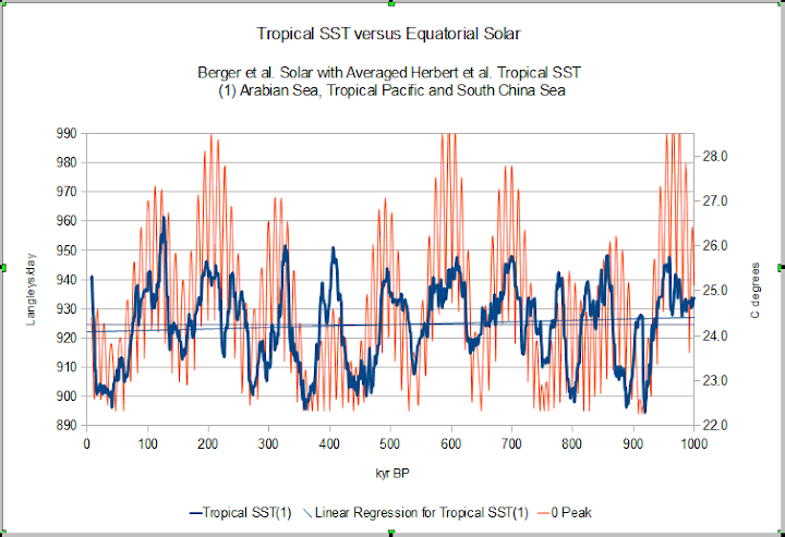
Yes and no. What you have at the equator is ~10ka peaks related to the precessional cycle that vary by about +/- 2ka. That can produce any multiple of 10ka +/- 2 ka. Precessional cycle is the big dog. Eccentricity would be a nudge. Instead of focusing on ice which is remarkably unstable, distorts the Earth’s crust, I focus on the tropical oceans. In fact, Herbert et al. 2010 has Arabian Sea, South China Sea and Tropical Pacific reconstructions that you can bin and average for a fair, tropical ocean reconstruction. The Atlantic reconstruction has some wicked gaps. That and the Berger solar for Equatorial peak insolation, match nearly perfectly for a million years.
The next strongest signal looks like 400kyr, but there is a weak ~100kyr in the mix.
captdallas2 0.8 +/- 0.2 January 25, 2015 at 3:43 pm Edit
I don’t find that at all. Here’s what I get:
I doubt yours, because nobody I’ve read thinks there is a 10 kyr cycle in the insolation data …
But I could be wrong. I just checked my figures, however, and I don’t see any error.
w.
Wilis, PEAK insolation. It is peak that can start melt, that reduces albedo that continues melt if you are looking at ice sheets. It is also Peak that would produce a maximum SST, (the rectifier and battery analogy). I just used latitude (maximum) instead of latitude June. With Eccentricity change you have more days summer or winter plus a little more insolation, so your peak month can slip around a little from what I have read.
Willis, They look like this,
>>Captdallas
Can you make your graphs go the right way….
The trouble with this graph, is that insolation continues to peak, while the ice sheets are growing once more. That sounds counter-intuitive, and in need of further refinement and explanation.
R
ralfellis,
“The trouble with this graph, is that insolation continues to peak, while the ice sheets are growing once more. That sounds counter-intuitive, and in need of further refinement and explanation.”
That is pretty much how it works. The tropical oceans have a convective triggering temperature at around 27.5 to 28.5 C, then cloud cover and deep convection increases allowing more moisture to be transported to the poles to build the ice sheets. Clean ice sheets can survive pretty high insolation so they tend to grow more during higher solar insolation when they are likely to get regular clean snow accumulation. You do have critical insolation depending on how high the ice sheets are, where even clean snow can start to melt. Once you have some melt, the albedo drops and there is increased melt. So you have melt triggering energy and convective triggering temperatures providing two control points.
Ice sheets though are pretty finicky when they decide to collapse, so the orbital cycle doesn’t correlate as well with ice as it does with Tropical SST. So the chart with the Herbert et al. tropical SST versus orbital is the one I prefer to show.
It could have easily been more snow at 65N as less insolation.
=======================
Maslin and Ridgewell 2003 have an interesting take on the eccentricity problem:
http://sp.lyellcollection.org/content/247/1/19.short
Thanks for the reminder. I corresponded with Maslin when researching an Ice Age novel.
I have a couple of comments relative to the data underlying this thread.
First, the peak in both temperature and insolation at 2kyr is not an artifact of the sampling period except for the issue of aliasing which I question in my second point below. The Nyquist frequency at delta-t of 1 kyr is one period per 2 kyr, so the signal at 2 kyr, assuming no aliasing, resolves just fine; however the periodogram value at the Nyquist rate is utterly dependent on sampling phase, and so the amplitude should have very large error bars associated with it. Back when I was doing seismic processing for oil exploration we generally thought a sampled signal should have at least 5 sample points per cycle, rather than the two available at the Nyquist rate. So that portion of data below 5kyr cycle isn’t worth much.
Second, the isotope data are not “point” values, but rather have a sampling window, dependent on field sampling and laboratory methods, which smears time resolution. What is the nature of the sampling window? Can anyone answer this question without my having to dig through discussion of field technique that may not exist anywhere? Perhaps at the top of some column (ice or ocean sediment) the window is minus 500 years to plus 500 years, but column compaction, which occurs in both ice and sediments, might make the sampling window much wider at 100Kyr or 400kyr. On the other hand a very narrow sampling window may leave the isotope data aliased–i.e. placing short period features in the geological column as artifacts in the periodogram at periods of 2kyr and longer.
Finally, I question the value of correlating insolation against temperature, when the insolation may not impact temperature directly, but has to operate through feedback subject to the complex dynamics of the atmosphere, and so forth. Lack of correlation I don’t see as a definitive test of Milankovitch cycles.
From Don Easterbrook – Aside from the statistical analyses, there are very serious problems with the Milankovitch theory. For example, (1) as John Mercer pointed out decades ago, the synchroniety of glaciations in both hemispheres is ‘’a fly in the Milakovitch soup,’ (2) glaciations typically end very abruptly, not slowly, (3) the Dansgaard-Oeschger events are so abrupt that they could not possibility be caused by Milankovitch changes (this is why the YD is so significant), and (4) since the magnitude of the Younger Dryas changes were from full non-glacial to full glacial temperatures for 1000+ years and back to full non-glacial temperatures (20+ degrees in a century), it is clear that something other than Milankovitch cycles can cause full Pleistocene glaciations. Until we more clearly understand abrupt climate changes that are simultaneous in both hemispheres we will not understand the cause of glaciations and climate changes.
My reply
All the above which is what the data shows lends support to my thoughts that solar variability and the primary and secondary effects associated with this solar variability are a big player in glacial/inter-glacial cycles when taken into consideration with these factors which are , land/ocean arrangements , mean land elevation ,mean magnetic field strength of the earth(magnetic excursions), the mean state of the climate (average global temp), the initial state of the earth’s climate(how close to interglacial-glacial threshold it is) the state of random terrestrial(violent volcanic eruption) /extra terrestrial events (super-nova in vicinity of earth or a random impact) along with Milankovitch Cycles. These factors setting the back ground for a general climatic trend for the earth to move in if solar variability did not exist at all.
What I think happens is those factors keep the climate of the earth moving in a general trend toward either cooling or warming on a very loose cyclic or semi cyclic beat but get consistently interrupted by solar variability and the associated primary and secondary effects with this solar variability which brings about at times counter trends in the climate of the earth within the overall trend , or at other times when all the factors I have mentioned setting the back ground for the climate trend for cooling or warming along with what solar variability has been doing in conjunction with these factors , then drive the climate of the earth gradually into a cooler/warmer trend UNTIL it is near that inter- glacial/glacial threshold or climate intersection that makes any further solar variability no matter how slight at that point to be enough to cascade the climate into an abrupt climatic change. The back ground for the abrupt climatic change being in the making all along but when the threshold glacial/inter-glacial intersection for the climate is reached that is NOT ONLY when the abrupt climatic changes occur but the constant swings in the climate from glacial to inter-glacial over short periods of time can take place .
The climatic back ground factors along with the general trend in solar activity driving the climate gradually toward the climate intersection or threshold of glacial versus interglacial, then once there at the intersection the climate gets wild and abrupt.
The climate is chaotic, random and non linear but in addition is never in the same mean state or initial state which makes given forcing to the climatic system not resulting in a given outcome which is why I think there is a semi cyclic nature to the climate but it is consistently being disrupted with counter- trends at times or abrupt changes at times.
If what I say is not on the correct path then why is it whenever the climate strays from its mean in either a negative or positive direction it is ALWAYS brought back to its mean. Why does the climate never go in the same direction once it heads in that direction?
Why is it that when the ice sheets expand the lower albedo /lower temperature more ice expansion positive feedback does not keep going once it is set into motion? What causes it not only to stop but reverse?
Vice Versa why is it when the Paleocene – Eocene Thermal Maximum came about that the increase CO2/higher temperature positive feedback not only did not keep proceeding but reversed?
I will have a follow up post to this one.
My follow up.
Below I list my low average solar parameters criteria which I think will result in secondary effects being exerted upon the climatic system.
My biggest hurdle I think is not if these low average solar parameters would exert an influence upon the climate but rather will they be reached and if reached for how long a period of time?
I think each of the items I list both primary and secondary effects due to solar variability if reached are more then enough to bring the global temperatures down by at least .5c in the coming years.
Even a .15 % decrease from just solar irradiance alone is going to bring the avg. global temperature down by .2c or so all other things being equal. That is 40% of the .5c drop I think can be attained. Never mind the contribution from everything else that is mentioned.
What I am going to do is look into research on sun like stars to try to get some sort of a gage as to how much possible variation might be inherent with the total solar irradiance of the sun. That said we know EUV light varies by much greater amounts and within the spectrum of total solar irradiance some of it is in anti phase which mask total variability within the spectrum. It makes the total irradiance variation seem less then it is.
I also think the .1% variation that is so acceptable for TSI is on flimsy ground in that measurements for this item are not consistent and the history of measuring this item with instrumentation is just to short to draw these conclusions not to mention I know some sun like stars (which I am going to look into more) have much greater variability of .1%.
I think Milankovich Cycles, the Initial State of the Climate or Mean State of the Climate , State of Earth’s Magnetic Field set the background for long run climate change and how effective given solar variability will be when it changes when combined with those items. Nevertheless I think solar variability within itself will always be able to exert some kind of an influence on the climate regardless if , and that is my hurdle IF the solar variability is great enough in magnitude and duration of time.
THE CRITERIA
Solar Flux avg. sub 90
Solar Wind avg. sub 350 km/sec
AP index avg. sub 5.0
Cosmic ray counts north of 6500 counts per minute
Total Solar Irradiance off .15% or more
EUV light average 0-105 nm sub 100 units (or off 100% or more) and longer UV light emissions around 300 nm off by several percent.
IMF around 4.0 nt or lower.
The above solar parameter averages following several years of sub solar activity in general which commenced in year 2005..
IF , these average solar parameters are the rule going forward for the remainder of this decade expect global average temperatures to fall by -.5C, with the largest global temperature declines occurring over the high latitudes of N.H. land areas.
The decline in temperatures should begin to take place within six months after the ending of the maximum of solar cycle 24.
Secondary effects on temperature as a result of prolonged solar activity I think will be the following:
A meridional atmospheric circulation due to less UV Light lower ozone in Lower Stratosphere.
Increase in low clouds due to an increase in galactic cosmic rays.
Greater snow-ice /cover associated with a meridional atmospheric circulation.
Increase in volcanic activity – Since 1600ad data shows 85 % of al major volcanic eruptions associated with prolonged solar minimum conditions. Space and Science Dr. Casey has the data.
Decrease in ocean heat content/sea surface temp due to a decline in visible light near UV light.
That is my take from the studies I have done over the years correct or not.
Loehle:“… Bering straits,… and ice increases (gradual cooling) but when it gives way it is more sudden and the ice begins to melt rapidly. These processes are threshold events and take a very long lag to get to.”
It just occurred to me that this might be the mechanism for the relaxation oscillator discussed in my 9:46am reply* to fhhaynie above, where I said the glaciation history doesn’t look like a relaxation oscillation because the response is a fast-rise followed by a slow-fall.
But after some reflection I realize this does fit the relaxation model rather well if you simply invert the plot. So I think fyhaynie’s remark was very perceptive.
http://i62.tinypic.com/5cyvdv.jpg
So, instead of a “sudden rise in CO2 ppm” we could interpret the curve as some sudden “loss of equilibrium in system X” followed by a slow return to “equilibrium in system X”, where System X could be the Bering Straights undergoing a dam-building process, which progresses slowly until the dam breaks, causing a relatively rapid loss of equibrium, then followed by a relatively slow return to equibrium, as the dam is rebuilt. (Actually, it’s ‘quasi-fractal’; you can see a series of smaller ‘relaxation’ events embedded in the larger events, suggesting minor breaches while the dam was rebuilding.)
The rate of growth curve in X does resemble the time plot of a capacitor recharging with a time constant of RC:
http://hyperphysics.phy-astr.gsu.edu/hbase/electric/imgele/capchg.gif
So this (or similar oscillating systems) might be the proper reference frame to interpret this kind of temperature history.
—————————————
* Willis, in the quoted reference, I inadvertently left out a closing angle bracket in the html “slow rising-fast falling</i?” This improperly italicized everything. Could you possibly replace the ‘?’ with the proper angle bracket? Thanks!
There is something to this. Or the well known variant, a one shot / ___ 123 chip and ancillary components.
Besides a Bering dam there may also be something with how ice tends to pile / get compressed up along the north coasts of Greenland and the Canadian Archipelago.
Willis Eschenbach, just out of curiosity, I decided to take this commenter at Climate Etc. up on his suggestion and convey his message to you. I am just as interested as he, as the material you present here is new to me and although it doesn’t completely surprise me (as I have, for some time, thought of the apisidal precession as the switch in Milankovich) but nevertheless seems to redefine Milankovich. I’d greatly appreciate your response to this:
http://judithcurry.com/2015/01/24/week-in-review-40/#comment-668423
Thanks, ordvic. I’m afraid I’ll have to pass on this one. I don’t do third-party discussions, because things always get lost in the translation. If he wants to come over here and ask me himself, I’m more than happy to discuss it with him.
Normally I’d answer him there. However, his comment starts off by saying “Regarding Willis on WUWT (where I refuse to comment).”. If that’s his attitude, I’m not interested. I heartily invite him to come and raise his objections here, and we can discuss it.
My best to you, and my invitation to him is sincere … whether he is sincere is another question.
w.
Well perhaps you could answer my quandary instead. I noticed quite some time ago that the 100,000 temp cycle didn’t match the eccentricty cycle as that seemed to take place inbetween the two peaks of interglacial. Then I found out through Kern et al that the apisidal precession caused by orbital tilt has a 3 million mile eccentricity itself. He thinks it is the reason for the current situation with a melting arctic and expanding antarctic. In the absence of the eccentricity cycle the temperature goes up but then it goes down again. The apisidal precession seems to explain this:

During the Eemian this took 22,000 years to complete the cycle. The glacial period started about 110,000 yb and ended about 12,000 yb. So if that is correct we would have another 10,000 years to complete the cycle. Currently Kern has the summer apisidal at about Jan 7 with a day changing every 58 years. That seems to be in line with being just past a half a cycle. I may be all mixed up here as I’m not a scientist. So my question is does the precession cause the temperature to go down as it slowly shifts to the NH?
I seem to have lost the jpg. I’ll try again
http://theinconvenientskeptic.com/wp-content/uploads/2012/01/Chap_6-Illustration_45.png
easy peasy
Can you discuss this chart
http://lh4.ggpht.com/_4ruQ7t4zrFA/TDL7RSCEgZI/AAAAAAAAEGE/0HeA3XYGVmM/s1600/milankovitch-roe-fig2.JPG
Steven Mosher January 25, 2015 at 7:52 pm
Discuss that wiith you? No way. You think that you can block me on Facebook because you didn’t like my ideas, and then talk nice to me here? Not happening, Mosh. Sorry, but it’s all or nothing. You want to block me there, you can’t talk to me here.
w.
Why does your periodogram not register the ~100kyr modulation?
Ummm … because there isn’t one? The periodogram shows the underlying frequencies. Do the Fourier transform yourself if you don’t believe me.
w.
Yup the range is modulated on a ~100kyr cycle:
http://snag.gy/eGc6Y.jpg
Willis,
I tried it myself, which leads me to some questions that should have occurred to me when I looked at your figure, except that it has been a while since I’ve Fourier transforms. The transform gives results at equal frequency intervals, so when converted to period the points are crowded together at short periods and spread out at long periods, even when plotted on a log scale. But your graph does the opposite. It looks like you might have points at equal cycle lengths. How did you do that? Can you provide a reference?
My other question might not be relevant depending on the answer to the above: How long a window did you use?
Mike M. January 25, 2015 at 4:17 pm
I use a variation of Fourier analysis that I discovered myself, and which I was later informed by Tamino is actually called the “Date-Compensated Discrete Fourier Transform”, or DCDFT (Ferraz-Mello, S. 1981, Astron. J., 86, 619). It is tolerant of missing data, and gives (as you noted) results at equal cycle lengths.
I pre-filtered the data using a Hanning window which has the same length as the data.
w.
Thanks, Willis. I will look at the paper and give it a try. It would seem to have some definite advantages compared to a traditional FT power spectrum.
See http://wattsupwiththat.com/2015/01/24/the-icebox-heats-up/#comment-1843647
Ulrich, see johanus’s comment linked to above.
w.
That’s the wrong pole. Those kind of processes are behind the DO events in the Arctic. And it’s just talking around my point about the apparent ~100kyr modulation of the insolation.
>>Mohr
>>oak pollens just after last ice age
The oak pollens at that latitude demonstrate that this was a much warmer climate, at a time when the ice sheets were still present (but melting).
The M. Cycles cannot explain this, because the M.C.-induced insolation levels are up and down all over the place – while the ice sheets are doing something completely different and completely disconnected to the changes in insolation. The Ice Age is often still busy growing ice sheets, while insolation is at its absolute peak.
.
The answer to the 100,000 year Ice Age conundrum has to lie in something like a radical change in cloud cover – something that can protect the surface from increasing M. Cycle insolation, and keep the summers cool. All you need is a string of summers with temperatures below that required to melt all of last winter’s snow, and you have just begun the process of a new Ice Age. And this will continue, for as long as the excessive cloud cover persists.
However, when you reach the point at which the clouds part and disappear (for some reason), then you can indeed have really baking hot summer temperatures, with majestic oaks growing next door to some huge (but rapidly retreating) ice sheets.
R
Because the Berger data comprises expected insolation variations calculated from orbital mechanics. The 100kyr modulation is essentially a “beat frequency” between two other signals that differ by a frequency of 1/100kyr. But it is an artifact or ficitional signal that does not cast a real spectral signal in an fft.
http://hyperphysics.phy-astr.gsu.edu/hbase/math/fft.html
In other words, there is no real energy at the beat frequency. Proof: turn off either of the beat fsources, and the beat “energy” vanishes. So it never existed at all, except in our minds, like a Moire pattern.
Oops, mis-place reply, directed to Ulric Lyons above.
Surely the beat of 23kyr and 41kyr would be around 52-53kyr? Look at Willis’ fig 1.
Looking only at the “Berger” data plot that you posted I see two ‘carriers’ with slightly different frequencies beating together to produce a slowly varying envelope with a period of roughly 400 kyr (i.e. peak to peak). Also, by eyeball, looks like carrier1 and carrier2 have 5 and 6 cycles within one envelope period. So
carrier1: period 400./5 = 80.0 kyr, freq=0.0125 c/kyr
carrier2: period 400./6 = 66.7 kyr, freq=0.0150 c/kyr
(where ‘c/kyr’ = ‘cycles/kiloyear’)
beat frequency carrier2 – carrier1
0.0150 – 0.0125 = 0.0025 c/kyr, period= 400 kyr
which matches the envelope:
envelope: period 400 kyr freq=0.0025 c/kyr
I know you’re expecting to see signals with 23 and 41 kyr periods. But all we see here is 66.7 and 80 kyr. Did I do the math correctly?
I’m assuming that this Berger data does not come from actual solar measurements or proxies, but is synthesized mathematically from the periodicities presumed from current solar knowledge. (They don’t look ‘noisy’ enough to be proxies or measurments)
Perhaps that’s not correct. Is there any independent confirmation of these periodicities from historical proxies, other than these isotope cores?
Johanus says
“Did I do the math correctly?”
No, five peaks over 400kyr is four cycles, so you should have divided by four and not five. And for the life of me I cannot see where you got a sixth of 400kyr from, so I think you’re seeing things that are not there, and failing to see what is there.
The planet went from interglacial warm to glacial cold during the Younger Dryas (11,900 years BP) with 70% of the cooling occurring in less than a decade. During the Younger Dryas cold period the North Atlantic froze each winter to a latitude of Northern Spain (the UK was ice bound each winter). The Younger Dryas glacial cold period last for 1300 years. The cause of the Younger Dryas abrupt cooling is what causes the glacial/interglacial cycle. The cause of the Younger Dryas abrupt cooling has nothing to do with insolation at 65N or with the North Atlantic drift current.
One of the persistent urban myths (perpetuated by the warmists ) is the that the North Atlantic drift current is a major reason for the warm winters in the Europe. Basic modeling indicates that that assertion is absurd, ridiculous. It has also be asserted that complete stoppage of the North Atlantic drift current is somehow connected to the Younger Dryas. Basic modeling indicates the affect of the North Atlantic drift current is almost two orders of magnitude too small to explain the Younger Dryas cooling and regardless stoppage of North Atlantic drift current occurred roughly a 1000 years before the Younger Dryas and there is no significant cooling in the paleo record (i.e. There is lack of correlation with the Younger Dryas event and there is evidence that the North Atlantic drift current is not a major climate forcing agent.
http://www.americanscientist.org/issues/id.999,y.0,no.,content.true,page.1,css.print/issue.aspx
http://www.atmos.washington.edu/~david/Gulf.pdf
William Astley can you respond with your thoughts to what I have below par of my earlier post.
The climatic back ground factors along with the general trend in solar activity driving the climate gradually toward the climate intersection or threshold of glacial versus interglacial, then once there at the intersection the climate gets wild and abrupt.
The climate is chaotic, random and non linear but in addition is never in the same mean state or initial state which makes given forcing to the climatic system not resulting in a given outcome which is why I think there is a semi cyclic nature to the climate but it is consistently being disrupted with counter- trends at times or abrupt changes at times.
If what I say is not on the correct path then why is it whenever the climate strays from its mean in either a negative or positive direction it is ALWAYS brought back to its mean. Why does the climate never go in the same direction once it heads in that direction?
Why is it that when the ice sheets expand the higher albedo /lower temperature more ice expansion positive feedback does not keep going once it is set into motion? What causes it not only to stop but reverse?
The ice isn’t necessarily going to melt away because of higher insolation or warmer NH temperatures in the summer. If its thicker because of a bigger dump of snow the previous winter, the land ice lasts longer into the summer and sea ice doesn’t break up as easy.
Not necessarily going to find one, but a correlation with something like higher insolation at the tropics in NH winters and low insolation during the NH summer with ice volume increase might indicate that the globe cools after only a small number of seasons in a row of high winter snowfall in the NH and cool summers. Or it might be better to look for a correlation with something that indicates low snowfall in winter and hot summers with a large decrease in ice volume, since the interglacial periods are shorter.
“Why is it that when the ice sheets expand the higher albedo /lower temperature more ice expansion positive feedback does not keep going once it is set into motion? What causes it not only to stop but reverse?”
——————
Same that causes and turns the very much so expected Runway Global Warming to be no more than a figment of “scientific” imagination.
And so is this one that you point at, simple.
The albedo causing or triggering Glacial periods is only another such figment..
cheers
My above reply was addressed at Salvatore…
The 100 Kyr year problem has lasted only about 1 Myr, preceded by a 41 Kyr cycle. Has anyone attempted to correlate this change with the changing geometry of the Atlantic ocean due to continental drift, etc.? Could we be seeing an effect due to a new form, or beginning, of the current AMO? The Gulf Stream was said to have shut down a few years ago for a short few months. Is Arctic ice melt powering the Gulf Stream? Will shut down of the Gulf Stream for a longer period, once most of the Arctic ice melts, drive us into another ice age?
How uniform are the Milankovitch Cycles? As ice ages progress and movement of oceans is reduced, does this effect the way the Earth spins, in the same way that a hard boiled and raw egg spin differently?
Statistics is not Mathematics
wlad from brz: Statistics is not Mathematics
What is that about? Statistics is a subset of mathematics that addresses the mathematical and computational consequences of random variation in the data — where “random variation” is the unpredictable and non-reproducible variation that always arises in research.
What if current lunisolar precession theory is wrong?
Link below for this interesting walk on the wild side…”In examining the phenomenon of the precession of the equinox (which was the original impetus for the development of lunisolar precession theory) we have found that a moving solar system model is a simpler way to reproduce the same observable without any of the problems associated with current precession theory. Indeed, elliptical orbit equations have been found to be a better predictor of precession rates than Newcomb’s formula, showing far greater accuracy over the last hundred years. Moreover, a moving solar system model appears to solve a number of solar system formation theory problems including the sun’s lack of angular momentum”….
http://www.binaryresearchinstitute.org/bri/research/evidence/lunarcycle.shtml
…”Under the current lunisolar theory of precession it is assumed that the earth goes around the sun 359 degree 59 minutes and 10 arc seconds in a Tropical year, the period from like equinox to like equinox, which is equal to 365.2422 rotations of the earth. This is true if you measure the position of the equinox relative to the fixed stars “OUTSIDE” the solar system but it is not true if you measure the movement of the equinox relative to the sun or moon or other objects “WITHIN” the solar system, where the lunar data shows us that the earth goes around the sun a complete 360 degrees in a tropical year. Unfortunately, neither NASA VLBI nor any other official agency measures the earth’s orientation relative to nearby objects, so the paradox goes unnoticed”…
Does nothing to explain the why the cycles we measure, but certainly would relate to why we find no correlation in the climate record.
Let’s step back and put this in context. Every couple of hundred million years the earth enters deep glaciation, lasting tens of millions of years and sometimes approaching “snowball earth” proportions. The Sturtian, Varangian and Saharan-Andean glaciations are examples. At the start of the Pleistocene 3 million years ago, on schedule, we entered glaciation again. The occurrence of interglacials is because as RGBatduke correctly explained, the climate system is in a (transitional) bistable regime, not sure if it wants to be glacial or warm. The occurrence of such bistable flipping as a system transitions from one state to another is very common – such as the laminar-turbulent transition in flowing tap water as you slowly open the faucet to increase the flow.
The mid Pleistocene revolution when main frequency of interglacials changed from 41kyrs to 100 kyrs is a sing of deepening glaciation. Interglacials are getting harder to initiate. The next transition or “revolution” when it comes will be to permanent deep glaciation, for a long time.
And yet for the past 800,000 years the ice ages have followed the eccentricity cycle as explained by Milankovich.
Thus the task is to find the explanation that fits the data. The data is associated with eccentricity. I think, based upon data that I have taken from various altitudes on the Earth as well as the variation in solar array output during the year, that we are not properly building an explanation that fits the data, not that the data is in error.
I have provided you with a possible mechanism. I have observational data to support it. We have paleoclimate data that supports it. Another interesting bit of evidence is that the Laurentide Ice sheet only covered North America and not similar latitudes in Asia.
Look at first principles. At maximum eccentricity the difference in insolation at the top of the atmosphere is well over 100 watts/m between perihelion and aphelion. That is a hell of a difference. Using average values masks these variations.
Should there be a 12,000 to 12,500 year cycle? It seems likely that the most intense, closest to the sun insolation changing from a 80% plus water world SH, to a 50% plus water world NH would produce a very distinct 24,00 to 25,000 year cycle.
Why to I say 24,000 year? Because precession is accelerating for unknown reasons.
A further query, If the following is true, …”Under the current lunisolar theory of precession it is assumed that the earth goes around the sun 359 degree 59 minutes and 10 arc seconds in a Tropical year, the period from like equinox to like equinox, which is equal to 365.2422 rotations of the earth. This is true if you measure the position of the equinox relative to the fixed stars “OUTSIDE” the solar system but it is not true if you measure the movement of the equinox relative to the sun or moon or other objects “WITHIN” the solar system, where the lunar data shows us that the earth goes around the sun a complete 360 degrees in a tropical year.
Why is there no precession to objects within the solar system, if the 24,000 year wobble of the earth’s axis is responsible?
I’ve been asked to comment on this chart from Roe.
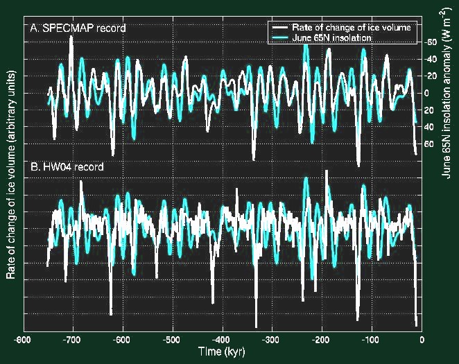

Both Science of Doom and I have discussed it and replicated it, although in our replications we we used the newer data rather than the older data used by Roe. As SoD pointed out, the top panel above (SPECMAP) used “ice volume” data that was tuned to the insolation, so it is useless.
So let me refer you to SoD’s excellent discussion, here and here, to which I have little to add.
Please note the only differences between the lower panel above and my Figure 3 in the head post are that 1) I’ve inverted the ice volume proxy data (so that warming is up); 2) I’ve used the newer Huybers data as a proxy for ice volume rather than the Huybers 2004 data used by Milankovich; and 3) I’ve used the Berger insolation data, which is slightly different from that used by Milankovitch. (The only provenance of the insolation data used by Milankovitch is “The author thanks J. Levine for providing the insolation codes”, or I would have used Milankovitch’s insolation data.) Here is my data, in the format used by Milankovitch:
In other words, I’ve repeated the Milankovitch analysis used in the lower panel. As a result, all of the figures and calculations are of the Milankovitch claims, replicated using the best and most modern data that I can find.
Regards,
w.
Willis,
In Fig. 1, you are comparing an “energy flow” variable (J/s/m^2) and a “scalar state” variable (deg C), and you’re plotting them on a time-logarithmic scale. That means that those tiny bumps near 100ky in the red curve of Fig. 1 actually correspond to 10,000s of years of having a somewhat higher influx of energy; in total, quite a lot of extra energy. The big peaks at 20 and 40 years look more impressive, but correspond to much less energy being sent to the earth. So is it entirely fair to compare the two? Basically, all the signal power near the 100ky frequency is spread over a much wider interval.
Would it not be interesting to have a binning of signal energy, e.g. add all the peaks from 0-999 into a bin, and rinse and repeat for 1000-1999, …., 100000-100999, etc., and then plot the binned signal against the average temperature over that bin?
Frank
Willis –
I wouldn’t argue that insolation at a specific latitude forces global temperature. You are on the right lines in suggesting now that temperature first differences should relate to insolation, especially when the ocean is going to take thousands of years to equilibrate at depth, i.e. response to insolation is not instantaneous.
However, the multiple orbital parameters clearly do provide a very helpful model, when you consider:
oops. When you consider:
1. Changes in *Global* insolation, forced by eccentricity changes
2. Changes in Obliquity, dictating the size of the arctic/antarctic zones
3. Changes in Perihelion, dictating the relation between the seasons and the earth’s orbit.
All of these together can generate quite a fetching fit to global temperature.
If you are trying to debunk the idea that insolation at a specific latitude drives ice ages, I’m right with you. If the broader point is that an explanation based on (Milankovitch) orbital parameters is wrong, then I think that isn’t the case. As posted before, see:
http://www.robles-thome.talktalk.net/Milank1.pdf
R.
In the geological past there was a prolong period when the Earth’s poles were free from the long term ice coverage, followed by the current glacial epoch. The cause of the change from one to the other is not clear, possibly the solar system’s passage through galactic dust clouds.
However, what is clear is that the short irregular interruptions of the glacial epoch are correctly identified by the Milankovic cycles of increase in the N. Hemisphere’s solar irradiation
As these short periods in steep temperature rises are irregular spectral analysis will not lead to correct interpretation of periodicities concerned.
Finally, the absence of the Dr. Svalgaard’s comments is regrettable.
May I summarise the comment I made in the last thread.
The pattern can be explained if one assumes the following
1) The onset of an ice age is caused by reduced insolation (MC)
2) Ice growth is accelerated by albedo changes
3) Sea ice reduces the energy lost to space so that the energy balance is POSITIVE which means that energy is stored in WARNING oceans under the ice.
4) The warming oceans melt the ice from below as the ice thickens above creating huge instability in the ice shelves
5) Eventually the sea ice calves into the warm oceans creating relatively rapid temperature fluctuations as the ice packs melt in the summer exposing the warm oceans and refreeze during the winters restoring the ice cover until the next major calving.
This pattern began to appear a couple of 1 million years ago when the Isthmus of Panama closed and became fully established 1 million years ago once the Atlantic had cooled to a critical temperature. Prior to this the Atlantic was warmed by currents and winds from the Pacific which prevented massive sea ice build up.
CAL
This is a very helpful summary, and explanation of ice sheet instability. An action causing its own reaction – this can be called “friction” and is a necessary ingredient in chaotic-nonlinear instability and oscillation.
About the Atlantic and Pacific. In Willis’ previous Argonouts post, the temp with depth animation showed that the Pacific at depths >1000m is colder than the Atlantic (and Indian) ocean. So the Atlantic is cooler at the surface but warmer at depth, than the Pacific. Is there a zero sum game here? With the heat capacity of water, and the volume of water in the oceans, there must be in the short term.
Frank Excellent point
Combine Franks comment at 4:32 1/26
“In Fig. 1, you are comparing an “energy flow” variable (J/s/m^2) and a “scalar state” variable (deg C), and you’re plotting them on a time-logarithmic scale. That means that those tiny bumps near 100ky in the red curve of Fig. 1 actually correspond to 10,000s of years of having a somewhat higher influx of energy; in total, quite a lot of extra energy. The big peaks at 20 and 40 years look more impressive, but correspond to much less energy being sent to the earth. ”
with Denniswingo at 7:18 pm 1/25 who points out
” Look at first principles. At maximum eccentricity the difference in insolation at the top of the atmosphere is well over 100 watts/m between perihelion and aphelion. That is a hell of a difference. Using average values masks these variations.”
I think this provides an explanation of the eccentricity influence.
Willis,
about the “solution” of this 100ky cycle problem (one of the many solutions), you should definitely check out Abe-Ouchi et al 2013 Nature Vol 500 Nature 8 august 2013
http://www.nature.com/nature/journal/v500/n7461/full/nature12374.html
Further to my comment immediately above. The oceans have a volume of just over 1Billion cubic Kilometres. Assuming the peak ice was about 10 million cubic kilometres and a latent heat of ice of 340 joules per gram the melting of the this volume of ice would reduce the global sea temperature by 3 degrees centigrade. Or putting it another way the pattern would be consistent with the sea taking about 80,000 years to increase by 3 degrees and then 20000 years for it to cool down again as the ice melts. In my mind this sort of time constant is not unreasonable.but it would be pretty inconsistent which explains why the average periodicity is constant but the actual value is not.
How about over 50million km^3 Cal? I commented above that a couple of simple things being missed by all commenters including Willis I believe, is at peak glacial thickness, the low humidity means little or no more accumulation, but sublimation of the ice into the low humidity is a likely significant happening. Remember, even if insolation increases, much of the glacier is a couple of km thick and thus is a topographic high, like the ice on top of a mountain even in mid july. Now sublimation could probably take 50,000 years to reduce the ice to a point were insolation matters a lot more. Of course, gravity flow of the ice is also removing mass from the highs, probably faster as warming begins to have an effect.. .
Willis. Run the numbers. I challenge you. Do the insolation at perihelion and aphelion during minimum eccentricity periods vs during maximum eccentricity periods. Your response will be that it averages out, but that is not the point, it is the seasonal values that are important and when you have the northern hemisphere at aphelion during maximum eccentricity, and with the albedo of the land, and the altitude of the Northern Hemisphere thrown in, that is a major difference in energy input into the system.
There are papers out there that explain this but if you are not willing to listen then just continue to scratch your head.
My friend, that’s your theory, not mine. So I invite you to run the numbers, graph up the results, and come back and present your graph. Note your methods and data sources, please, so we can all understand what you’ve done.
I look forward to your results,
w.
Apropos ‘Milankovitch can’t explain 100K year cycles’, check out the first chart on page 2 of my paper.
http://www.robles-thome.talktalk.net/Milank1.pdf
The total earth insolation has a strong periodicity around 100K years driven by changes in eccentricity.
R.
Willis
I don’t really care that much about it, after doing a lot of research and looking at the data, I am convinced of the 100k orbital forcing, though we don’t have the exact explanation for it. Here are a couple of papers for your interest. I see the difference of about 80 watts/m2 in my satellite data for a year and that is at our low eccentricity of the modern era. At 120-140 watts/m2 at high eccentricity that is all I need to figure it out.
https://www.dropbox.com/s/yimaqatvjh0l9ny/Vostok_420k_CO2.pdf?dl=0
This is the best paper below on long term eccentricity. It may change your calculations because most use an older paper for it (Lasker 1990). Here is a question for you. Do you know who’s work your insolation calculation is based on for eccentricity? Hint: it matters.
No one knows what the driver is but everyone agrees that except for 400k years ago, the orbital eccentricity data best fits our recent ice age periods.
https://www.dropbox.com/s/yfhjreodgrwqhf9/Earth_eccentricty.pdf?dl=0
RERT January 26, 2015 at 2:12 pm
RERT, as your chart shows, the change in insolation due to insolation is a whacking great 0.4 W/m2. On my planet, that’s called an “extremely weak periodicity”, not a “strong periodicity”, and that’s exactly the problem. It’s far too weak to kick the earth either into or out of an ice age.
w.
dennis said:
denniswingo January 26, 2015 at 9:32 am
I replied:
Willis Eschenbach January 26, 2015 at 12:31 pm
dennis says:
denniswingo January 26, 2015 at 3:01 pm
Cute, dennis. You challenge me to do your work for you, and when I decline, you say you don’t really care, and you don’t have any facts … but by gosh, you’re convinced anyhow.
You see why I don’t let folks direct my research? If you don’t care enough to do the work, why should I?
Sorry, but after that little trick, dennis, I’m not interested in the slightest.
w.
—Willis
I don’t really care that much about it, after doing a lot of research and looking at the data, I am convinced of the 100k orbital forcing, though we don’t have the exact explanation for it.—
Well I would say it related to ocean warming and cooling- though that not an exact explanation.
Or temperate glacial advance and retreat is just a symptom rather than causal factor.
Anyways I not sure what causes Earth’s change in eccentricity- I assume some kind a resonance with Jupiter and/or other planets- but that’s about it.
I wonder if the sun is dragged and so Earth follows- [and so all the inner planets] whether planets
changing independently.
So:
“The shape of the Earth’s orbit changes from being elliptical (high eccentricity) to being nearly circular (low eccentricity) in a cycle that takes between 90,000 and 100,000 years. When the orbit is highly elliptical, the amount of insolation received at perihelion would be on the order of 20 to 30 percent greater than at aphelion, resulting in a substantially different climate from what we experience today. ”
http://earthobservatory.nasa.gov/Features/Milankovitch/milankovitch_2.php
Seems to indicate the the earth just moves closer to the Sun.
And does not say earth move further away from Sun at aphelion. If true that indicates earth orbit lost energy [and then is suppose gain energy??}.
If just the earth perihelion moved nearer, then it would be more “obvious” to all that changes climate. And would guess that is what writer of above article is assuming.
If the sun moved instead earth orbit does need to gain or loss orbital energy, and 365 day orbit would seem to be maintained.And also it’s “less obvious to all” that causes climate change. I think it would, but I am not greenhouse effect theory believer.
So what are the orbital perimeter- the perihelion and aphelion that earth is said to change every 90 to 100 thousand years?
So sort of answering my questions.
“Right now, the elongation of the orbit (the eccentricity) is rather small — about 1.7%. This results in the sun being about 7% brighter at the earth when it is closest, on January 4, than when it is most distant.
Twelve thousand years ago, when the glaciers of the last great ice age were melting, the eccentricity was a bit higher, about 2%. At the same time, the earth was closest to the sun in June, and most distant in January, so the sun was about 7 % brighter in June than it is today.”
http://www2.gi.alaska.edu/ScienceForum/ASF8/825.html
Average earth orbit is 149.6 million km. Times by 1.017 [1.7%] gives our Aphelion of 152.14 million km. And divide by 1.017 gives our Perihelion of 149.09 million km.
So instead 1.7% it’s 2%:
Perihelion: 146.66 and Aphelion of 152.59 million km
Next:
“During the interglacial before the last ice age, about 125,000 years ago, the eccentricity was about 4%. The times of largest eccentricity tend to be about 100,000 years apart.”
So instead 1.7% it’s 4%:
Perihelion: 143.85 and Aphelion of 155.58 million km
So as we know the last interglacial was warmer than our current interglacial.
Oceans About 2 C warmer and sea level 6 meters higher [or somewhere around there]
So another quote from article:
“At various times in the last million years, however, the eccentricity has been much higher — as much as 6%, which would make the sun almost 25% brighter at perihelion (when the earth is closest to the sun) than at aphelion (when the earth is farthest from the sun).”
So instead of 1.7% it’s 6%:
Perihelion: 141.13 and Aphelion of 158.58 million km
So that is maintaining the 365 day year [I believe] and if true, my guess [currently] is the sun
moves [rather than earth [mostly moving]- because it seems simpler.
But I mean mostly the sun moves [or certain both move- but my question was which moves more].
So it seem if Earth has shorter Perihelion Earth gets a warmer ocean. Or at least it does when Earth is in a Ice box climate.
Oh, here calculator for Eccentricity of the orbit of the Earth for 1 million BC to 1 million AD:
http://www.jgiesen.de/kepler/eccentricity1.html
Your loss. The second paper is the best one I have seen for putting together the insolation numbers derived from an analysis of the orbits of the major planets in the solar system. They have an interesting difference from previous numbers. I bet you don’t even know who’s numbers you are using for the eccentricity term. Guess what, they have changed significantly as a result of the paper I provided.
So, I provide you with the best paper on the subject, which you requested research that I don’t have to do, and you reject it. Neat….
Science is a lot more than just grabbing the first thing that is out there, crunching some numbers, and declaring victory.
denniswingo January 27, 2015 at 8:19 am Edit
Well, against my better judgement I went to look at your whiz-bang paper. It says right up there in the abstract:
In other words, guess what? For the period under discussion (within the last million years), the paper you think is so all-fired important doesn’t make one damn bit of difference … why am I not surprised?
It was neat, and I should have stuck to my guns, because the paper was useless.
How would you know? I asked you to do a bit of science regarding your own claim and you refused. So I did your work, I took a look at your recommended paper and found out that your claim that the numbers have “changed significantly” only applies to a period of time that is not under discussion.
In other words, you just grabbed the first thing that is out there, you didn’t even bother crunching some numbers, and you declared victory …
Neat …
w.
–Willis Eschenbach
January 26, 2015 at 12:31 pm
My friend, that’s your theory, not mine. So I invite you to run the numbers, graph up the results, and come back and present your graph. —
–Willis
I don’t really care that much about it, after doing a lot of research and looking at the data, I am convinced of the 100k orbital forcing, though we don’t have the exact explanation for it. —
To sum it up.
There is no theory which allows us to exactly explain the past climate, and thereby enable anyone to predict the future.
For example we have climate record going back hundreds of thousands of years, which is not random but instead has a somewhat clear pattern to them. The orbital changes of Earth appear they could provide explanation of this pattern, but there is not a known way to do this.
So the fairly well known changes of orbital characteristics of the past and fairly well know orbital changes which will occur in the future, are not currently helpful to predict the future of earth climate.
The climate record itself is more predictive of the future climate than milankovitch cycles which attempts to explain them. Which is to say our climate record give a clue that within thousands of years we could return to glacial conditions and the milankovitch cycles/earth orbital characteristics do not help clarify this.
So at this point, have to say the milankovitch cycles do *not* help explain why our last interglacial
was warmer [despite my earlier assertion] , nor I am able to explain how it effects our current interglacial.
I can’t say what the effect of orbital changes have, though they seem they *should* or *could* have a large effect.
Or I would say the changes in earth orbital characteristics are clue, but then again we seem to have many clues.
And it appear most relevant issur to me at the moment about the near term future is that we had more than century of ocean warming and departure from the Little Ice age, and this probably will continue to be the case for next 50 years or more. And that solar activity in next couple decades will probably be lower than has been for a 100 years, and I expect the 18 year pause to continue for next 5 to 10 year. And none of this has anything to do with milankovitch cycles.
[And in next 5 years I expect CO2 levels to rise to about 410 ppm and this rise will continue to have unmeasurable effect upon global temperatures. And polar sea ice will not completely melt, the polar bears are doing ok, and of course, Obama has actually done nothing to stop the sea from rising.]
The albedo causing or triggering Glacial periods is only another such figment..
Whiten says to me.
My reply
Which is not what I am trying to convey. What I am trying to convey is not a change in albedo triggering glaciation. What I am trying to say is why does the POSITIVE FEEDBACK between an increase in snow cover/ice cover which will result in a higher albedo hence colder global temperatures does not feed upon itself once it gets established? One would think it would with all other things being equal but this is not the case.
The question is what is it that causes this not only not to happen but reverse ?
I can not get away from the notion it must be tied up with solar variability and the associated primary /secondary effects associated with this variability.
Anyone have any other possible explanations?
The problem with Milankovitch cycles is two fold ,first glaciation occurs in both hemispheres at the same time and secondly the abrupt climatic changes are far to rapid and occur far to often in order to be explained by the very slow Milankovitch Cycles.
Ice core data shows evidence of the earth transitioning from inter-glacial to glacial conditions in decades . I have come up with some thoughts on this in my earlier post.
The YOUNGER DRYAS – that event alone is a nail in Milankovitch Cycles as the prime mover of the climate.
That said I do think Milankovitch Cycles have a back-ground role in the climate variability but only that.
I could even see how the S.H. could cool even when Milankovitch Cycles favor warming there, due to the N.H. cooling /increase albedo, over powering the globe as a whole.
Salvatore The weight of evidence suggests that the rapid cooling of the YD and 8200 year events are caused by comet impacts – they have no relation to Milankovic cycles.
4) The warming oceans melt the ice from below as the ice thickens above creating huge instability in the ice shelves from CAL
My Reply
What factor or explanation do you have to explain why all of a sudden, in an increasingly colder higher albedo world, the oceans all of a sudden start to warm? What happened to bring that on?
The oceans do not suddenly start to warm. They gradually warm as a result of the very low cloud cover because of the low humidity bordering the ice caps. Thus the equatorial waters receive huge amounts of energy. Instead of flowing north and radiating energy at most latitudes south of the arctic circle they flow north under the ice. This prevents radiation to space. There is strong evidence that the Baltic sea was indeed warm under the ice.It is this lack of radiation to space that causes the positive radiation balance and the gradual warming.
However, what is clear is that the short irregular interruptions of the glacial epoch are correctly identified by the Milankovic cycles of increase in the N. Hemisphere’s solar irradiation. Vuk says
My reply
Wrong , and all one has to do is look at the historical climatic record 22,000 to 10,000 years ago to see the many abrupt climatic changes are in no way related to the very slow Milankovitch Cycles.
If the first difference makes a better correlation, then does using the second difference, which will de-emphasize the 100kyr cycle with respect to those at lower period even more, help the correlation further? In other words, is it the case that rate of change of the rate of change of temperature, or ice volume, is what the orbital elements drive? I’m not a fan of continuing down such a path, I’d rather have an understanding of actual physics drive the analysis, rather than transform the input in various ways to improve correlation.
There is a explanation of the 100kyr problem in the data, however. The figure doesn’t place a peak at 100kyr in the insolation periodogram, but there is power at 100kyr. So, let’s think of the climate as a linear black-box system. If Delta-T/Delta-I is admittance, at 100kyr the admittance is very large. The transfer function has a pole, with high Q, near 100kyr. Why? I don’t know–some combination of climate force and inertia, or feedback, or lag in the system. But my point is, as long as some some power exists at 100kyr in the insolation periodogram, there is a basis for explaining the 100kyr temperature swing using it.
http://wattsupwiththat.com/2013/06/02/multiple-intense-abrupt-late-pleisitocene-warming-and-cooling-implications-for-understanding-the-cause-of-global-climate-change/
Milankovich cycles can NOT explain these abrupt climatic changes which means it is not the main reason for why the climate changes. It is that clear cut..
Feedback, and momentum! R.
Dr. Norman Page I doubt that is the reason and even if it was how do you explain all of the other abrupt climatic changes which I just posted? It is by no means limited to the YD or 8200 year cold period. There are countless other abrupt climatic changes besides those two. It is very unlikely that impacts were the cause.
To make it even more unlikely it was some sort of impact it is not just the beginning or ending of the YD but all of the abrupt climatic changes within the YD.
I would say the impact theory has a 0% chance of being correct.
Salvatore Just eyeballing roughly the number of peaks between 11500 and 13000 it looks very much like the good old 60 year cycle ( see following comment) also there is no scale on the graph to show the amplitude of the cycles.
It is obvious that the glacial cycles are Milankovic related .
The evidence for impact at the beginning of the YD is substantial. The evidence for impact at the beginning of the 8200 year event is certainly much less than for the YD.
There is clear evidence for solar activity quasi periodicitiesin the Holocene For the 1000 and 60 year periodicities seen in the temperature data. see Figs 5-9 and 15-16 at
http://climatesense-norpag.blogspot.com/2014/07/climate-forecasting-methods-and-cooling.html
The solar driver connection to temperature is shown in the relations between Fig 9,10 C,D 11 and 12.
The reasons why we are just past the millennial cycle peak are seen in Figs 13 – 14.
and the millennial cycle trend peak at about 2003 is seen in the graph
http://www.woodfortrees.org/plot/rss/from:1980.1/plot/rss/from:1980.1/to:2003.6/trend/plot/rss/from:2003.6/trend
As a limited test of this approach I am suggesting a significant cooling in 2017- 18 based on the sharp Ap index break at 2005-6 in Fig 13.
It is also clear that particularly during glacial and cooler periods the climate is in a state of unstable equilibrium so that small changes in some variable eg volcanic activity can cross some threshold and trigger rapid temperature changes,
Dr. Page my reply to you.
I do not agree entirely with your explanation as to why/how the climate changes. Some of your thoughts I do agree with.
I am more in the camp of Don Easterbrook as far as why Milankovtich Cycles influences on the climate but not exactly 100%.
Like yourself I expect cooling going forward but primarily from solar variability and the primary and secondary effects associated with this solar variability. Again I know you feel this way to some extent also. I think however I emphasize solar variability as having a bigger role in the scheme of things then you do.
From Don Easterbrook – Aside from the statistical analyses, there are very serious problems with the Milankovitch theory. For example, (1) as John Mercer pointed out decades ago, the synchroniety of glaciations in both hemispheres is ‘’a fly in the Milakovitch soup,’ (2) glaciations typically end very abruptly, not slowly, (3) the Dansgaard-Oeschger events are so abrupt that they could not possibility be caused by Milankovitch changes (this is why the YD is so significant), and (4) since the magnitude of the Younger Dryas changes were from full non-glacial to full glacial temperatures for 1000+ years and back to full non-glacial temperatures (20+ degrees in a century), it is clear that something other than Milankovitch cycles can cause full Pleistocene glaciations. Until we more clearly understand abrupt climate changes that are simultaneous in both hemispheres we will not understand the cause of glaciations and climate changes.
My reply
All the above which is what the data shows lends support to my thoughts that solar variability and the primary and secondary effects associated with this solar variability are a big player in glacial/inter-glacial cycles when taken into consideration with these factors which are , land/ocean arrangements , mean land elevation ,mean magnetic field strength of the earth(magnetic excursions), the mean state of the climate (average global temp), the initial state of the earth’s climate(how close to interglacial-glacial threshold it is) the state of random terrestrial(violent volcanic eruption) /extra terrestrial events (super-nova in vicinity of earth or a random impact) along with Milankovitch Cycles. These factors setting the back ground for a general climatic trend for the earth to move in if solar variability did not exist at all.
What I think happens is those factors keep the climate of the earth moving in a general trend toward either cooling or warming on a very loose cyclic or semi cyclic beat but get consistently interrupted by solar variability and the associated primary and secondary effects with this solar variability which brings about at times counter trends in the climate of the earth within the overall trend , or at other times when all the factors I have mentioned setting the back ground for the climate trend for cooling or warming along with what solar variability has been doing or a random terrestrial /extra terrestrial event (which can explain some of the dramatic climate changes maybe 10%of them) in conjunction with these factors( which are land/ocean arrangements, mean land elevation ,mean state of the climate and initial state of the climate, Milankovitch Cycles) , then drive the climate of the earth gradually into a cooler/warmer trend(unless it is a random terrestrial or extra terrestrial event in which case it would be rapid even if the climate initially is far from the glacial /inter-glacial threshold ) UNTIL it is near that inter- glacial/glacial threshold or climate intersection that makes any further solar variability no matter how slight at that point to be enough to cascade the climate into an abrupt climatic change. The back ground for the abrupt climatic change being in the making all along but when the threshold glacial/inter-glacial intersection for the climate is reached that is NOT ONLY when the abrupt climatic changes occur but the constant swings in the climate from glacial to inter-glacial over short periods of time can take place .
The climatic back ground factors along with the general trend in solar activity driving the climate gradually toward the climate intersection or threshold of glacial versus interglacial, then once there at the intersection the climate gets wild and abrupt. Although random terrestrial events and extra terrestrial events could be involved some times to account for some of the swings in the climatic history of the earth but not all of them ,maybe 10 % of them.
The climate is chaotic, random and non linear but in addition is never in the same mean state or initial state which makes given forcing to the climatic system not resulting in a given outcome which is why I think there is a semi cyclic nature to the climate but it is consistently being disrupted with counter- trends at times or abrupt changes at times.
If what I say is not on the correct path then why is it whenever the climate strays from its mean in either a negative or positive direction it is ALWAYS brought back to its mean. Why does the climate never go in the same direction once it heads in that direction?
Why is it that when the ice sheets expand the higher albedo /lower temperature more ice expansion positive feedback does not keep going once it is set into motion? What causes it not only to stop but reverse?
Vice Versa why is it when the Paleocene – Eocene Thermal Maximum came about that the increase CO2/higher temperature positive feedback not only did not keep proceeding but reversed?
.
Like I said before, this graph is sufficient proof for M cycles as the driver: http://en.wikipedia.org/wiki/Milankovitch_cycles#mediaviewer/File:Vostok_420ky_4curves_insolation.jpg
R is next to meaningless: does it vary according to the number of cycles of correlation? Each additional cycle of correlation multiplies the unlikelihood of spurious correlation. And of what use is lag analysis if the lag varies between each cycle, according to variably sized ice caps? How can albedo be taken into account? It’s all reminiscent of the denial of the statistical force of Wegener’s observations.
To melt 1km of ice in 10ky requires 3w/m^2 (average). M cycles are quite capable of delivering it, or not. Not all the ice is a mile thick; thinner ice at lower latitudes can melt in a hurry: http://www.nature.com/nature/journal/v502/n7473/full/nature12609.html
…causing a step change in albedo to add to growing insolation. All the ice has to do is melt faster than it snows. Not even that, really. All that is needed is for snow to change to rain. –AGF
Salvatore I agree that for forecasting climate on time scales of interest to civilization ie the next 1000 years the solar driven quasi-millennial cycle seen in the temperature data is key. As to the processes involved I say
in the link above
“NOTE!! The connection between solar “activity” and climate is poorly understood and highly controversial. Solar “activity” encompasses changes in solar magnetic field strength, IMF, CRF, TSI, EUV, solar wind density and velocity, CMEs, proton events etc. The idea of using the neutron count and the 10Be record as the most useful proxy for changing solar activity and temperature forecasting is agnostic as to the physical mechanisms involved.
having said that, however, it is reasonable to suggest that the three main solar activity related climate drivers are:
a) the changing GCR flux – via the changes in cloud cover and natural aerosols (optical depth)
b) the changing EUV radiation – top down effects via the Ozone layer
c) the changing TSI – especially on millennial and centennial scales.
The effect on climate of the combination of these solar drivers will vary non-linearly depending on the particular phases of the eccentricity, obliquity and precession orbital cycles at any particular time.
Of particular interest is whether the perihelion of the precession falls in the northern or southern summer at times of higher or lower obliquity.”
It is simply not necessary to understand all the problems of the beginning end of the ice ages and the temperature variations during glacial episodes or the PETM in order to make perfectly reasonable forecasts for the next 1000 and especially for the next 100 years. These matters are of important academic interest but the state of the system as a whole during those events was very different from the present and are of limited relevance to forecasting the next thousand years.
If we can understand Fig 5 at
http://climatesense-norpag.blogspot.com/2014/07/climate-forecasting-methods-and-cooling.html
that is really all we need- at least if our main interest is forecasting the next 1000 years.
Salvatore Check my 2:21 comment.
I suspect that the continental ice network has a clock frequency of 1 / 100K years.
I think we agree in principal.
I think one difference is you see the climate as more cyclic ,I see it as being semi cyclic with a random pattern superimposed upon the semi cyclic pattern . I also think I put much more evidence on the initial state of the climate to attain a given climate result then you do.
I am of the opinion that much more information is going to be coming forth about solar/ climate connections and variability of the sun as this prolonged solar minimum period extends.
Look at my post jan 25th at 11:23am
The key will be the neutron count at the next solar minimum (count maximum) in about 2021. If it peaks significantly above the 2009 count, temperatures will really be heading down for the following 15 years at least and I will have more confidence in my 2035,2100 and 2600 forecasts.
that we agree on 100%
Willis,
here is a paper that should interest you: The Albedo of Earth,
http://onlinelibrary.wiley.com/doi/10.1002/2014RG000449/abstract?campaign=wolacceptedarticle
Send me an email if you need a copy.
They show that Earth’s albedo is amazingly constant in time and between hemispheres. The GCMs do not capture this at all.
Interesting, but not relevant to the question of M cycles. –AGF
I take that back: if clouds disperse with growing sea ice, I suppose the same could mysteriously happen with land ice.
Thanks, Matt. I’d noted and commented on that in my investigations into the CERES data. Do you have a citation for the inability of the GCMs to capture this oddity?
w.
Salvatore
I can not get away from the notion it must be tied up with solar variability ..
No you cant, and this is looking more and more problematic. To say “everything imaginable in climate can only be caused by one thing – direct response to solar changes – and nothing else” is very similar to saying “everything imaginable in climate can only be caused by one thing – direct response to CO2 changes – and nothing else”.
Disputing Milankovich pacing of the glacial cycle is the same as disputing Galileo and Copernicus and trying to thread-bomb us all back to epi-cycles. From 1-3 million yrs ago interglacials were paced by 41 kyr intervals, the length of the obliquity cycle. After than (the MPR) the pacing changed to 100 kyrs – the eccentricity cycle. An orbital pacing signature is hard to deny (although that’s clearly not stopping you from trying).
Note I use the word “pacing” and not “forcing”. The climate is a chaotic-nonlinear system. Again, no amount of thresdbombing will change this fact. The AGW crowd imagine climate to be passive and driven by CO2 radiative forcing. You believe the climate to be passive and driven by solar forcing. You are both wrong. Climate is dynamic and drives itself (its more than 18 years old!) BUT – nonlinear oscillators CAN be periodically forced from the outside. This can be strong forcing, where the forcing frequency is reflected in the driven system. But it can also be weak forcing – where the responsive oscillation timing is related only in a very complex way to the forcing frequency. I strongly believe that the role of solar fluctuations, since the percent changes in energy are so small, is weak periodic forcing. Milankovich cycles are also a combination of strong and/or weak forcing. In fact the “Mid Pleistocene revolution” or change from 41k obliquity pacing to approximately 100 kyr pacing may well represent a transition from strong to weak nonlinear periodic forcing.
Climate study will only emergy into the sunlight and stop wasting time when it acknowledges fully the chaotic-nonlinear character of the system and all its implications.
FYI, processing André Berger’s insolation data is somewhat of a pain because the files are split up into tiny 144k chunks. Most likely an ‘artifact’ of the early 1990’s when he generated these files and floppy diskettes were restricted in capacity to 720kb:
http://www1.ncdc.noaa.gov/pub/data/paleo/climate_forcing/orbital_variations/berger_insolation/
But now there’s a much easier way to generate this same data in R using the ‘palinsol’ package, which was written by Berger’s protegé, Michel Crucifix at the University of Louvain in Belgium:
http://cran.r-project.org/web/packages/palinsol/palinsol.pdf
Just use the ‘install packages’ tool in R to install it. (But you’ll need the latest version of R, ver3).
I wrote a little script to generate the same 0-800kyr range that Willis used.
The palinsol package actually computes the insolation, from computed solar system orbitals and perturbations, using Berger’s very detailed algorithms. You can select either the 1978 or 1990 versions of the code. The 1990 version used more terms in the regression and corrected some minor errors in planet masses etc. But for the first 1.5 million years the outputs are the same. So I used the 1978 version.
My script also computes the periodogram of the data using the ‘spectrum()’ function in R (right panel)
http://i62.tinypic.com/5agm6p.png
Note that the spectrum is logarithmic, not linear like Willis’. So the data looks more compressed. Also there are more peaks. Probably because I didn’t smooth the data. (But there is a default 0.1 cosine taper applied by the spectrum() to suppress some of the sync() side lobes)
So I think it captured all of the signals that Willis saw (and more), but it didn’t generate a signal at 2kyr, which I think may be aliasing, as noted by others earlier. I zoomed the plot a bit and used the locator() function to extract the 16 largest peaks (marked with red +’s)
http://i59.tinypic.com/2bbrli.jpg
http://i58.tinypic.com/htu0ps.png
Disregard the decimal precision of these numbers, because they depended on my manual dexterity while positioning the +’s. They’re probably off by 5% or so, but close enough for ‘government work’.
Note the 100kyr signal is there and looks pretty large in the log plot. But its true intensity is less than 5% of the procession peaks at 23.3kyr. So comparable with Willis’ results.
But I’m curious why Willis’ plot doesn’t show the 400kyr wave, which is readily apparent, even in the time domain plot.
Here’s the R script to generate this plot and data: 801 samples, 1 per kyr, from 0 to 800kyr BP
#————- mysol.R ——————-
require(palinsol)
require(graphics)
insolation = function(times, astrosol=ber90,…)
sapply(times, function(tt) Insol(orbit=astrosol(tt)))
tts = seq(from = -800e3, to = 0, by = 1e3)
isl = insolation(tts, ber78)
par(mfrow=c(1,2))
plot(tts, isl, typ=’l’, main=’berger78: -800ky to Present’)
spectrum(isl,main=’Spectrum: freq.res=1/1602kyr period.max=2kyr’)
grid()
n=16
loc=locator(n)
text(loc, ‘+’,col=’red’)
print(1/loc$x[1:n])
print(sqrt(loc$y[1:n]))
I said:
“…didn’t generate a signal at 2kyr, which I think may be aliasing, as noted by others earlier. ”
Upon reflecting further, I don’t think it’s aliasing, because that always starts at the low-frequency end of the spectrum, and 2kyr is the very highest frequency possible in this sampling regime.
So there must be some other reason I don’t see any significant energy at 2kyr comparable to Willis’ plot.
Johanus said: “Upon reflecting further, I don’t think it’s aliasing, because that always starts at the low-frequency end of the spectrum.”
There is obviously “high frequency” content in temperature data. There was a larger temperature range here today from morning to afternoon (one cycle per day) than in all of the subject data. Thus, aliasing error is certainly possible. There is likely some sort of natural low pass filtering of this in the ice core generation and analysis process, but it’s characteristics are unknown, at least to me. A perfect boxcar shaped filter would allow all of the Nyquist frequency content (one cycle per 2000 years) through, and completely eliminate all other higher frequencies. This would be highly unlikely for any number of reasons. So lets assume there is some sort of realistic, likely single pole, low pass filter, present in the original ice core generation process.
If there were such a realistic filter, and if there were also no aliasing errors, there would be no content at the Nyquist frequency. The filter would eliminate it in the process of eliminating other aliasing error. The fact that there is, at least in Willis’ chart, means that there are some aliasing errors present in the data. With broadband white noise data, and properly selected multi-pole anti-aliasing filters, the largest aliasing error occurs at the Nyquist frequency, and reduces for lower frequencies. Since the data are not white and the high pass filter is likely not multi-pole and certainly not “properly selected”, the aliasing errors are likely to be at any of the frequencies in the chart.
Tom:“There is obviously “high frequency” content in temperature data. “
But this is about the Berger insolation dataset. There is no ‘temperature’ data in that. It’s all synthetic astronomical data, generated from orbital mechanics.
Willis’ periodogram of the Berger data (red trace) had a 2kyr ‘bump’ which did not show up in my equivalent periodogram generated from palinsol data.
Oops. I was thinking of the wrong data. There may or may not even be an issue with aliasing, depending on the method of generating and of reading the Berger insolation data.
Johanus, thank you so much for your link to the marvelous R package, and also for posting your R code. Very neat.
Also, the reason I don’t show the 400 kyr cycle is that I was working with only only 1,000 kyrs of data, and I cut off any such analysis at a third of the length of the data.
I believe that what you’ve found is an artifact of the short time span. I just tested it by looking at 1,600 kyr of the Berger78 data, and there’s no significant 400 kyr cycle.
w.
Thanks.
“I just tested it by looking at 1,600 kyr of the Berger78 data”
I did the same with my script using this statement to expand the times sequence to 1600kyr:
tts = seq(from = -1600e3, to = 0, by = 1e3)
The resulting plot still shows the 400kyr spectral line and a new one at 1.2 myr. I think these are “real” signals (in the synthetic data, heh).
You can actually “see” a 400kyr wave in your time domain plot (with peak amplitudes at -600 and -200 kyr):
PHLOGISTON – if you read my recent post you would see that what I am saying is very similar to what you have said.
The only difference is I believe solar variability is a bigger player in the overall climate scheme of things then you do.
First, why should the 60th or 65th parallel temperature matter? Why not the 40th or 45th parallels where most glaciations stopped?
Second, 100Kya is an average and you should know better than to pin an argument on a mathematical construct that doesn’t reflect a multi-dominate mode. The modes of ice ages run at 82 and 123 kyrs. The use of average or mean leads to false conclusions when the mode is so strong. You’re making the exact same mistake as taking the average temp of the Northern Hemisphere and Southern Hemisphere to come up with the GAT. The volatile NH overrides the SH stable temperature paradigm giving the false idea that the WHOLE of the planet is heating when only part of it is.
Third, you make the assumption using the Milankovichcycle that obliquity change is constant throughout the cycle. Does it not occur to you that when the ocean level drops 450 feet during the depth of the ice age that weight is mostly redistributed from the water dominated SH to the land dominated NH? Do you honestly believe there is ZERO impact on the rate of obliquity during the ice accumulation phase and the melting phase when so much weight is redistributed from South to North?
A couple of interesting excerpts from posts.
This one from “Ask a scientist UK”
Question “What caused reduction in CO2 leading to the ice ages?”
Answer by Michael de Podesta April 27, 2012:
“It’s a great question, but does not have a simple answer. There are two parts to the answer and to understand these I need to ask you to distinguish between the ‘trigger’ events which started the transitions into and out of ice ages and the ‘drivers’ which kept the change going
Trigger: We believe that triggers for the ice ages and interglacial warming periods are small changes in the attitude of the Earth in its annual journey around the Sun. These ‘orbital wobbles’ are small and barely alter the average amount of energy reaching the Earth. But they do alter day length and summer length at high latitudes. Imagine what happens at the ‘snow line’ – the line of latitude at which snow just lies on the ground over summer. If summer lengthens or intensifies then this can cause snow to melt, which changes the albedo of the surface – making it darker and increases the rate of warming. Orbital changes trigger this kind of change.
Driver: When the Earth warms up microbes wake up and digest biological matter in the Earth and release methane (CH4) which reacts after about 10 years to make CO2 which stays in the atmosphere for hundreds of years – causing more warming and making the release of further CO2 more likely. So the ice core record shows changes in CO2 that correlate with ice ages. But these did not trigger the ice ages or interglacial periods. However, the changes in CO2 concentrations did drive the changes once they began.”
http://askascientist.co.uk/chemistry/what-caused-reduction-in-co2-leading-to-ice-ages/
The next one in the next post.
The temperature fluctuates through Earth’s history sometimes it becomes warmer and sometimes cooler.
Periodically it becomes drastically cooler like the ice ages, which would wipe out Europe and North America.
The idiot alarmists, greenies and tree-huggers would want a cooler world, when a cooler climate brings only death, destruction and misery.
Tambora: The Eruption That Changed the World, by Gillen D’Arcy Wood
http://www.timeshighereducation.co.uk/books/tambora-the-eruption-that-changed-the-world-by-gillen-darcy-wood/2014089.article
Below is my latest I had sent something earlier but was not expressed the way I wanted it to be. This is.
Below are my thoughts about how the climatic system may work. It starts with interesting observations made by Don Easterbrook. I then reply and ask some intriguing questions at the end which I hope might generate some feedback responses. I then conclude with my own thoughts to the questions I pose.
1.From Don Easterbrook – Aside from the statistical analyses, there are very serious problems with the Milankovitch theory. For example, (1) as John Mercer pointed out decades ago, the synchronicity of glaciations in both hemispheres is ‘’a fly in the Malankovitch soup,’ (2) glaciations typically end very abruptly, not slowly, (3) the Dansgaard-Oeschger events are so abrupt that they could not possibility be caused by Milankovitch changes (this is why the YD is so significant), and (4) since the magnitude of the Younger Dryas changes were from full non-glacial to full glacial temperatures for 1000+ years and back to full non-glacial temperatures (20+ degrees in a century), it is clear that something other than Milankovitch cycles can cause full Pleistocene glaciations. Until we more clearly understand abrupt climate changes that are simultaneous in both hemispheres we will not understand the cause of glaciations and climate changes.
My reply :
I agree that the data does give rise to the questions Don Easterbrook, presents in the above. That data in turn leads me to believe along with the questions I pose at the end of this article, that a climatic variable force which changes often which is superimposed upon the climate trend has to be at play in the changing climatic scheme of things. The most likely candidate for that climatic variable force that comes to mind is solar variability and the primary and secondary effects associated with this solar variability which I feel are a significant player in glacial/inter-glacial cycles, counter climatic trends when taken into consideration with these factors which are , land/ocean arrangements , mean land elevation ,mean magnetic field strength of the earth(magnetic excursions), the mean state of the climate (average global temperature), the initial state of the earth’s climate(how close to interglacial-glacial threshold condition it is) the state of random terrestrial(violent volcanic eruption, or a random atmospheric circulation/oceanic pattern that feeds upon itself possibly) /extra terrestrial events (super-nova in vicinity of earth or a random impact) along with Milankovitch Cycles.
What I think happens is land /ocean arrangements, mean land elevation, mean magnetic field strength of the earth, the mean state of the climate, the initial state of the climate, and Milankovitch Cycles, keep the climate of the earth moving in a general trend toward either cooling or warming on a very loose cyclic or semi cyclic beat but get consistently interrupted by solar variability and the associated primary and secondary effects associated with this solar variability, and on occasion from random terrestrial/extra terrestrial events, which brings about at times counter trends in the climate of the earth within the overall trend. While at other times when the factors I have mentioned setting the gradual background for the climate trend for either cooling or warming, those being land/ocean arrangements, mean land elevation, mean state of the climate, initial state of the climate, Milankovitch Cycles , then drive the climate of the earth gradually into a cooler/warmer trend(unless interrupted by a random terrestrial or extra terrestrial event in which case it would drive the climate to a different state much more rapidly even if the climate initially was far from the glacial /inter-glacial threshold, or whatever general trend it may have been in ) UNTIL it is near that inter- glacial/glacial threshold or climate intersection at which time allows any solar variability and the associated secondary effects no matter how SLIGHT at that point to be enough to not only promote a counter trend to the climate, but cascade the climate into an abrupt climatic change. The back ground for the abrupt climatic change being in the making all along until the threshold glacial/inter-glacial intersection for the climate is reached ,which then gives rise to the abrupt climatic changes that occur and possibly feed upon themselves while the climate is around that glacial/inter-glacial threshold resulting in dramatic semi cyclic constant swings in the climate from glacial to inter-glacial while factors allow such an occurrence to take place.
The climatic back ground factors (those factors being previously mentioned) driving the climate gradually toward or away from the climate intersection or threshold of glacial versus interglacial, however when the climate is at the intersection the climate gets wild and abrupt, while once away from that intersection the climate is more stable. Although random terrestrial events and extra terrestrial events could be involved some times to account for some of the dramatic swings in the climatic history of the earth( perhaps to the tune of 10% ) at any time , while solar variability and the associated secondary effects are superimposed upon the otherwise gradual climatic trend, resulting in counter climatic trends, no matter where initial state of the climate is although the further from the glacial/inter-glacial threshold the climate is the less dramatic the overall climatic change should be, all other items being equal.
.The climate is chaotic, random, and non linear, but in addition it is never in the same mean state or initial state which gives rise to given forcing to the climatic system always resulting in a different climatic out-come although the semi cyclic nature of the climate can still be derived to a degree amongst all the noise and counter trends within the main trend.
QUESTIONS:
.Why is it when ever the climate changes the climate does not stray indefinitely from it’s mean in either a positive or negative direction? Why or rather what ALWAYS brings the climate back toward it’s mean value ? Why does the climate never go in the same direction once it heads in that direction?
Along those lines ,why is it that when the ice sheets expand the higher albedo /lower temperature more ice expansion positive feedback cycle does not keep going on once it is set into motion? What causes it not only to stop but reverse?
Vice Versa why is it when the Paleocene – Eocene Thermal Maximum ,once set into motion ,that being an increase in CO2/higher temperature positive feedback cycle did not feed upon itself? Again it did not only stop but reversed?
My conclusion is the climate system is always in a general gradual trend toward a warmer or cooler climate in a semi cyclic fashion which at times brings the climate system toward thresholds which make it subject to dramatic change with the slightest change of force superimposed upon the general trend and applied to it. While at other times the climate is subject to randomness being brought about from terrestrial /extra terrestrial events which can set up a rapid counter trend within the general slow moving climatic trend.
Despite this ,if enough time goes by (much time) the same factors that drive the climate toward a general gradual warming trend or cooling trend will prevail bringing the climate away from glacial/inter-glacial threshold conditions , it had once brought the climate toward , ending abrupt climatic change periods eventually or reversing over time dramatic climate changes from randomness. This however, subject to a rapid end maybe due to solar conditions superimposed and working in concert with the other factors driving the climate gradually toward a different climatic trend.
Just my usual carp about things this approach ignores.
1) Milankovich is about there being more days of summer and not just how intense the sun is on those days. You can’t just look at June and get anything that matches the actual Milankovich theory. (For example: North Pole is warmed more, and longer, when it points at the sun while furthest from the sun, since the orbital velocity is lower then; thus more days of summer and more melt, not less, despite lower insolation when further away by a small amount.)
2) Many (most?) planetary / lunar / solar cycles are not single mode. Sunspots tend to avoid the average, clustering on each side. Bond Events are an average of 1470 years, but have nodes each side (that seem to match to a 1500 year average lunar tidal cycle that is really bimodal at 1200 and 1800 years). Statistics that look for a match to ONE cycle frequency will fail on bimodal reality.
So, to me, it looks like you are inspecting non-Milancovitch theory (just more sun intensity) with unsuited tools (one fixed cycle) and then claiming Milancovitch must be wrong in consequence…
E.M.Smith February 2, 2015 at 10:32 am
In fact, these two cancel each other out. When the planet is closer to the sun it gets more sunlight over less time, and vice versa. Because of the inverse square nature of both light and gravity, the two effects end up with the same total amount of sun in both conditions. You can check this with real data using the CERES dataset. Currently the earth is closer to the sun in boreal winter, but the two hemispheres get the same amount of total insolation over the year.
In addition, according to your hypothesis we should be able to find a 100,000-year cycle if we looked at the entire half year of summer (AMJJAS) … but that shows no more of a 100 kyr cycle than does just June.
This is exactly why I use the periodogram. It reveals such bimodal cycles with great accuracy. However, it shows nothing of the sort regarding the insolation, unless you count the tiny (~1%) swings at ~ 100 kyrs shown in Figure 1 …
Sorry, simply not true. Whether we use just June or total solar summer input, and whether we look with tools such as the periodogram that would find more that “one fixed cycle”, there’s still nothing in the 100-kyr range to explain the cyclicity of the ice ages.
w.