September 2014 Global Surface (Land+Ocean) and Lower Troposphere Temperature Anomaly Update

Guest Post by Bob Tisdale

This post provides an update of the data for the three primary suppliers of global land+ocean surface temperature data—GISS through September 2014 and HADCRUT4 and NCDC through August 2014—and of the two suppliers of satellite-based lower troposphere temperature data (RSS and UAH) through September 2014.

The three surface data suppliers have been claiming record high monthly values recently. This is, in part, due to the record high sea surface temperatures in the North Pacific, which impact the global data because of the size of the North Pacific and the intensity of the weather-related warming there. For further information about the unusual warming of the North Pacific, see the post On The Recent Record-High Global Sea Surface Temperatures – The Wheres and Whys. I will discuss that North Pacific hotspot (a.k.a. the blob) again in an upcoming post.

The other factors that contributed to the recent record highs are the updates to the GISS Land-Ocean Temperature Index (LOTI) and UKMO HADCRUT4 data. There has not been a noticeable shift in the NCDC global land+ocean data, as there has been with the GISS and UKMO data, so one would suspect that the changes were not caused by updates to NOAA’s GHCN data. We briefly discussed the changes to the GISS data in the post GISS Tweaks the Short-Term Global Temperature Trend Upwards. The impacts of the adjustments to the HADCRUT4 data were discussed in the recent post at WattsUpWithThat by Werner Brozek, Walter Dnes, and blogger “Just The Facts”.

Whether the data suppliers are aware of this, the adjustments to the data, which always increase the warming rate, appear odd to outsiders. The data suppliers seem to be forcing the warming to appear when there has not been any surface warming.

Additionally, not too surprisingly, when data suppliers have been proclaiming the monthly record highs, they have failed to acknowledge the reasons for them: (1) a naturally occurring and persistent blocking high that caused an unusual warming of the North Pacific and (2) adjustments to the data. When the public must investigate and then discover the reasons for the record highs, the data suppliers lose credibility—they create skeptics. The problem, very few people investigate. Most of the public simply take it for granted that the record highs have something to do with manmade global warming caused by the emissions of greenhouse gases.

Initial Notes: GISS LOTI, and the two lower troposphere temperature datasets are for the most recent month. The HADCRUT4 and NCDC data lag one month.

This post contains graphs of running trends in global surface temperature anomalies for periods of 13+ and 17+ years using GISS global (land+ocean) surface temperature data. They indicate that we have not seen a warming halt (based on 13-years+ trends) this long since the late-1970s or a warming slowdown (based on 17-years+ trends) since about 1980. I used to rotate the data suppliers for this portion of the update, also using NCDC and HADCRUT. With the data from those two suppliers normally lagging by a month in the updates, I’ve standardized on GISS for this portion.

Much of the following text is boilerplate. It is intended for those new to the presentation of global surface temperature anomaly data.

Most of the update graphs in the following start in 1979. That’s a commonly used start year for global temperature products because many of the satellite-based temperature datasets start then.

We discussed why the three suppliers of surface temperature data use different base years for anomalies in the post Why Aren’t Global Surface Temperature Data Produced in Absolute Form?

GISS LAND OCEAN TEMPERATURE INDEX (LOTI)

Introduction: The GISS Land Ocean Temperature Index (LOTI) data is a product of the Goddard Institute for Space Studies. Starting with their January 2013 update, GISS LOTI uses NCDC ERSST.v3b sea surface temperature data. The impact of the recent change in sea surface temperature datasets is discussed here. GISS adjusts GHCN and other land surface temperature data via a number of methods and infills missing data using 1200km smoothing. Refer to the GISS description here. Unlike the UK Met Office and NCDC products, GISS masks sea surface temperature data at the poles where seasonal sea ice exists, and they extend land surface temperature data out over the oceans in those locations. Refer to the discussions here and here. GISS uses the base years of 1951-1980 as the reference period for anomalies. The data source is here.

Update: The September 2014 GISS global temperature anomaly is +0.77 deg C. It increased (cycled upwards) a good amount (an increase of about +0.08 deg C) since August 2014.

Figure 1 – GISS Land-Ocean Temperature Index

Note: There have been recent changes to the GISS land-ocean temperature index data. They have a noticeable impact on the short-term (1998 to present) trend as discussed in the post GISS Tweaks the Short-Term Global Temperature Trend Upwards. The causes of the changes are unclear at present, but they will likely affect the 2014 rankings at year end.

NCDC GLOBAL SURFACE TEMPERATURE ANOMALIES (LAGS ONE MONTH)

Introduction: The NOAA Global (Land and Ocean) Surface Temperature Anomaly dataset is a product of the National Climatic Data Center (NCDC). NCDC merges their Extended Reconstructed Sea Surface Temperature version 3b (ERSST.v3b) with the Global Historical Climatology Network-Monthly (GHCN-M) version 3.2.0 for land surface air temperatures. NOAA infills missing data for both land and sea surface temperature datasets using methods presented in Smith et al (2008). Keep in mind, when reading Smith et al (2008), that the NCDC removed the satellite-based sea surface temperature data because it changed the annual global temperature rankings. Since most of Smith et al (2008) was about the satellite-based data and the benefits of incorporating it into the reconstruction, one might consider that the NCDC temperature product is no longer supported by a peer-reviewed paper.

The NCDC data source is through their Global Surface Temperature Anomalies webpage. Click on the link to Anomalies and Index Data.)

Update (Lags One Month): The August 2014 NCDC global land plus sea surface temperature anomaly was +0.75 deg C. See Figure 2. It rose sharply (an increase of +0.10 deg C) since July 2014.

Figure 2 – NCDC Global (Land and Ocean) Surface Temperature Anomalies

UK MET OFFICE HADCRUT4 (LAGS ONE MONTH)

Introduction: The UK Met Office HADCRUT4 dataset merges CRUTEM4 land-surface air temperature dataset and the HadSST3 sea-surface temperature (SST) dataset. CRUTEM4 is the product of the combined efforts of the Met Office Hadley Centre and the Climatic Research Unit at the University of East Anglia. And HadSST3 is a product of the Hadley Centre. Unlike the GISS and NCDC products, missing data is not infilled in the HADCRUT4 product. That is, if a 5-deg latitude by 5-deg longitude grid does not have a temperature anomaly value in a given month, it is not included in the global average value of HADCRUT4. The HADCRUT4 dataset is described in the Morice et al (2012) paper here. The CRUTEM4 data is described in Jones et al (2012) here. And the HadSST3 data is presented in the 2-part Kennedy et al (2012) paper here and here. The UKMO uses the base years of 1961-1990 for anomalies. The data source is here.

Update (Lags One Month): The August 2013 HADCRUT4 global temperature anomaly is +0.67 deg C. See Figure 3. It too increased sharply (about +0.13 deg C) since July 2014.

Figure 3 – HADCRUT4

UAH LOWER TROPOSPHERE TEMPERATURE ANOMALY DATA (UAH TLT)

Special sensors (microwave sounding units) aboard satellites have orbited the Earth since the late 1970s, allowing scientists to calculate the temperatures of the atmosphere at various heights above sea level. The level nearest to the surface of the Earth is the lower troposphere. The lower troposphere temperature data include the altitudes of zero to about 12,500 meters, but are most heavily weighted to the altitudes of less than 3000 meters. See the left-hand cell of the illustration here. The lower troposphere temperature data are calculated from a series of satellites with overlapping operation periods, not from a single satellite. The monthly UAH lower troposphere temperature data is the product of the Earth System Science Center of the University of Alabama in Huntsville (UAH). UAH provides the data broken down into numerous subsets. See the webpage here. The UAH lower troposphere temperature data are supported by Christy et al. (2000) MSU Tropospheric Temperatures: Dataset Construction and Radiosonde Comparisons. Additionally, Dr. Roy Spencer of UAH presents at his blog the monthly UAH TLT data updates a few days before the release at the UAH website. Those posts are also cross posted at WattsUpWithThat. UAH uses the base years of 1981-2010 for anomalies. The UAH lower troposphere temperature data are for the latitudes of 85S to 85N, which represent more than 99% of the surface of the globe.

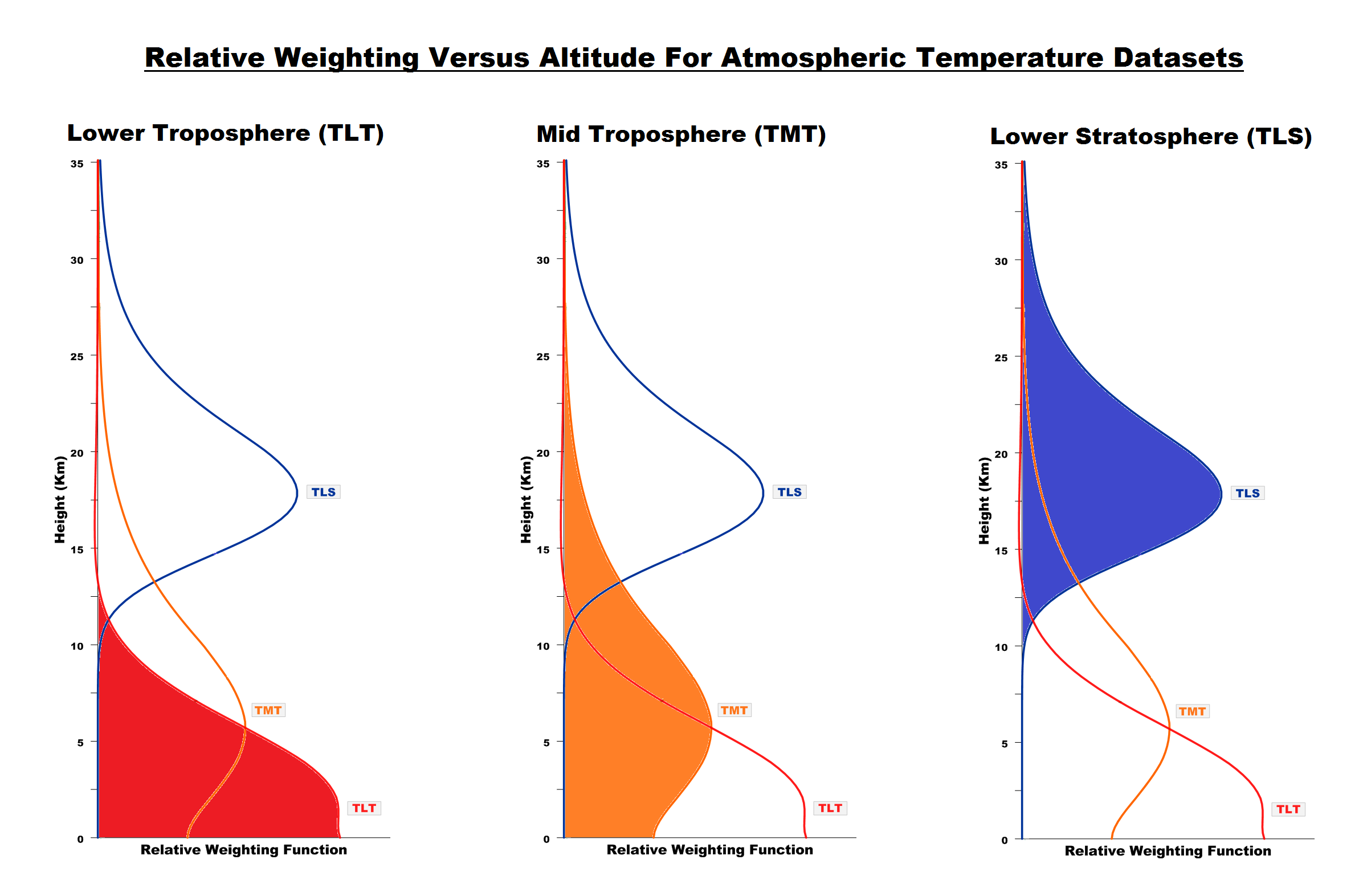
Update: The September 2014 UAH lower troposphere temperature anomaly is +0.30 deg C. It rose (an increase of about +0.10 deg C) since August 2014.

Figure 4 – UAH Lower Troposphere Temperature (TLT) Anomaly Data

RSS LOWER TROPOSPHERE TEMPERATURE ANOMALY DATA (RSS TLT)

Like the UAH lower troposphere temperature data, Remote Sensing Systems (RSS) calculates lower troposphere temperature anomalies from microwave sounding units aboard a series of NOAA satellites. RSS describes their data at the Upper Air Temperature webpage. The RSS data are supported by Mears and Wentz (2009) Construction of the Remote Sensing Systems V3.2 Atmospheric Temperature Records from the MSU and AMSU Microwave Sounders. RSS also presents their lower troposphere temperature data in various subsets. The land+ocean TLT data are here. Curiously, on that webpage, RSS lists the data as extending from 82.5S to 82.5N, while on their Upper Air Temperature webpage linked above, they state:

We do not provide monthly means poleward of 82.5 degrees (or south of 70S for TLT) due to difficulties in merging measurements in these regions.

Also see the RSS MSU & AMSU Time Series Trend Browse Tool. RSS uses the base years of 1979 to 1998 for anomalies.

Update: The September 2014 RSS lower troposphere temperature anomaly is +0.21 deg C. It showed a very slight warming (an increase of about +0.01 deg C) since August 2014.

Figure 5 – RSS Lower Troposphere Temperature (TLT) Anomaly Data

A QUICK NOTE ABOUT THE DIFFERENCE BETWEEN RSS AND UAH TLT DATA

There is a noticeable difference between the RSS and UAH lower troposphere temperature anomaly data. Dr. Roy Spencer discussed this in his September 2011 blog post On the Divergence Between the UAH and RSS Global Temperature Records. In summary, John Christy and Roy Spencer believe the divergence is caused by the use of data from different satellites. UAH has used the NASA Aqua AMSU satellite in recent years, while as Dr. Spencer writes:

…RSS is still using the old NOAA-15 satellite which has a decaying orbit, to which they are then applying a diurnal cycle drift correction based upon a climate model, which does not quite match reality.

I updated the graphs in Roy Spencer’s post in On the Differences and Similarities between Global Surface Temperature and Lower Troposphere Temperature Anomaly Datasets.

While the two lower troposphere temperature datasets are different in recent years, UAH believes their data are correct, and, likewise, RSS believes their TLT data are correct. Does the UAH data have a warming bias in recent years or does the RSS data have cooling bias? Until the two suppliers can account for and agree on the differences, both are available for presentation.

In a more recent blog post, Roy Spencer has advised that the UAH lower troposphere Version 6 will be released soon and that it will reduce the difference between the UAH and RSS data.

13-YEARS+ (165-MONTH) RUNNING TRENDS

As noted in my post Open Letter to the Royal Meteorological Society Regarding Dr. Trenberth’s Article “Has Global Warming Stalled?”, Kevin Trenberth of NCAR presented 10-year period-averaged temperatures in his article for the Royal Meteorological Society. He was attempting to show that the recent halt in global warming since 2001 was not unusual. Kevin Trenberth conveniently overlooked the fact that, based on his selected start year of 2001, the halt at that time had lasted 12+ years, not 10.

The period from January 2001 to September 2014 is now 165-months long—more than 13 years. Refer to the following graph of running 165-month trends from January 1880 to September 2014, using the GISS LOTI global temperature anomaly product.

An explanation of what’s being presented in Figure 6: The last data point in the graph is the linear trend (in deg C per decade) from January 2001 to September 2014. It is basically zero (about +0.02 deg C/Decade). That, of course, indicates global surface temperatures have not warmed to any great extent during the most recent 165-month period. Working back in time, the data point immediately before the last one represents the linear trend for the 165-month period of December 2000 to August 2014, and the data point before it shows the trend in deg C per decade for November 2000 to July 2014, and so on.

Figure 6 – 165-Month Linear Trends

The highest recent rate of warming based on its linear trend occurred during the 165-month period that ended about 2004, but warming trends have dropped drastically since then. There was a similar drop in the 1940s, and as you’ll recall, global surface temperatures remained relatively flat from the mid-1940s to the mid-1970s. Also note that the mid-1970s was the last time there had been a 161-month period without global warming—before recently.

17-YEARS+ (208-Month) RUNNING TRENDS

In his RMS article, Kevin Trenberth also conveniently overlooked the fact that the discussions about the warming halt are now for a time period of about 16 years, not 10 years—ever since David Rose’s DailyMail article titled “Global warming stopped 16 years ago, reveals Met Office report quietly released… and here is the chart to prove it”. In my response to Trenberth’s article, I updated David Rose’s graph, noting that surface temperatures in April 2013 were basically the same as they were in September 1997. We’ll use September 1997 as the start month for the running 17-year trends. The period is now 208-months long. The following graph is similar to the one above, except that it’s presenting running trends for 208-month periods.

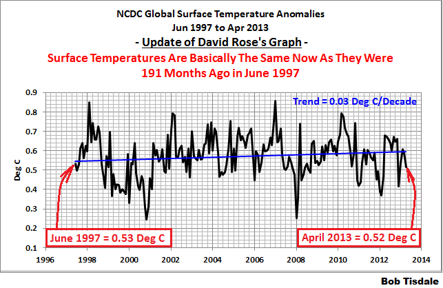
Figure 7 – 208-Month Linear Trends

The last time global surface temperatures warmed at this low a rate for a 208-month period was the late 1970s, or about 1980. Also note that the sharp decline is similar to the drop in the 1940s, and, again, as you’ll recall, global surface temperatures remained relatively flat from the mid-1940s to the mid-1970s.

The most widely used metric of global warming—global surface temperatures—indicates that the rate of global warming has slowed drastically and that the duration of the halt in global warming is unusual during a period when global surface temperatures are allegedly being warmed from the hypothetical impacts of manmade greenhouse gases.

COMPARISONS

The GISS, HADCRUT4 and NCDC global surface temperature anomalies and the RSS and UAH lower troposphere temperature anomalies are compared in the next three time-series graphs. Figure 8 compares the five global temperature anomaly products starting in 1979. Again, due to the timing of this post, the HADCRUT4 and NCDC data lag the UAH, RSS and GISS products by a month. The graph also includes the linear trends. Because the three surface temperature datasets share common source data, (GISS and NCDC also use the same sea surface temperature data) it should come as no surprise that they are so similar. For those wanting a closer look at the more recent wiggles and trends, Figure 9 starts in 1998, which was the start year used by von Storch et al (2013) Can climate models explain the recent stagnation in global warming? They, of course, found that the CMIP3 (IPCC AR4) and CMIP5 (IPCC AR5) models could NOT explain the recent halt in warming.

Figure 10 starts in 2001, which was the year Kevin Trenberth chose for the start of the warming halt in his RMS article Has Global Warming Stalled?

Because the suppliers all use different base years for calculating anomalies, I’ve referenced them to a common 30-year period: 1981 to 2010. Referring to their discussion under FAQ 9 here, according to NOAA:

This period is used in order to comply with a recommended World Meteorological Organization (WMO) Policy, which suggests using the latest decade for the 30-year average.

Figure 8 – Comparison Starting in 1979

###########

Figure 9 – Comparison Starting in 1998

###########

Figure 10 – Comparison Starting in 2001

For those who want to get a rough idea of the impacts of the adjustments to the GISS and HADCRUT4 warming rates, refer to the July update—a month before those adjustments took effect.

AVERAGE

Figure 11 presents the average of the GISS, HADCRUT and NCDC land plus sea surface temperature anomaly products and the average of the RSS and UAH lower troposphere temperature data. Again because the HADCRUT4 and NCDC data lag one month in this update, the most current average only includes the GISS product.

Figure 11 – Average of Global Land+Sea Surface Temperature Anomaly Products

The flatness of the data since 2001 is very obvious, as is the fact that surface temperatures have rarely risen above those created by the 1997/98 El Niño in the surface temperature data. There is a very simple reason for this: the 1997/98 El Niño released enough sunlight-created warm water from beneath the surface of the tropical Pacific to permanently raise the temperature of about 66% of the surface of the global oceans by almost 0.2 deg C. Sea surface temperatures for that portion of the global oceans remained relatively flat until the El Niño of 2009/10, when the surface temperatures of the portion of the global oceans shifted slightly higher again. Prior to that, it was the 1986/87/88 El Niño that caused surface temperatures to shift upwards. If these naturally occurring upward shifts in surface temperatures are new to you, please see the illustrated essay “The Manmade Global Warming Challenge” (42mb) for an introduction.

MONTHLY SEA SURFACE TEMPERATURE UPDATE

The most recent sea surface temperature update can be found here. The satellite-enhanced sea surface temperature data (Reynolds OI.2) are presented in global, hemispheric and ocean-basin bases. We discussed the recent record-high global sea surface temperatures and the reasons for them in the post On The Recent Record-High Global Sea Surface Temperatures – The Wheres and Whys.