EPA document supports ~3% of atmospheric carbon dioxide is attributable to human sources

NOTE: this post has an error, see update below. – Anthony

From a Wry Heat reprinted with permission of Jonathan DuHamel

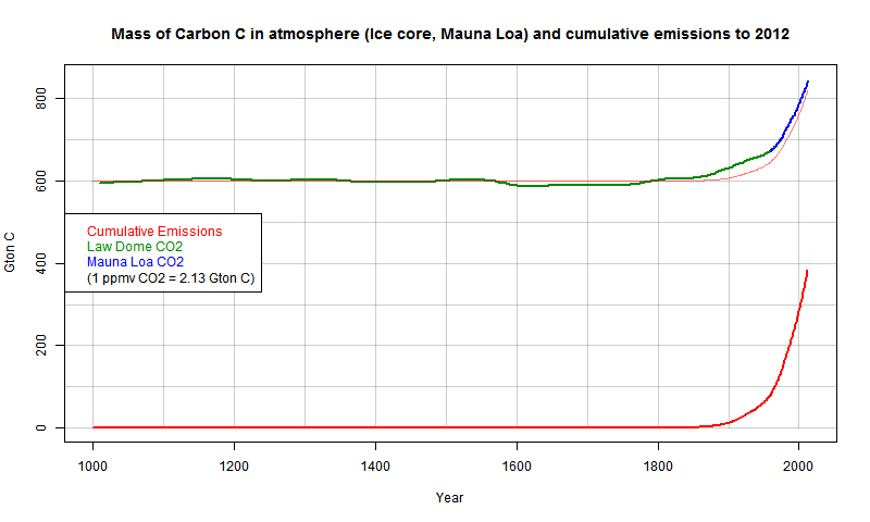
A new post on The Hockey Schtick reviews a new paper “that finds only about 3.75% [15 ppm] of the CO2 in the lower atmosphere is man-made from the burning of fossil fuels, and thus, the vast remainder of the 400 ppm atmospheric CO2 is from land-use changes and natural sources such as ocean outgassing and plant respiration.”

This new work supports an old table from the Energy Information Administration which shows the same thing: only about 3% of atmospheric carbon dioxide is attributable to human sources. The numbers are from IPCC data.

Look at the table and do the arithmetic: 23,100/793,100 = 0.029.

URL for table: http://www.eia.doe.gov/oiaf/1605/archive/gg04rpt/pdf/tbl3.pdf

If one wanted to make fun of the alleged consensus of “climate scientists”, one could say that 97% of carbon dioxide molecules agree that global warming results from natural causes.

===============================================================

UPDATE:

Thanks to everyone who pointed out the difference in the chart and the issues.

I was offered this post by the author in WUWT Tips and Notes, here: http://wattsupwiththat.com/tips-and-notes/#comment-1696307 and reproduced below.

The chart refers to the annual increase in CO2, not the total amount. So it is misleading.

Since the original author had worked for the Tucson Citizen I made the mistake of assuming it was properly vetted.

The fault is mine for not checking further. But as “pokerguy” notes, it won’t disappear. Mistakes are just as valuable for learning. – Anthony Watts

wryheat2 says:

July 28, 2014 at 12:28 pm

Mr. Watts,

John Droz suggested I contact you.

On my blog, I commented on the reasearch by Denica Bozhinova on CO2 content due to fossil fuel burining. She apparently scared The Hockey Schtick into taking down his post on the matter. However, there is an older table from EIA which I reproduce on my post.

Denica Bozhinova has commented extensively, and frankly, I can’t understand her position since she seems to contradict what she wrote in the abstract to “Simulating the integrated summertime Ä14CO2 signature from anthropogenic emissions over Western Europe”

See my post here (you may reprint it if you wish):

http://wryheat.wordpress.com/2014/07/19/only-about-3-of-co2-in-atmosphere-due-to-burning-fossil-fuels/

Jonathan DuHamel

Tucson, AZ

2 4 votes

Article Rating

311 Comments

Inline Feedbacks

View all comments

Ferdinand Engelbeen

July 31, 2014 12:44 am

Bart says:
July 31, 2014 at 12:19 am
That is completely unphysical. They are completely accounted for by the temperature relationship, and you cannot “disconnect” those components of the temperature impetus without some physical mechanism, and that physical mechanism has to high pass “filter” the low frequency components of the temperature variation out and – this is the impossible part – leave no trace of phase distortion in doing so.
Bart, it is proven from the δ13C – CO2 rate of changes match that almost all of the short term variability is from (tropical) vegetation. It is proven from the oxygen balance that vegetation is an increasing net sink for CO2. Thus the short term variability and the long term trend have nothing to do with each other, they are from different processes.
You have no proof at all that the trend is temperature related. If the trend is not temperature related then there is no phase distortion of the short term variability.
In this case there are a lot of indications that the trend is mainly caused by human emissions, thus the observed CO2 rate of change is the sum of temperature caused variability and human caused increase in CO2 rate of change.

Nick Stokes

July 31, 2014 12:48 am

Bart says: July 31, 2014 at 12:23 am
“A superficial, low order polynomial match, with artful graphics to promote a predetermined conclusion.”
There’s no polynomial matching. It’s just ppmv CO2 from Law Dome (CDIAC Etheridge data), Mauna Loa (annual average) and CDIAC emissions data (Boden). 1 ppmv CO2 = 2.13 Gtons C. If you don’t like artful graphics, here is mine.
But yes, it is conclusive.

Bart

July 31, 2014 1:02 am

Ferdinand Engelbeen says:
July 31, 2014 at 12:44 am
” If the trend is not temperature related then there is no phase distortion of the short term variability.”
No. There is a trend in temperature. To remove it, and prevent it from causing a trend in the rate of change of CO2, you would have to filter it out by some exotic process, and that exotic process would have to leave no mark of phase distortion. There is another name for such an exotic process: an impossible process.
Nick Stokes says:
July 31, 2014 at 12:48 am
“There’s no polynomial matching.”
N’enculons pas des mouches. It is inherent in the display. You are looking at two series which have a superficial, low order polynomial type similarity. It is entirely spurious. And, it is diverging.

Nick Stokes

July 31, 2014 1:14 am

Bart says: July 31, 2014 at 1:02 am
“And, it is diverging.”
No, there’s no divergence. Here is the Scripps version of your plot. The match is excellent. It’s not a coincidence.

Bart

July 31, 2014 1:23 am

Nick Stokes says:
July 31, 2014 at 1:14 am
Yes, it is diverging. That is not a “version” of my plot. It is an integration of my plot. It obscures the fact that the emissions are rising super-linearly, while atmospheric concentration is rising only linearly, but you can still make it out if you look closely at the past decade plus, i.e., over the time interval in which global temperatures have stalled.
Come on, Nick. You’re not this stupid. You know perfectly well that all the information in the integral in contained in its derivative, modulo the integration constant. Look at my plot again. The divergence is stark here, when it is on a scale where you can make it out. Stop trying to obfuscate, and deal with what the data are telling us.

tonyb

Editor

July 31, 2014 1:35 am

Alan Robertson said;
‘Wow! That’s quite a response, Ms. Bozhinova. Welcome to WUWT. I hope that you will look favorably on our gracious host’s decision to leave this thread unredacted.”
I endorse that comment. It is good to see the author come over to clarify the content, although as she would have noted the problems were picked up very quickly and noted by our host.
Leaving the thread in place has generated some useful discussion. As someone else mentioned it has been a little while since we have been entertained so royally by Richard and Ferdinand.
I hope Ms. Bozhinova.will come over again or even consider submitting an article here?
tonyb

Nick Stokes

July 31, 2014 1:43 am

Bart says: July 31, 2014 at 1:23 am
“Look at my plot again. The divergence is stark here, when it is on a scale where you can make it out.”
The “divergence” is basically a scale factor. To match the plots, you have to rescale to take account, in effect, of the airborne fraction. Scripps chose 57% (by fitting). You have chosen a factor in which the slope of the blue emissions is greater than the green. It isn’t diverging; it’s not properly matched. This would be more obvious if you deseasonalized the ppmv.

richardscourtney

July 31, 2014 1:51 am

Denica Bozhinova:
I write to support all others who have greeted your arrival here. I draw especial attention to the posts to you from Alan Robertson and the two from davidmhoffer.
Richard

richardscourtney

July 31, 2014 1:53 am

Phil.:
If it makes you happy to think it, then you ‘won’. OK?
Now, be a dear and tidy up your room yourself because I have no intention of going near it.
Richard

Ferdinand Engelbeen

July 31, 2014 2:54 am

Bart says:
July 31, 2014 at 12:23 am
Again distorting the match between emissions and increase in the atmosphere by using different units? Here the real plot with the same units:
http://www.ferdinand-engelbeen.be/klimaat/klim_img/dco2_em4.jpg
increase in the atmosphere as function of human emissions still is largely within natural variability…

Ferdinand Engelbeen

July 31, 2014 3:20 am

Bart says:
July 31, 2014 at 1:02 am
Bart, the short term influence of temperature on CO2 is 4-5 ppmv/°C
The historical influence from decades to multi-millennia is 8 ppmv/°C
The entire temperature trend since 1959 is 0.6°C, good for maximum 5 ppmv CO2 increase. That is all. Hardly visible in the 80 ppmv increase over the same time frame.
Or if you want it in the derivative: no trend in the derivative and only a small offset of 0.1 ppmv/year above zero, hardly influencing the natural, temperature caused year by year variability of +/- 2 ppmv.
As your “match” between temperature and the trend of the CO2 derivative is entirely spurious, either you have to distort the amplitude of the variability, or you have no match between the slopes. The two processes have nothing to do with each other, but you combine them with the same factor.

Samuel C Cogar

July 31, 2014 3:55 am

Alan Robertson says:
July 30, 2014 at 11:42 am
“Hello Mr. Cogar,
Yet, with your response, you didn’t say one single thing to contradict my statement that the planet’s biosphere is greening and biomass increasing. ”
————-
Alan R, there was no reason for me to contradict that part of your statement concerning “greening n’ increasing”.
I disagreed with the “indicates” part of this part of your statement, to wit:
“…. which indicates that annual CO2 bio- uptake outpaces CO2 release from the biosphere.”
——————-
Alan R, just because they have determined there has been an increase in biosphere “greening” due to the “warming” of the climate and the subsequent annual increase in atmospheric CO2 ….. does not prove, infer, suggest or indicate that ….. biomass absorption of CO2 outpaces biosphere emissions CO2 .
If the climate warms, …… then the “growing season” greening is extended in the northern latitudes, …. the microbial ingesting of dead biomass increases, …. permafrost melting increases, …. microbial ingesting of the thawed-out dead biomass increases ….. and the average temperature of the water in the ocean and large lakes increases, …… with all-the-above except for the “greening” emitting CO2 into the atmosphere.
Alan R, if you look at this Keeling Curve graph, http://i1019.photobucket.com/albums/af315/SamC_40/keelingcurve.gif
…. and specifically at that average 6 ppm bi-yearly cycling (sawtooth) of atmospheric CO2, that is, IMLO, ….. the seasonal “heartbeat” of the world’s ocean waters.

Ferdinand Engelbeen

July 31, 2014 5:08 am

Samuel C Cogar says:
July 31, 2014 at 3:55 am
Samuel, we have been there before:
The decay of recent organics can’t outpace the uptake by plants over a longer period of time, simply because the decay would get out of fuel.
All decay, plant use as food or feed, burning of wood etc. only can emit what is already was sequestered in the months to decades before. Thus temporarily you can have a disequilibrium between the two, but over longer runs, that will go at the cost – or benefit – of total vegetation.
Before 1990, the biosphere was near neutral to a small emitter of CO2. After 1990 it became a net increasing sink for CO2, thus more uptake than decay.
and specifically at that average 6 ppm bi-yearly cycling (sawtooth) of atmospheric CO2, that is, IMLO, ….. the seasonal “heartbeat” of the world’s ocean waters.
No, it is the heartbeat of the NH forests: if it were the oceans, the δ13C and CO2 levels would go up and down together. If the biosphere is responsible, δ13C and CO2 levels will go up and down in opposite ways, which is the case here:
http://www.ferdinand-engelbeen.be/klimaat/klim_img/seasonal_CO2_d13C_MLO_BRW.jpg

Samuel C Cogar

July 31, 2014 5:09 am

Ferdinand Engelbeen says:
July 30, 2014 at 1:34 pm
“I have no problems with the unknowns, because the only solution needed is -2, which is all what counts for the increase or decrease of CO2 in the atmosphere.
No matter if X = 150 and Y = 152 or X = 300 and Y = 302”
—————–
Your employment of “fuzzy reverse-mathematics” ….. is highly unProfessional, to say the least.
================
Ferdinand Engelbeen says:
July 30, 2014 at 1:48 pm
“I was talking about the year by year <I<variability of the human emissions. Human emissions indeed are increasing, but the year by year variability and the increase rate from one year to next year is maximum 0.2 ppmv.”
—————-
Ferdinand, “weazelwording” rhetoric doesn’t impress me either.
The sole reason that you are referring to human emissions of CO2 as being a “variability” …… is that you don’t have a frigging clue as to what the actual quantity of those emissions are.
In fact, me thinks you used “reverse mathematics” to guesstimate your “max 0.2 ppmv” figure.

Denica Bozhinova

July 31, 2014 5:43 am

Thank you for the welcome and I apologize if I was a bit harsh in my previous reply. I also do not claim that the pool & pipe analogy is perfect model of the system – it was supposed to be an example of why not only the gross in/outflow are important but also the net contribution of each source.
Another thought, which I did not really see so far brought up in the current discussion – when dealing with idealized box models of the carbon cycle sometimes people forget that the different sources and sinks are actually located in different places over the globe. The ocean will emit and absorb CO2 that is located over the ocean – which means it will absorb mostly CO2 that is already there, or one that requires time to be transported through the atmosphere to those locations. The anthropogenic emissions are located mostly over land in industrialized or highly populated areas, while the big sinks in the biosphere are located in rural areas or in the tropics. It takes time for the anthropogenic CO2 to travel to the places of the biggest natural assimilation. By the time they get there, usually the recently added anthropogenic fraction is well mixed into the atmosphere and it is only a small addition to the recurring biospheric respiration/uptake happening there.

Bart

July 31, 2014 5:53 am

Nick Stokes says:
July 31, 2014 at 1:43 am
“To match the plots, you have to…”
Epicycles.
You are grasping at straws. Why go to such contortions when it is completely unnecessary? This fits, in both the short term and the long, without having to resort to handwaving.

Joe Born

July 31, 2014 5:53 am

Denica Bozhinova: “It takes time for the anthropogenic CO2 to travel to the places of the biggest natural assimilation. By the time they get there, usually the recently added anthropogenic fraction is well mixed into the atmosphere and it is only a small addition to the recurring biospheric respiration/uptake happening there.”
I’ve occasionally wondered whether the locally high concentrations unmeasured by the usual CO2 sensing does not also cause some locally high uptake of some sort that helps explain why half the estimated emissions seem to go unaccounted for. (No doubt this fancy has been thoroughly quashed elsewhere on this site, but I’ve either missed or forgotten it.)

Bart

July 31, 2014 5:57 am

Ferdinand Engelbeen says:
July 31, 2014 at 2:54 am
“Again distorting the match between emissions and increase in the atmosphere by using different units?”
I do not know why this confuses you so. The units has nothing to do with it. My fit is to the first half of the data, to see if it remains true, which it doesn’t. You fit the whole thing, so of course you get a superficial match. You are purposefully fooling yourself.
But, your plot still diverges, with different slopes toward the end of the record.
Ferdinand Engelbeen says:
July 31, 2014 at 3:20 am
“… the short term influence of temperature on CO2 is 4-5 ppmv/°C…”
No, it isn’t. It is very clear that the historical sensitivity in the modern era since 1958 is in units of ppmv/C/unit-of-time. It is an integral relationship. That is an empirical fact.
You are trying to force your model on the data, instead of the data on the model. That is a complete inversion of the scientific method.
“As your “match” between temperature and the trend of the CO2 derivative is entirely spurious, either you have to distort the amplitude of the variability, or you have no match between the slopes.”
It’s a plemty good fit, astoundingly good for the quality of the data, and the bulk measurements involved. You a trying to enforce a completely arbitrary standard.
“The two processes have nothing to do with each other, but you combine them with the same factor.”
Quite the contrary, the fact that you can match both components with the same scale factor is compelling evidence that a temperature dependent process is what is in the driver’s seat.

Ferdinand Engelbeen

July 31, 2014 6:04 am

Samuel C Cogar says:
July 31, 2014 at 5:09 am
Samuel, I did do my best to explain why I think that human emissions are to blame for the recent increase of CO2 in the atmosphere. If you don’t like my explanations, please say where I am wrong, based on observations.
As far as I know, human emissions are quite well known, based on quantities sold by refineries, coal mines and gas exploration firms. If anything, they can be underestimated, not overestimated. Thus worst case, humans emit more than twice the observed increase in the atmosphere.
You may not like my math – which I learned over 55 years ago, but for the C balance it is completely unimportant what the different fluxes are doing during the year. What is important is what the result is at the end of the year: increase, decrease or even. That is what changes the CO2 content of the atmosphere. Not any individual in or out flux.
Thus the only point needed in the whole C balance is the -2 ppmv +/- 1 ppmv/year difference between human emissions and increase in the atmosphere.
is that you don’t have a frigging clue as to what the actual quantity of those emissions are
The year by year emissions inventory can be downloaded from:
http://cdiac.ornl.gov/trends/emis/tre_glob.html up to 2008
and
http://cdiac.ornl.gov/GCP/carbonbudget/2013/ for references to more recent years
If you look at the year by year variability, that is less than 0.2 ppmv.
The lack of variability of the human emissions is important, because some people think that human emissions are not responsible for the increase in the atmosphere as there is no detectable (smaller than 0.1 ppmv) human variability in the rate of change of CO2 in the atmosphere, only a relative huge (+/- 1 ppmv) natural variability.

Samuel C Cogar

July 31, 2014 6:20 am

Janice Moore says:
July 30, 2014 at 10:10 pm
“While this dryly humorous understatement brings a chuckle to the informed, it may mislead some readers if not clarified.
– {39:40} High CO2 values (per SCIAMACHY satellites), i.e., big CO2 sources, are NOT in industrialized nor highly populated regions; they are in Amazon basin, tropical Africa, and SE Asia.”
——————–
Clarification of the above would be nice, ….. but an explanation would be better, ….. as to why and/or how those satellites determined that some of the “warmest” places on the surface of the earth …… were also the biggest sources of CO2.
If the above said CO2 sources are the result of CO2 emissions from the decomposing dead biomass …. then should not the CO2 absorption by the live biomass be “equal to” the aforesaid emissions …. thus resulting in a “net 0 (zero)” CO2 increase in the upper atmosphere?

Ferdinand Engelbeen

July 31, 2014 6:43 am

Bart says:
July 31, 2014 at 5:57 am
I do not know why this confuses you so.
Bart, it seems quite difficult to convince you that you fool yourself:
In your plot the emissions are in Mt/year of CO2. The rise of CO2 is plotted in ppmv/month. If you convert the Mt/year into ppmv/month (factor 1/2120/12) and plot them again, you have the real comparison as I have plotted with the same units: human emissions still about twice the increase in the atmosphere (here in ppmv/year with 12-month running mean for CO2 rate of change):
http://www.ferdinand-engelbeen.be/klimaat/klim_img/dco2_em4.jpg
Your plot gives a false impression of decreasing airborne fraction because you used different units.
No, it isn’t. It is very clear that the historical sensitivity in the modern era since 1958 is in units of ppmv/C/unit-of-time. It is an integral relationship. That is an empirical fact.
No, that is whole point of the discussion: there never is or was a sensitivity as ppmv/°C/unit of time. There always was a clear sensitivity of 4 to maximum 8 ppmv/°C independent of time or lag. The latter even over thousands of years between glacials and interglacials and back. Your integration is only based on the good match between T (again, in fact dT/dt) variability and dCO2/dt variability, while the slope of dCO2/dt has nothing to do with T. The variability of dCO2/dt is caused by dT/dt, with a pi/2 lag, not by T. If you integrate dT/dt that will give maximum 5 ppmv CO2 over the past period and the full variability of dCO2/dt:
http://www.ferdinand-engelbeen.be/klimaat/klim_img/temp_dco2_d13C_mlo.jpg
the fact that you can match both components with the same scale factor is compelling evidence that a temperature dependent process is what is in the driver’s seat.
The proven fact that slope and variability are from different processes confirms that the “match” is entirely spurious. If the slope changes you need to adjust the matching factor which also changes the amplitude of the variability, while amplitude and slope have nothing to do with each other.

Alan Robertson

July 31, 2014 6:44 am

Samuel C Cogar says:
July 31, 2014 at 3:55 am
“Alan R, just because they have determined there has been an increase in biosphere “greening” due to the “warming” of the climate and the subsequent annual increase in atmospheric CO2 ….. does not prove, infer, suggest or indicate that ….. biomass absorption of CO2 outpaces biosphere emissions CO2 .”
______________________
Topsoil.

Samuel C Cogar

July 31, 2014 7:53 am

Ferdinand Engelbeen says:
July 31, 2014 at 6:04 am
“Samuel, I did do my best to explain why I think that human emissions are to blame for the recent increase of CO2 in the atmosphere.”
—————
Ferdinand, I know you did your best., …. but oftentimes one’s best is not the “bestest” best.
And iffen that was not a “truism” …. then there would never be a need to obtain the services of a consultant.
================
“If you don’t like my explanations, please say where I am wrong, based on observations.”
—————-
Ferdinand, that is easy enough for me to do ….. just by “observing” your next comment, to wit:
==============
“As far as I know, human emissions are quite well known, based on quantities sold by refineries, coal mines and gas exploration firms. If anything, they can be underestimated, not overestimated.”
——————
Ferdinand, your above said “As far as I know” …. and …. “are quite well known” …. is/are equivalent to a “consensus of opinion(s)” ….. and therefore has no basis in supporting proof or evidence of actual, factual science.
And secondly, to first state that … “quantities sold are quite well known” …. and then assert that the aforesaid “quantities sold” ….. could very well be UNDERESTIMATED, … but surely not OVERESTIMATED, …… is asinine, silly and/or idiotic.
Well known estimations ….. is a dog that won’t hunt.
That is, unless you are playing “Sciency Horseshoes” …. where anything that is reasonably close or not too far way …. “counts” as an honest-to-goodness “fact of science”.
Ferdinand, in all of the above postings there are very few actual, factual “numerical” quantities being discussed. And if one is not employing actual, factual “numerical” quantities in their calculations ….. then they should not be claiming, inferring or asserting that the results of their calculations are factual evidence or proof of anything.
“Averages” are NOT actual “numerical” quantities of anything. They are abstract “numbers” that represent the mean or medium value of a specific number “set” or group of numbers and should only be used as “reference” information of or about a “past” event.

Ferdinand Engelbeen

July 31, 2014 8:24 am

Samuel C Cogar says:
July 31, 2014 at 7:53 am
It is not because I am expressing my thoughts in a civil manner, that they are mere opinions…
There are inventories of fossil fuel use and its CO2 emissions. That is a fact.
They may be underestimated not overestimated. That is an opinion, based on the human nature to avoid taxes.
The inventories thus are the absolute minimum of the human emissions. That is a fact.
That minimum is larger than what is measured as increase in the atmosphere. That is a fact.
The difference between increase in the atmosphere and human emissions is what nature absorbs. That is a fact.
At minimum nature was a continuous and increasing sink for CO2 over the past 55 years. That is a fact.
Thus the net contribution of nature to the increase of CO2 in the atmosphere was?

Samuel C Cogar

July 31, 2014 8:42 am

Ferdinand Engelbeen says:
July 31, 2014 at 5:08 am
“Samuel, we have been there before:
No, it is the heartbeat of the NH forests: if it were the oceans, the δ13C and CO2 levels would go up and down together. If the biosphere is responsible, δ13C and CO2 levels will go up and down in opposite ways, which is the case here:”
—————–
“YES”, we have.
But you went “POOF”, like the Magic Dagon and did not respond to my post discrediting your unsupported “tripe n’ piffle” …. which I posted on January 14, 2014 at 10:01 am at this url link address, to wit:
http://wattsupwiththat.com/2014/01/09/now-its-the-fungi-carbon-footprint-that-isnt-in-climate-models/#comment-1535697
Ferdinand, “running n’ hiding” doesn’t prove you are correct.