Guest essay by Joe Born
In a recent post Christopher Monckton identified me as a proponent of the following proposition: The observed decay of bomb-generated atmospheric-carbon-14 concentration does not tell us how fast elevated atmospheric carbon-dioxide levels would subside if we discontinued the elevated emissions that are causing them. He was entirely justified in doing so; I had gone out of my way to bring that argument to his attention.
But I was merely passing along an argument to which a previous WUWT post had alerted me, and the truth is that I’m not at all sure what the answer is. Moreover, semantic issues diverted the ensuing discussion from what Lord Monckton probably intended to elicit. So, at least in my view, we failed to join issue.
In this post I will attempt to remedy that failure by explaining the weakness that afflicts the position attributed (again, understandably) to me. I hasten to add that I don’t profess to have the answer, so be forewarned that no conclusion lies at the end of this post. But I do hope to make clearer where at least this layman thinks the real questions lie.

To start off, let’s review the argument I made, which is that the atmospheric-carbon-dioxide turnover time is what determined how long the post-bomb-test excess-carbon-14 level took to decay. That argument was based on the “bathtub” model, which Fig. 1 depicts. The rate at which the quantity <i>m</i> of water the tub contains changes is equal to the difference between the respective rates <i>e</i> (emissions) and <i>u</i> (uptake) at which water enters from a faucet and leaves through a drain:

The same thing can, <i>mutatis mutandis</i>, be said of contaminants (read carbon-14) in the water. But in the case of well-mixed contaminants one of the <i>mutanda</i> is that the rate at which the contaminants leave is dictated by the rate at which water leaves:

where 

Consequently, if the water quantity increases for an interval during which <i>e</i> exceeds <i>u</i>, it will thereafter remain elevated if the emissions rate <i>e</i> then falls no lower than the drain rate <i>u</i>. If a dose of contaminants is added to the water, though, the resultant contaminant amount falls, even when there’s no difference between <i>u</i> and <i>e</i>, in accordance with the <i>turnover</i> rate, i.e., with the ratio of <i>u</i> to <i>m</i>. So, to the extent that this model reflects reality’s relevant aspects, we can conclude that the rate at which the carbon-14 concentration decays tells us nothing about what happens when total-CO2 emissions return to a “normal” level.
But among the foregoing model’s deficiencies is that it says nothing about a possible dependence of overall drain rate <i>u</i> on the water quantity <i>m</i>, whereas we may expect biosphere uptake (and emissions) to respond to the atmosphere’s carbon-dioxide content. Nor does it deal with the possibility that after contamination has flowed out the drain it will be recycled through the faucet. In contrast, the biosphere no doubt returns to the atmosphere at least some of the carbon-14 it has previously taken from it.

A model that takes such factors into account could support a conclusion different from the one to which the bathtub led us. Consistently with my last post’s approach, Fig. 2 uses interconnected pressure vessels to represent one such model. In this case there are only two vessels, the left one representing the atmosphere and the right one representing carbon sinks such as the ocean and the biosphere.
The vessels contain respective quantities 


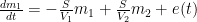
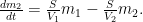
Those equations tell us that the carbon quantity 
![m_1(t) = \left[ \frac{V_1}{V_1+V_2}+\frac{V_2}{V_1+V_2} \exp\left(-\frac{V_1+V_2}{V_1V_2}St \right)\right] m_0 ,](https://s0.wp.com/latex.php?latex=m_1%28t%29+%3D+%5Cleft%5B+%5Cfrac%7BV_1%7D%7BV_1%2BV_2%7D%2B%5Cfrac%7BV_2%7D%7BV_1%2BV_2%7D+%5Cexp%5Cleft%28-%5Cfrac%7BV_1%2BV_2%7D%7BV_1V_2%7DSt+%5Cright%29%5Cright%5D+m_0+%2C+&bg=ffffff&fg=000&s=0&c=20201002)
which the substitutions 

Note that in the Fig. 2 system any constituent of the gas would be exchanged between vessels in accordance with the partial-pressure difference of that constituent alone, as if it were the only component the vessels contained. By thus constraining the flow from (and to) the first, atmosphere-representing vessel, this model supports the conclusion that the overall-carbon-dioxide quantity would, contrary to my previous argument, decay just as the excess, bomb-caused quantity of atmospheric carbon-14 did.

Could providing more than one sink enable us to escape that conclusion? Not necessarily. Consider the more-complex system that Fig. 3 depicts. Just as the system that my previous post described, this one can embody the TAR Bern-model parameters. As that post indicated, describing such a system requires a fourth-order linear differential equation. So that system does have more degrees of freedom in its initial conditions and can therefore exhibit a wider range of responses.
But it still constrains the flow among its four vessels linearly in accordance with partial pressures, just as the Fig. 2 system does. From complete equilibrium, therefore, its behavior for any constituent is the same as for any other constituent as well as for the contents as a whole. In other words, this model, too, seems to support the notion that the bomb-test results do indeed tell us how long excess carbon dioxide will remain if we stop taking advantage of fossil fuels.
In a sense, though, the models of Figs. 2 and 3 beg the question; they use the same uptake- and emissions-process-representing
So one question is how significant that difference is in the present context. I don’t have the answer, although my guess is, not very. But readers attempting to answer that question could do worse than start by referring to a previous WUWT post by Ferdinand Engelbeen.

Another way in which carbon-14 differs from the other two carbon isotopes is that it’s unstable. So, if the Fig. 3 model is adequate for carbon-12 or -13, a different model, which Fig. 4 depicts, would have to be used for carbon-14 if its radioactive decay is significant. That diagram differs from Fig. 3 in that it includes a flow 
To the extent that those different models produce different responses, using bomb-test data to predict the total carbon content’s behavior is problematic. But the Engelbeen post mentioned above seems to say that even deep-ocean residence times tend to be only a minor fraction of carbon-14’s half-life: this factor’s impact may be small.
A possibly more-significant factor is that the carbon cycle is undoubtedly non-linear, whereas the conclusions we tentatively drew from the models above depend greatly on their linearity. Before I reach that issue, though, I should point out an aspect of the Bern model that was not relevant to my previous post. The Bern equations I set forth in my last post were indeed linear. But that does not mean that their authors meant to say that the carbon cycle itself is. Although for the sake of simplicity I’ve discussed the models’ physical quantities as though they represented, e.g., the entire mass of carbon in a reservoir, their authors no doubt intended their (linear) models’ quantities to represent only the differences from some base, pre-industrial values. Presumably the purpose was to limit their range enough that the corresponding real-world behavior would approximate linearity.
But such linearization compromises the conclusions to which the models of Figs. 2 and 3 led us. A linear system is distinguished by the fact that its response to a composite stimulus always equals the sum of its individual responses to the stimulus’s various constituents; if the stimulus equals the sum of a step and a sine wave, for example, the system’s response to that stimulus will equal the sum of what its respective responses would have been to separate applications of the step and the sine wave. And this “superposition” property was central to drawing the conclusions we did from those models: the response to a large stimulus is proportionately the same as the response to a small one.

To appreciate this, consider Fig. 5, which depicts scaled values of the Fig. 2 model’s left-vessel total-carbon and carbon-14 contents. Initially, the system is at equilibrium, with zero outside emissions 


At time t = 5, a bolus of carbon-14 appears in the (atmosphere-representing) left vessel. Compared with the total carbon content, the added quantity is tiny, but it is large enough to double the small existing carbon-14 content. As the distance between the red dotted vertical lines shows, the resultant increase in carbon-14 content decays toward its new equilibrium value with a time constant of just about seven years. (I’ve assumed that the processes greatly favor the sink-representing right vessel—i.e., that its “volume” is much greater than the left vessel’s—so that the new equilibrium value is not much greater than the original.)
Now consider what happens at t = 45, when the left vessel’s total-carbon quantity suddenly increases. Although the two quantities are scaled to their respective initial values, this total-carbon increase is orders of magnitude greater than the t = 5 carbon-14 increase. Yet, as the black dotted vertical lines show, the decay of the left vessel’s total-carbon content proceeds just as fast proportionately as the much-smaller carbon-14 content did. As was observed above, this could tempt one to conclude that the carbon-14 decay we’ve observed in the real world tells us how fast the atmosphere would respond to our discontinuing fossil-fuel use.
![clip_image009[1]](http://wattsupwiththat.files.wordpress.com/2013/12/clip_image0091.png?quality=75 "clip_image009[1]")
But now consider what can happen if we relax the linearity assumption. Specifically, let’s say that the Fig. 2 model’s proportionality “constant”

In that plot, the red lines show that the carbon-14 decay occurs just as fast as in the previous plot, the carbon-14 content falling to exp(-1) above its new equilibrium value in around seven years. But the much-larger total-carbon increase brings the system into a lower-efficiency range, so that quantity subsides at a more-leisurely pace, taking over forty years. If such results are any indication, bomb-test results are a poor predictor of how long total-carbon content will settle.
Now permit me a digression in which I attempt to forestall pointless discussion of precisely what the quantities are that the graphs show. I believe the exposition is clearest if it is directed, as in Figs. 5 and 6, to ratios that carbon 14 and total carbon bear to their own initial values. But it appears customary to express the carbon-14 content instead in terms of its ratio to total carbon content. This means that, since total carbon has been increasing, the numbers commonly used in carbon-14 discussions could fall below the pre-bomb values, even though total carbon-14 has in fact increased.
For the sake of those to whom that issue looms large, I have attached Fig. 7 to illustrate how the values for carbon-14 itself could differ from those of its ratio to total carbon in a situation in which new (carbon-14-depleted) carbon is continually injected into the atmosphere.

But that’s a detail. More important is the issue that Fig. 6 raises.
Now, I “cooked” Fig. 6’s numbers to emphasize the point that nonlinearity can undermine conclusions based on linear models. Specifically, Fig. 6 depicts the results of making the flows proportional only to the fifth root of the carbon content.
But non-linearity must have some effect. How much? I don’t know. Together with the differences in behavior between carbon-14 and its stable siblings, though, it is among the considerations to take into account in assessing how informative the bomb-test data are.
As I warned at the top of the post, this post draws no conclusions from these considerations. But maybe the foregoing analysis will prompt knowledgeable readers’ comments that help narrow the issues.
DocMartyn says:
December 12, 2013 at 5:38 pm
Doc, if you should read a lot of what is published in the literature, you should know that the main transfer between the atmosphere and the deep oceans and back is mostly via relative small areas which are quite defined, but variable with wind speed and direction (like the El Niño events). The measured transfer rate is highest at the upwelling places around the equator and the downwelling places near the poles:
http://www.pmel.noaa.gov/pubs/outstand/feel2331/images/fig06.jpg
That are calculated values, based on measurements.
Not by coincidence, the main upwelling places are the places with the highest influx (deep oceans to atmosphere) and the main downwelling places are the places with the highest outflux (atmosphere to deep oceans). That are the places where there is a direct connection between the atmosphere and the deep oceans via a massive waterflow. That can be followed by human-made tracers like 14C and CFC’s etc… There is hardly any trace of the 14C bomb spike in the deep oceans, except at the sink places, but there is at the ocean surface. Thus there is hardly any direct carbon exchange between most of the surface layer and the deep oceans.
The decay rate of 14C shows you the residence time of any individual molecule CO2 (all isotopes alike) in the atmosphere. It does NOT show you how fast some extra CO2 mass injection above equilibrium will decay. Simply as both processes are (near) completely independent of each other: you can have a decay of 14CO2 with increasing total CO2 (as we have had in the past decades), decreasing total CO2 and leveled total CO2.
The decay rate of any extra injection of 14C depends of the residence time, which depends of the throughput (in or out of ~800 GtC / 150 GtC/yr) which is ~5 years.
The decay rate of a mass pulse of total CO2 depends of the difference between inputs and outputs, which is a measured 4.5 GtC/yr for a measured 231 GtC above equilibrium or 231/4.5 = ~51 years.
Hoser says:
December 12, 2013 at 6:29 pm
To summarize, there are two conclusions I tentatively come to. 1) Humans cannot be the cause of the rise in CO2 because the rise is much greater than the amount of CO2a that should be present given the simple model and t1/2 of 5 years.
The 5 years is for the exchange rate, which is the decay rate for an isotope pulse (as concentration, not as mass), which has not the slightest connection with the decay rate of a mass pulse in the atmosphere. If you inject 100 GtC “human” CO2 with low carbon into the pre-industrial atmosphere, the “human” CO2 will be replaced by “natural” CO2 within 60 years, while the increase in the atmosphere still is 40% of the initial extra mass. Still caused by the human CO2 injection, while near none of the original human molecules are left in the atmosphere:
http://www.ferdinand-engelbeen.be/klimaat/klim_img/fract_level_pulse.jpg
Where FA the fraction of human CO2 in the atmosphere, FL in the ocean surface layer tCO2 total CO2 and nCO2 natural CO2.
Thus your conclusion is right for following the fate of the human emissions, but wrong about the cause of the increase in the atmosphere, which is near fully from the human emissions…
We tend to skip quickly past the well known observation that living things preferentially select lighter isotopes as if this were a simple effect. I submit we may be well served to hold the high order differential equations a moment and ponder this effect. For starters, how do they do it? We know that it is not a hard filter because heavier isotopes are definitely utilized and incorporated, particularly when the preferred 12CO2 is unavailable.
What makes this effect hard to model is that it seems PURPOSEFUL. 14C is definitely the pariah isotope in the biological cycle so its removal from the atmosphere will be skewed to the inorganic processes. One can imagine this will cut both ways regarding 14C residence in the atmosphere and ocean surface, depending on various rates.
It is also peculiar that 13C is concentrated in the oceans. They seem to be a repository for rejected isotopes. It would be interesting to know the isotopic variation with depth.
Perhaps the purposeful uptake of the 12CO2 we produce and an increase in the biological cycle rate answer Lord Mockton’s question why half of our production disappears instantaneously.
I find all this detailed analysis interesting , but I’m with the group who just took one look at the jaggies in the Mauna Loa data and immediately eyeballed that the half life of CO2 could not be more than a couple of decades and thus claims in terms of centuries or millennia were inexcusable nonscience . Unless there were large nonuniformities in CO2 concentration which happened to cross Mauna Loa seasonally , and it’s been commented here that CO2 is in fact well mixed , the seasonal relaxation must be following a , not surprisingly , substantial seasonal hemispheric variation in production .
Just grabbing the first jaggy in http://wattsupwiththat.com/2008/04/06/co2-monthly-mean-at-mauna-loa-leveling-off/ , I get a variation of about 1.8% in half a year . Since CO2 production is still far from zero even in the Northern Winter , rounding to 0.98 , we find that declines to 0.50 in about 34 cycles , or 17 years . That’s close enough to wonder how any paper claiming half-lives in centuries could be published anywhere rather than be instantly ridiculed to the ash heap even by science journalists .
But given that James Hansen’s claim that Venus is the result of a “runaway greenhouse effect” didn’t get him immediately laughed out of a job on the most basic non-optional radiative balance computations , this is just detail .
Btw ; I find 10 digit numbers when only a couple or three are meaningful too much visual noise to parse .
Bob Armstrong says:
December 13, 2013 at 9:53 am
……. we find that declines to 0.50 in about 34 cycles , or 17 years . That’s close enough to wonder how any paper claiming half-lives in centuries could be published anywhere rather than be instantly ridiculed to the ash heap even by science journalists .
—————————————————————
If you can get a “centuries” number into the “peer-reviewed” literature and out into the AGW-taxation-fraud media, it can get you elected into the National Academy don’t you know ?
I once suggested on here that given that it’s likely that every carbon atom on planet Earth has been in the atmosphere at some point in its history, then the half-life could be measured in billions of years. Still waiting for my prize.
DocMartyn: “The problem we have with polar waters as down welling ‘sinks’ for DIC, based on Henry’s law, is that these polar oceans at the edge of the ice caps are highly bio-productive and the surface is denuded of DIC during the summer months.”
Thank you for your response. What I infer from it is that determining uptake by the deep oceans in the uptake regions should not be based on the difference between the atmospheric partial pressure and the general mixed-layer partial pressure, because in the summer biological activity denies the depths dissolved inorganic carbon. But I’m still toying with the idea of trying out the model whose ocean portion I laid out in that last comment to Mr. Engelbeen, and I’m still thinking I’ll have the winter uptake be proportional to the general mixed-layer partial pressure but have h_u fudge factor reflect not only Henry’s Law but also your just-quoted observation.
gymnosperm: “We tend to skip quickly past the well known observation that living things preferentially select lighter isotopes as if this were a simple effect. I submit we may be well served to hold the high order differential equations a moment and ponder this effect. ”
I plead guilty of that charge, but you may want to consult this http://www.ferdinand-engelbeen.be/klimaat/co2_measurements.html#The_mass_balance page to get at least one person’s (Mr. Engelbeen’s) thoughts on those preferences and then look here http://www.ferdinand-engelbeen.be/klimaat/klim_img/fract_level_pulse.jpg for conclusions he drew.
A reason why I personally haven’t focused on it is that I first want to get a little better understanding of the pathways before I assign them isotope preferences.
As you say, though, I may be putting the cart before the horse.
phlogiston says:
December 13, 2013 at 2:28 am
A radiotracer measures a single removal term. PERIOD. A pulse of CO2 enters the atmosphere different from the other CO2 due to 14C. So it can be tracked in exclusion of any other CO2.
No problem with that at all.
The only real question as to the validity of the bomb 14CO2 loss data is that of the extent and speed of atmospheric mixing at the start. I’m not clear if you were referring to this. But this probably has the potential to modify the 5 year result only a minor way.
There are no problems with the atmospheric mixing, apart of a small delay of a few years between the NH and the SH.
It is an essential prerequisite of an effective kinetic tracer that it is NOT recycled back into the measured compartment. So the fact that bomb 14CO2 is not returned from sea to atmosphere serves only to underpin the validity of this measurement of 5 year t1/2 removal of CO2 from the atmosphere.
No problem with that either. 14CO2 is a very good tracer of the residence time of any CO2 molecule in the atmosphere.
But what seems extremely difficult to understand by some here, while most housewives with a household budget have no problems with that: is is not about how fast your money is coming in and going out of your wallet or how long a 1 euro piece or 1 dollar bill resides in your wallet, it is about how much money is left in your wallet at the end of the day… That are quite different decay rates (be it not for every housewife)…
philincalifornia says:
December 13, 2013 at 5:07 am
I think the resistance to assimilating the actual, real data, such resistance manifesting itself as pages and pages of mental masturbation, is because plugging in that real number for the half-life (probably the most important number of all) destroys the mass balance argument and many other such preconceived conclusion-based arguments.
There is not the slightest resistance to use the 5 years residence time or the 14C decay data by the “warmers”. It is mentioned in the Bern model as “decay rate of an isotopic pulse”, which is much faster than for a CO2 mass pulse. Another use is for checking the ocean circulation models, as mentioned in the short description of the Bern model:
http://www.climate.unibe.ch/~joos/model_description/model_description.html
Myrrh says:
December 13, 2013 at 3:29 am
How can there possibly be any educated description of the Carbon Cycle which eliminates precipitation?
For the simple reason that pecipitation is a very small component in the carbon cycle, largely negligible. Even if the water cycle doubled, it only would transport twice the amounts of carbon in/out the atmosphere within a few days, which completely levels out in yearly averages
Donald L. Klipstein says:
December 12, 2013 at 8:52 pm
My take: With ocean acidification reducing global ocean surface pH from 8.25 to 8.14, and mentions of ocean hydrogen ion content increasing by 26%, I figure that the upper ocean is in equilibrium with atmospheric CO2 content of 353 PPMV.
Careful: you are looking at the ocean surface only. The ocean surface layer follows the atmosphere changes with a very fast rate: 1-2 years. That means that the average pCO2 of the ocean surface is only 7 μatm less than the increasing CO2 levels in the atmosphere. But that is not the equilibrium setpoint, that is only the result of the increase in the atmosphere. See:
http://www.pmel.noaa.gov/pubs/outstand/feel2331/exchange.shtml
While the ocean surface is readily saturated, the deep oceans are far from saturated, but there is only a limited exchange between atmosphere and deep oceans. That makes that the overall decay time is ~50 years for the pre-industrial setpoint of ~290 ppmv for the current temperature.
Ferdinand, do you know where/if the (most recent) high quality 14C data from Jungfraujoch can be found? I have seen a graph of it somewhere, but not with available data.
Ferdinand, you appear to have a large void in understanding.
Fact
1) The dilution of 14CO2 has a t1/2 of 12.5 years.
Fact
2) The dilution is into a kinetically infinite pool; and so this 12.5 years represents the movement of 14CO2 from the atmosphere into the lower depths of the ocean.
Fact
3) 14CO2 is almost chemically identical to 12CO2, and we can therefore assume that in 12.5 years half of the total CO2 in the atmosphere exchanges with the deep ocean.
Fact
4) Prior to the burning of fossil fuels the movement of CO2 into the deep oceans and out of the deep oceans would have been identical.
Fact
5) The burning of fossil fuels injects CO2 into the atmosphere, and so the amount of CO2 in the atmosphere has increased. It follows that the AMOUNT of CO2 being transferred from the atmosphere into the deep ocean will increase in proportion to the elevated atmospheric CO2 fraction.
Fact
6) As the total CO2/DIC reservoir of the deep ocean is huge, we can be sure that the amount of CO2 entering the atmosphere from the deep ocean is unchanged from the pre-industrial amount.
No assertions. No mechanisms. No armwaving.
Which of these statements do you believe to be incorrect?
What kinetic, as opposed to mechanistic, argument have you in refutation?
Joe Born says:
December 13, 2013 at 3:51 am
The rate of CO2 flow from the atmosphere is proportional to the sum of the respective rates , , and at which it flows into the general mixed layer, the uptake (downwelling) region, and the emissions (upwelling) regions. For the sake of simplicity, we’ll consider those three quantities not actually as flow rates but rather as components of partial-pressure change rate.
I suppose that this based on fig.3. That is also what DocMartyn prefers, but you will get into trouble with that scheme:
– There is a lot of exchange between the atmosphere and the ocean surface over the seasons (about 60 GtC in/out), but the net result is a change of 10% of the increase in the atmosphere, due to the buffer (Revelle) factor. Thus an increase of 4.5 GtC/yr (2 ppmv/yr) in the atmosphere is fast (decay time 1-2 years) followed by an increase of 0.45 GtC in the ocean surface (total carbon amounts in the mixed layer and the atmosphere are near equal).
– There is little exchange between the mixed layer and the deep oceans. The 7 GtC/yr from DocMartyn may be right.
– There is a relative huge transfer from the atmosphere directly into the deep at the poles and from the deep into the atmosphere near the equator of about 40 GtC/yr (based on the 13CO2 “dilution” from the human emissions by deep ocean CO2).
Therefore I would connect the deep ocean transfer directly to the atmosphere, as the transfer rate of carbon is slower than for the surface layer, but the carbon flux is a magnitude larger than the carbon flux between the mixed layer and the deep oceans and the net transfer also is a magnitude larger:
Of the ~9 GtC emitted by humans, ~0.5 GtC is absorbed by the mixed layer, ~1 GtC by vegetation and ~3 GtC by the deep oceans.
Then a general remark: the 14C as tracer shows you the decay rate of any isotope pulse in the atmosphere relative to other isotopes, which is throughput dependent, but doesn’t show you the effect of an increase of total CO2 in the atmosphere, which is in/out flux difference dependent.
DocMartyn says:
December 13, 2013 at 12:09 pm
Agreed with 1) and 2) be it that part also is removed by the ocean surface and vegetation, but to a lesser extent.
3) 14CO2 is almost chemically identical to 12CO2, and we can therefore assume that in 12.5 years half of the total CO2 in the atmosphere exchanges with the deep ocean.
That is an interesting one: thus 400 GtC is exchanged with the deep oceans in 12.5 years or a througput of 32 GtC/year. My own estimate of 40 GtC/yr for the exchange rate between atmosphere and deep oceans is not far off…
4) and 5) agreed.
6) As the total CO2/DIC reservoir of the deep ocean is huge, we can be sure that the amount of CO2 entering the atmosphere from the deep ocean is unchanged from the pre-industrial amount.
Wrong: as good as the flux from atmosphere into the deep oceans increases from the increased pCO2 in the atmosphere (and still the same pCO2 in the oceans as before), the flux from the deep oceans into the atmosphere decreases because of the increased pCO2 in the atmosphere (and still the same pCO2 in the oceans as before).
In fact not that important, as the net difference between in- and outfluxes is known, no matter if that is a change in influx or outflux or both.
And you forgot 7).
7) The net measured difference in in/outflux between atmosphere and deep oceans is ~3 GtC/yr. For a 231 GtC increase in the atmosphere above equilibrium that gives an e-fold decay rate for an impulse of an extra CO2 mass in the atmosphere into the deep oceans of 231/3 = 77 years.
The latter is not different if the basic exchange rate between the atmosphere and the deep oceans is 32 GtC/yr or 40 GtC/yr or 400 GtC/yr.
Thus simply said: the 14C bomb concentration spike decay rate shows you the exchange rate between the atmosphere and the deep oceans, but that doesn’t give us any clue what will happen with an excess injection of extra CO2 mass in the atmosphere.
“My own estimate of 40 GtC/yr for the exchange rate between atmosphere and deep oceans is not far off…”
A 12.5 year half-life gives you a rate of 0.056 y-1, so the annual rate is 765 GtC*0.056 = 42 GtC
“the flux from the deep oceans into the atmosphere decreases because of the increased pCO2 in the atmosphere (and still the same pCO2 in the oceans as before)”
So how does a CO2 molecule in the deep ocean know that the atmosphere 1 km above its head has an increase in the amount of CO2, so that it decides not to diffuse upward?Do you send a daily telegram to the carbon in the deep ocean and tell it which direction it should move, because you think it is more entropically viable?
michael hart says:
December 13, 2013 at 11:28 am
Ferdinand, do you know where/if the (most recent) high quality 14C data from Jungfraujoch can be found? I have seen a graph of it somewhere, but not with available data.
Recent data from Jungfraujoch and Schauinsland (2000-2012) at:
http://www.tellusb.net/index.php/tellusb/article/download/20092/pdf_1
14CO2 data (1976-1996) from Schauinsland at CDIAC:
http://cdiac.ornl.gov/trends/co2/contents.htm
Graphs from 1985 on:
http://archiv.ub.uni-heidelberg.de/volltextserver/6745/1/LevinRAD2004.pdf
At last I did find the data:
http://www.iup.uni-heidelberg.de/institut/forschung/groups/kk/Data_html
DocMartyn says:
December 13, 2013 at 1:45 pm
A 12.5 year half-life gives you a rate of 0.056 y-1, so the annual rate is 765 GtC*0.056 = 42 GtC
Stupid me, indeed it is a half life not a ratio…
Well, my estimate was based on the 13C/12C ratio. The 14C/12C ratio gives the same result…
So how does a CO2 molecule in the deep ocean know that the atmosphere 1 km above its head has an increase in the amount of CO2, so that it decides not to diffuse upward?Do you send a daily telegram to the carbon in the deep ocean and tell it which direction it should move, because you think it is more entropically viable?
Forget migration from the deep oceans to the atmosphere and back, or even from deep oceans to the mixed layer and back. There is virtually none. Most of the carbon exchanges is by mechanical means: ocean currents and wind.
The deep ocean – atmosphere exchanges are from downwelling and upwelling waters. The downwelling waters are extremely low in pCO2 thus can take a lot of CO2 with them in the deep, if stirred by wind. The upwelling waters are extremely high in pCO2, thus can release a lot of CO2, if stirred by wind. In both cases it is the pCO2 difference with the atmosphere (+ wind speed) which dictates the resulting fluxes, see:
http://www.pmel.noaa.gov/pubs/outstand/feel2331/maps.shtml
Rainfall in the tropical band within 1000 km of the equator drops about 150,000,000,000 tons of CO2 into the oceans p.a. absorbed into raindrops. This surely affects the rate at which 14C is removed from the atmosphere.
Ferdinand Engelbeen:
–“I suppose that this based on fig.3. That is also what DocMartyn prefers . . . I would connect the deep ocean transfer directly to the atmosphere”
Actually, I’m attempting to implement a hybrid. My intent is for the transfer to be basically direct, as you say, between the deep ocean and the atmosphere. I treat the deep-ocean capacity as essentially infinite, using just a constant P_h for the deep-ocean partial pressure by which its emissions to the atmosphere are calculated. But it didn’t seem quite right for the partial pressure used to calculate deep-ocean uptake to be constant; wouldn’t that be determined by (but less than) the mixed layer’s partial pressure? So I’m largely following what you said: there are uptake and emissions zones that communicate directly with the atmosphere. But the mixed layer has a meridional flow that results in some turnover r, so in calcuclatling the mixed layer’s rate dP_m / dt of partial-pressure change I included (P_h – P_m) r to reflect the turnover; that’s my incorporation of DocMartyn’s point (although I think he has reservations about how I plan to do it).
–“you will get into trouble with that scheme: . . . . the net result is a change of 10% of the increase in the atmosphere, due to the buffer (Revelle) factor. ”
Since in this scheme (as opposed to the one in the post) I’m not keeping track of total contents (except implicitly), I think I can use the k_am and k_ma quantities to take that into account, although it would probably be better practice to show that explicitly by a separate, Revelle-factor constant, and I’ll probably make that change if I follow through on this.
–“Of the ~9 GtC emitted by humans, ~0.5 GtC is absorbed by the mixed layer, ~1 GtC by vegetation and ~3 GtC by the deep oceans”
Thanks, that should help me assign values to the coefficients.
–“Then a general remark: the 14C as tracer shows you the decay rate of any isotope pulse in the atmosphere relative to other isotopes, which is throughput dependent, but doesn’t show you the effect of an increase of total CO2 in the atmosphere, which is in/out flux difference dependent.”
Well that’s the money passage, isn’t it? But I’ve had bad luck when I’ve accepted things that sounded reasonable but didn’t do the math; so if I get around to running the math, my purpose will be to verify that passage.
Now, here’s my problem in the present case. The equations are all linear. And if you compare the equations for 14CO2 external emissions–considering cosmogenic and bomb-source together–with those for total CO2 external emissions–fossil-fuel (and volcanic?)–they seem to differ only in the decay factor f representing the 10% beta-decay leak in the deep oceans. I’m wondering how different that makes the behavior.
You may feel frustrated at this point; I’m sure you’ve told me several times what the answer is, and I appreciate your patience. But, although I’m a layman, I’m not completely devoid of experience with technical experts, and that experience tells me how maddeningly frequent it is in technical discussions for each interlocutor to think he knows what each other one is saying when in fact none of them does.
One example that’s relevant here: “The 100M 14C is transported by 100M 12C in and out.” As I said above, that sounded to me as though you were describing something non-linear. In contrast, the equations I’ve written are linear. So that’s one ambiguity that I have to dispel. There are undoubtedly more, latent ones.
Thank you, Joe Born, for letting us know. Glad to hear that she is okay.
Thanks, Ferdinand. I can cut&paste the data from the Tellus paper.
OK Joe and Ferd, here is the simplest two box model that shows the fluxes between the infinite ocean depths and the atmosphere.
This is essentially your Figure 2 with only atmosphere and deep ocean.
I am using 1.91 as the conversion factor for ppm to GtC
http://i179.photobucket.com/albums/w318/DocMartyn/Averysimpletwoboxmodel_zpse2722b08.png
The CO2 in the atmosphere has a decay rate into the void of 0.028 years -1, giving a half life of about 24 years, which is about twice the bomb data.
The ocean dumps 18 GtC per year, infinite sink and low rate constant = pseudo-zero order.
The model matches the actual Keeling/Law Dome CO2 record very nicely.
If we had killed everyone in 1832 the model shows that the model settles to a steady state of 560 GtC, 293 ppm.
It is not completely horrid. I strongly suspect that the dilution of 14CO2, which alters the decay, is not solely due to human emissions, but that the volcanic, atmospheric, emissions are closer to 3 GtC p.a., and not the 0.3 gtC quoted.
Bob Armstrong says:
December 13, 2013 at 9:53 am
===================================================
Surely a large part of the annual fluctuation is due to vegetative CO2 uptake in the northern summers. After the grass and trees are green the uptake is finished, and of course strictly limited. The sawtooth amplitude tells us nothing about long term CO2 dissipation: how many leaves can you fit on a tree? –AGF
DocMartyn: “This is essentially your Figure 2 with only atmosphere and deep ocean.”
“The ocean dumps 18 GtC per year, infinite sink and low rate constant = pseudo-zero order.”
“the model shows that the model settles to a steady state of 560 GtC, 293 ppm”
Judging by your above-expressed nomenclature preference, I would have inferred from the second quoted passage that you’ve modified Fig. 2’s Vessel 2 by having it spring a leak, but that would preclude a steady-state value in the absence of continued emissions. (And it would make the rate at which the ocean dumps decay exponentially instead of being constant at 18 GtC/yr.) That is, I don’t understand what you’ve done.
Also, just so that I can replicate your diagram, could you give me links to the two data sets you used?
It has not escaped your attention, of course, that the Fig. 2 model by itself without modification would imply that the excess-CO2 decay would match the bomb-test 14CO2 decay.
The Antarctic ice sheet analysis of past CO2 levels disagrees with the stomata fossil leaf analysis. The cartoon drawing of sources and sinks is fiction, a myth.
The Antarctic ice sheet CO2 analysis has been filtered to remove unexplained anomalies that challenge (disprove) the CO2 paradigm both CO2 source/sink and in turn the AGW theory (the stomata data shows large variation in past CO2 levels which indicates a different source and sink mechanism and the supports the assertion that the CO2 mechanism saturates at higher levels say 250 ppm. There is a physical reason why the CO2 mechanism saturates.)
“It was believed that snow accumulating on ice sheets would preserve the contemporaneous atmosphere trapped between snowflakes during snowfalls, so that the CO2 content of air inclusions in cores from ice sheets should reveal paleoatmospheric CO2 levels. Jaworowski et al. (1992 b) compiled all such CO2 data available, finding that CO2 levels ranged from 140 to 7,400 ppmv. However, such paleoatmospheric CO2 levels published after 1985 were never reported to be higher than 330 ppmv. Analyses reported in 1982 (Neftel at al., 1982) from the more than 2,000 m deep Byrd ice core (Antarctica), showing unsystematic values from about 190 to 420 ppmv, were falsely “filtered” when the alleged same data showed a rising trend from about 190 ppmv at 35,000 years ago to about 290 ppmv (Callendar’s pre-industrial baseline) at 4,000 years ago when re-reported in 1988 (Neftel et al., 1988); shown by Jaworowski et al. (1992 b) in their Fig. 5.”
“Oeschger et al. (1985) postulated this “air younger than enclosing ice” thesis from an explanation that the upper 70 m of the ice sheets should be open to air circulation until the gas cavities were sealed. Jaworowski et al. (1992 b) rejected this postulate on the basis that air is constantly driven out of the snow, firn, and ice strata during the snow to ice compression and metamorphism, so that ice deeper than about 1,000 m will have lost all original air inclusions. Deep ice cores will fracture when they are taken to the surface, and ambient air will be trapped in new, secondary inclusions. Both argon-39 and krypton-85 isotopes show that large amounts of ambient air are indeed included in the air inclusions in deep ice cores, and air from the inclusions will not be representative of paleoatmospheres (Jaworowski et al., 1992 b).”
The Bern model completely ignores the ocean biological mechanism that enable massive amounts of the CO2 to moved from the surface ocean to the deep ocean.
The Bern model and the IPCC ignore the massive amount CH4 that is bubbling up from the ocean flow and in turn that is converted to pCO2 in by micro bacterial action. The IPCC assumes the only new CO2 input to the atmosphere is from volcanic activity and humans which is absurd. There is massive amounts of CH4 released from the ocean floor and the majority of that CH4 is converted to pCO2 by micro bacterial action. The CO2 input from natural sources is almost two orders of magnitude greater than volcanic CO2 source estimate.
Carbon cycle modelling and the residence time of natural and anthropogenic atmospheric CO2: on the construction of the “Greenhouse Effect Global Warming” dogma. By Tom V. Segalstad
http://folk.uio.no/tomvs/esef/ESEF3VO2.pdf