Guest essay by Joe Born
In a recent post Christopher Monckton identified me as a proponent of the following proposition: The observed decay of bomb-generated atmospheric-carbon-14 concentration does not tell us how fast elevated atmospheric carbon-dioxide levels would subside if we discontinued the elevated emissions that are causing them. He was entirely justified in doing so; I had gone out of my way to bring that argument to his attention.
But I was merely passing along an argument to which a previous WUWT post had alerted me, and the truth is that I’m not at all sure what the answer is. Moreover, semantic issues diverted the ensuing discussion from what Lord Monckton probably intended to elicit. So, at least in my view, we failed to join issue.
In this post I will attempt to remedy that failure by explaining the weakness that afflicts the position attributed (again, understandably) to me. I hasten to add that I don’t profess to have the answer, so be forewarned that no conclusion lies at the end of this post. But I do hope to make clearer where at least this layman thinks the real questions lie.

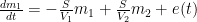
To start off, let’s review the argument I made, which is that the atmospheric-carbon-dioxide turnover time is what determined how long the post-bomb-test excess-carbon-14 level took to decay. That argument was based on the “bathtub” model, which Fig. 1 depicts. The rate at which the quantity <i>m</i> of water the tub contains changes is equal to the difference between the respective rates <i>e</i> (emissions) and <i>u</i> (uptake) at which water enters from a faucet and leaves through a drain:

The same thing can, <i>mutatis mutandis</i>, be said of contaminants (read carbon-14) in the water. But in the case of well-mixed contaminants one of the <i>mutanda</i> is that the rate at which the contaminants leave is dictated by the rate at which water leaves:

where 

Consequently, if the water quantity increases for an interval during which <i>e</i> exceeds <i>u</i>, it will thereafter remain elevated if the emissions rate <i>e</i> then falls no lower than the drain rate <i>u</i>. If a dose of contaminants is added to the water, though, the resultant contaminant amount falls, even when there’s no difference between <i>u</i> and <i>e</i>, in accordance with the <i>turnover</i> rate, i.e., with the ratio of <i>u</i> to <i>m</i>. So, to the extent that this model reflects reality’s relevant aspects, we can conclude that the rate at which the carbon-14 concentration decays tells us nothing about what happens when total-CO2 emissions return to a “normal” level.
But among the foregoing model’s deficiencies is that it says nothing about a possible dependence of overall drain rate <i>u</i> on the water quantity <i>m</i>, whereas we may expect biosphere uptake (and emissions) to respond to the atmosphere’s carbon-dioxide content. Nor does it deal with the possibility that after contamination has flowed out the drain it will be recycled through the faucet. In contrast, the biosphere no doubt returns to the atmosphere at least some of the carbon-14 it has previously taken from it.

A model that takes such factors into account could support a conclusion different from the one to which the bathtub led us. Consistently with my last post’s approach, Fig. 2 uses interconnected pressure vessels to represent one such model. In this case there are only two vessels, the left one representing the atmosphere and the right one representing carbon sinks such as the ocean and the biosphere.
The vessels contain respective quantities 


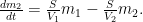
Those equations tell us that the carbon quantity 
![m_1(t) = \left[ \frac{V_1}{V_1+V_2}+\frac{V_2}{V_1+V_2} \exp\left(-\frac{V_1+V_2}{V_1V_2}St \right)\right] m_0 ,](https://s0.wp.com/latex.php?latex=m_1%28t%29+%3D+%5Cleft%5B+%5Cfrac%7BV_1%7D%7BV_1%2BV_2%7D%2B%5Cfrac%7BV_2%7D%7BV_1%2BV_2%7D+%5Cexp%5Cleft%28-%5Cfrac%7BV_1%2BV_2%7D%7BV_1V_2%7DSt+%5Cright%29%5Cright%5D+m_0+%2C+&bg=ffffff&fg=000&s=0&c=20201002)
which the substitutions 

Note that in the Fig. 2 system any constituent of the gas would be exchanged between vessels in accordance with the partial-pressure difference of that constituent alone, as if it were the only component the vessels contained. By thus constraining the flow from (and to) the first, atmosphere-representing vessel, this model supports the conclusion that the overall-carbon-dioxide quantity would, contrary to my previous argument, decay just as the excess, bomb-caused quantity of atmospheric carbon-14 did.

Could providing more than one sink enable us to escape that conclusion? Not necessarily. Consider the more-complex system that Fig. 3 depicts. Just as the system that my previous post described, this one can embody the TAR Bern-model parameters. As that post indicated, describing such a system requires a fourth-order linear differential equation. So that system does have more degrees of freedom in its initial conditions and can therefore exhibit a wider range of responses.
But it still constrains the flow among its four vessels linearly in accordance with partial pressures, just as the Fig. 2 system does. From complete equilibrium, therefore, its behavior for any constituent is the same as for any other constituent as well as for the contents as a whole. In other words, this model, too, seems to support the notion that the bomb-test results do indeed tell us how long excess carbon dioxide will remain if we stop taking advantage of fossil fuels.
In a sense, though, the models of Figs. 2 and 3 beg the question; they use the same uptake- and emissions-process-representing
So one question is how significant that difference is in the present context. I don’t have the answer, although my guess is, not very. But readers attempting to answer that question could do worse than start by referring to a previous WUWT post by Ferdinand Engelbeen.

Another way in which carbon-14 differs from the other two carbon isotopes is that it’s unstable. So, if the Fig. 3 model is adequate for carbon-12 or -13, a different model, which Fig. 4 depicts, would have to be used for carbon-14 if its radioactive decay is significant. That diagram differs from Fig. 3 in that it includes a flow 
To the extent that those different models produce different responses, using bomb-test data to predict the total carbon content’s behavior is problematic. But the Engelbeen post mentioned above seems to say that even deep-ocean residence times tend to be only a minor fraction of carbon-14’s half-life: this factor’s impact may be small.
A possibly more-significant factor is that the carbon cycle is undoubtedly non-linear, whereas the conclusions we tentatively drew from the models above depend greatly on their linearity. Before I reach that issue, though, I should point out an aspect of the Bern model that was not relevant to my previous post. The Bern equations I set forth in my last post were indeed linear. But that does not mean that their authors meant to say that the carbon cycle itself is. Although for the sake of simplicity I’ve discussed the models’ physical quantities as though they represented, e.g., the entire mass of carbon in a reservoir, their authors no doubt intended their (linear) models’ quantities to represent only the differences from some base, pre-industrial values. Presumably the purpose was to limit their range enough that the corresponding real-world behavior would approximate linearity.
But such linearization compromises the conclusions to which the models of Figs. 2 and 3 led us. A linear system is distinguished by the fact that its response to a composite stimulus always equals the sum of its individual responses to the stimulus’s various constituents; if the stimulus equals the sum of a step and a sine wave, for example, the system’s response to that stimulus will equal the sum of what its respective responses would have been to separate applications of the step and the sine wave. And this “superposition” property was central to drawing the conclusions we did from those models: the response to a large stimulus is proportionately the same as the response to a small one.

To appreciate this, consider Fig. 5, which depicts scaled values of the Fig. 2 model’s left-vessel total-carbon and carbon-14 contents. Initially, the system is at equilibrium, with zero outside emissions 


At time t = 5, a bolus of carbon-14 appears in the (atmosphere-representing) left vessel. Compared with the total carbon content, the added quantity is tiny, but it is large enough to double the small existing carbon-14 content. As the distance between the red dotted vertical lines shows, the resultant increase in carbon-14 content decays toward its new equilibrium value with a time constant of just about seven years. (I’ve assumed that the processes greatly favor the sink-representing right vessel—i.e., that its “volume” is much greater than the left vessel’s—so that the new equilibrium value is not much greater than the original.)
Now consider what happens at t = 45, when the left vessel’s total-carbon quantity suddenly increases. Although the two quantities are scaled to their respective initial values, this total-carbon increase is orders of magnitude greater than the t = 5 carbon-14 increase. Yet, as the black dotted vertical lines show, the decay of the left vessel’s total-carbon content proceeds just as fast proportionately as the much-smaller carbon-14 content did. As was observed above, this could tempt one to conclude that the carbon-14 decay we’ve observed in the real world tells us how fast the atmosphere would respond to our discontinuing fossil-fuel use.
![clip_image009[1]](http://wattsupwiththat.files.wordpress.com/2013/12/clip_image0091.png?quality=75 "clip_image009[1]")
But now consider what can happen if we relax the linearity assumption. Specifically, let’s say that the Fig. 2 model’s proportionality “constant”

In that plot, the red lines show that the carbon-14 decay occurs just as fast as in the previous plot, the carbon-14 content falling to exp(-1) above its new equilibrium value in around seven years. But the much-larger total-carbon increase brings the system into a lower-efficiency range, so that quantity subsides at a more-leisurely pace, taking over forty years. If such results are any indication, bomb-test results are a poor predictor of how long total-carbon content will settle.
Now permit me a digression in which I attempt to forestall pointless discussion of precisely what the quantities are that the graphs show. I believe the exposition is clearest if it is directed, as in Figs. 5 and 6, to ratios that carbon 14 and total carbon bear to their own initial values. But it appears customary to express the carbon-14 content instead in terms of its ratio to total carbon content. This means that, since total carbon has been increasing, the numbers commonly used in carbon-14 discussions could fall below the pre-bomb values, even though total carbon-14 has in fact increased.
For the sake of those to whom that issue looms large, I have attached Fig. 7 to illustrate how the values for carbon-14 itself could differ from those of its ratio to total carbon in a situation in which new (carbon-14-depleted) carbon is continually injected into the atmosphere.

But that’s a detail. More important is the issue that Fig. 6 raises.
Now, I “cooked” Fig. 6’s numbers to emphasize the point that nonlinearity can undermine conclusions based on linear models. Specifically, Fig. 6 depicts the results of making the flows proportional only to the fifth root of the carbon content.
But non-linearity must have some effect. How much? I don’t know. Together with the differences in behavior between carbon-14 and its stable siblings, though, it is among the considerations to take into account in assessing how informative the bomb-test data are.
As I warned at the top of the post, this post draws no conclusions from these considerations. But maybe the foregoing analysis will prompt knowledgeable readers’ comments that help narrow the issues.
DocMartyn says:
December 14, 2013 at 4:24 pm
“temperature controlled equilibrium”
Ok Fuck it. I am out of here
Doc, over 800,000 years there was a temperature controlled equilibrium of 8 ppmv/K, as can be seen in ice cores with resolution from less than a decade (Law Dome over the past 150 years) to 600 years (Vostok, 420 kyr) and 560 years (Dome C – 800 kyr):
http://www.ferdinand-engelbeen.be/klimaat/klim_img/Vostok_trends.gif
and for the MWP-LIA transition, see:
http://www.ferdinand-engelbeen.be/klimaat/klim_img/law_dome_1000yr.jpg
The increase after ~1850 is beyond the temperature controlled setpoint…
On a different note, may one ask why you think that your plot of emissions vs. atmospheric carbon is completely linear, yet you insist that CO2 absorption and emission from the oceans is dependent on SST and up/down welling? You cannot see a big change between 1995 and 2005.
CO2 absorption and uptake depends of the pCO2 difference and the mixing speed between atmosphere and waters.
Mixing speed is a function of wind speed.
pCO2 difference is a matter of pCO2 (~ppmv) in the atmosphere and temperature, total inorganic carbon (DIC), pH, salts content, etc. in seawater.
Temperature is the most important factor at the water side, followed by DIC. pH follows DIC, if no other external factors are involved.
The basic carbon exchange between atmosphere and deep oceans is via downwelling in cold polar area and upwelling in the warm tropics. That simply follows the ocean currents, as migration of CO2 in seawater is much too slow to be the primary internal and external transport of CO2.
Most of the exchange is because of the high pCO2 difference at the upwelling sites: up to 750 μatm vs. 400 μatm (~400 ppmv) in the atmosphere and at the downwelling sites: down to 150 μatm, again vs. 400 μatm in the atmosphere. That is what the basic 40 GtC/yr drives through the atmosphere and the deep oceans. Mostly a matter of winds which drives the circulation and density changes at the edge of the polar icefields.
A 10% change in the atmosphere, like from 400 to 440 ppmv will drive more CO2 in the downwelling sites, and at the same time reduce the release of CO2 (I know, you don’t believe that, but it is real physics, see Henry’s law) at the upwelling sites. The net result is an increase in uptake of a few % of the 10% change in the atmosphere, not a 10% increase…
David A says:
December 15, 2013 at 4:30 am
Assuming (Of course a large assumption) a 200 ppm spike above equilibrium, and then assuming humans have moved to non fossil fuel based power generation, then for how many years would this 0.1 GtC/yr growth in biomass continue until a new biomass equilibrium occurred.
Assuming a linear decay of the spike by all uptake mechanisms (oceans + vegetation) until the difference with the equilibrium is negligible (~6 half times), with a ~40 year half life time, that gives ~240 years of extra growth, most in the first years and decreasing over time.
If we may assume that the compartiment distribution of the peak 200 ppmv (424 GtC) extra remains the same as today for 110 ppmv above equilibrium (1 GtC/yr vegetation vs. 3.5 GtC/yr oceans), then over the 240 years some 100 GtC is extra absorbed by vegetation in growth and/or expansion and/or density. That is an increase of near 20% in land vegetation, if not limited by other factors…
gymnosperm says:
December 14, 2013 at 5:50 pm
I don’t think you can convert 12/13 ratios to GT except in the modern (Pleistocene) context because the carbon pie was much bigger in the past due to less deep ocean sequestration et al. Talking purely ratio, what would it take to get an 11 0/00 delta 13 excursion today?
Indeed, the sitations in current CO2 starved times and the geological past are not comparable. For the amounts necessary to reduce the atmospheric δ13C level with 8 per mil, that is not that simple, as the deep oceans give a lot of high δ13C CO2 back into the atmosphere (~40 GtC/yr):
http://www.ferdinand-engelbeen.be/klimaat/klim_img/deep_ocean_air_zero.jpg
The deep ocean exchanges did keep the atmosphere at ~-6.4 per mil in pre-industrial times with ~40 GtC/yr exchange rate. Human emissions are at -24 per mil average. To lower the per mil of the atmosphere with 11 per mil to -17.4 per mil, you have to emit some 40 GtC from fossil fuels per year.
Myrrh says:
December 14, 2013 at 5:14 pm
Myrrh, please read some basic textbooks about solubility of gases in liquids before making conclusions which don’t hold.
The maximum solubility of CO2 in fresh water at 1 bar CO2 (and nothing else) and 0°C is 3.3 g/l. The solubility of any gas is proportional to its own partial pressure in the atmosphere above the liquid surface, whatever the rest of the atmosphere. The partial pressure of CO2 in the atmosphere is 0.0004 bar. That makes that at 0°C some 1.32 mg/l CO2 is dissolved in rainwater, including the formation of carbonic acid, bicarbonate ions, carbonate ions and hydrogen ions. The latter make that raindrops are slightly acidic.
That is all, not even measurable in the atmosphere where the drop are formed.
It means that every 8-10 days water is washing carbon dioxide out of the atmosphere!
It is two-way traffic: what is emitted together with water vapour is returned back with water drops. Net effect: no change.
Heavier than air gases like carbon dioxide will always sink and lighter than air gases like water vapour and methane will always rise.
Much heavier particles like sand from the Gobi desert (hundreds of time heavier than air) are transported to Arizona, 6000 km farther. And you think that CO2, only 1.5 times heavier than air will sink out of the atmosphere?
Heavier than air gases like carbon dioxide will always sink and lighter than air gases like water vapour and methane will always rise.
What that is saying, to me, is that the amount in slow cycle of water weathering rocks is irrelevant to what comes next in the paragraph…
..which is saying that the fast cycle is more than adequately capable of mopping up whatever ‘man made’ can throw up there, and, that amount taken out of the atmosphere says nothing about limitation to the amount which can be taken out by the fast cycle.
The rock waethering cycle is a slow cycle, because the amounts of carbon cycling with the water cycle are small, 1-2 orders smaller than human emissions.
The fast cycle is the seasonal cycle, where lots of CO2 are moving in and out within a few month. But cycles do move CO2, they don’t necessary remove CO2. That is only the case if there is a difference between inputs and outputs. The net result of the fast cycle (in the ocean surface and vegetation) is limited, it is the medium fast cycle into the deep oceans which removes a lot, but still only about halve of the extra CO2 in the atmosphere induced by humans per year.
Ferdinand,
Well, four times our current production is within the realm of possibility but would be a very impressive effort. My point is that biological activity in the oceans appears to have produced shifts of this order in the past.
The entire range of 13C per mil values in carbonate rocks is about 20, ranging from +8 to -12. The mantle source is thought to be about -6. Our atmosphere (and if you are correct the mixed layer of the ocean) are about -8 today.
The Triassic excursion (the largest of three) when it was very hot went from -2 to +8 and back to -3 in phases of less than a million years.
The largest excursion was in the Neoproterozoic when it was cold and life was confined to the oceans. It went from +5 to -12 and back in about five million years.
You are probably right, and if our haphazard measurements of ocean exchange are anywhere near correct, you are almost certainly right. But the uncertainty of these measurements and the evidence of significant marine biological influence on isotope ratios in the past still lead me to suspect that better measurements of ocean/atmosphere exchange will hold big surprises for our conception of the Carbon cycle.
Ferdinand, IF Levine et al (and presumably the Berne model) are correct in concluding that the continuing decay in the 14C spike is being driven largely by dilution with continually added fossil-fuel 12C, then would you expect the decline to continue below the pre-bomb spike baseline?
Presumably this would happen in the next few years if nothing else changes significantly (other than continuing CO2 from anthropogenic sources which seems like a racing certainty to carry on at similar or increased levels).
Your patience is always appreciated.
Ferdinand Engelbeen says:
December 13, 2013 at 8:41 am
It doesn’t work like that. Using your mass decay estimate of 40% in 60 years in my equations, k would be .01527 (45y t1/2), I have worked out a fit of Mauna Loa and ORNL hCO2 since 1751 for a 42 year t1/2 (1/e in 60y) in which hCO2 accounts for all of the atmospheric CO2 increase. The fit using what I think are close to your parameters works, sort of, but there are problems.
I assumed a 280 ppmv in 1600, and ORNL total hCO2 emissions amounts to 1300 Gton through 2010. I am using an exponential fit (R^2 .988) of the ORNL estimates. A manual fit indicates the total hCO2 in the atmosphere now would have to be over 800 Gton. The results are clearly only good in the middle of the Mauna Loa data from 1959. The estimate of current total CO2 ppmv is higher than Mauna Loa. Another serious problem with the ~40 year t1/2 is the CO2 flux from reservoirs to the atmosphere would be only about 41 Gtons/yr. Few people would believe that figure. The extrapolation of exponentially increasing hCO2 is expected to quickly shoot well above the Mauna Loa extrapolation.
The ~40 year t1/2 view has implicit features that I suspect, like Hansen, will eventually be shown inaccurate due to implicit predictions. I give it another decade or two.
NUMBERS
Here are the ORNL emissions estimates and the hCO2 in atmosphere with 42y t1/2
t0 is 1600 [=Ho*EXP(k*(YR-1600)) + hCO2(y) * corr ], hCO2(y) is in the 3rd column.
k = -0.0167
corr = 0.9917 to handle Excel iteration error
h = 0.034819875 (I didn’t change this at all)
Ho =2.60337E-05 (I adjusted the curve down a little to fit recent emissions better)
1000 tons Gtons Gtons Gtons
Year C emissions hCO2/Y hCO2 in atm total hCO2 emitted since 1751
1959 2359659 8.652083 188.412317 297.2096123
1960 2485871 9.114860333 194.3311658 306.3244727
1961 2484985 9.111611667 200.1487689 315.4360843
1962 2573174 9.434971333 206.1907005 324.8710557
1963 2719685 9.972178333 212.665318 334.843234
1964 2857858 10.47881267 219.5351364 345.3220467
1965 2991515 10.96888833 226.7771896 356.290935
1966 3127493 11.46747433 234.3937524 367.7584093
1967 3223819 11.82066967 242.2344387 379.579079
1968 3399720 12.46564 250.5848899 392.044719
1969 3628311 13.303807 259.6282568 405.348526
1970 3931713 14.416281 269.6250939 419.764807
1971 4090118 14.99709933 280.0323677 434.7619063
1972 4278214 15.68678467 290.9512442 450.448691
1973 4503830 16.51404333 302.5096819 466.9627343
1974 4494028 16.47810267 313.8410543 483.440837
1975 4499752 16.49909067 325.0055779 499.9399277
1976 4747485 17.407445 336.8860171 517.3473727
1977 4887042 17.919154 349.0771623 535.2665267
1978 5072054 18.59753133 361.7391527 553.864058
1979 5209090 19.09999667 374.6897386 572.9640547
1980 5188499 19.02449633 387.350972 591.988551
1981 5054184 18.532008 399.3141178 610.520559
1982 5030048 18.44350933 410.9913739 628.9640683
1983 5085080 18.64529333 422.6753484 647.6093617
1984 5236615 19.20092167 434.7168373 666.8102833
1985 5426782 19.89820067 447.2503948 686.708484
1986 5502144 20.174528 459.8504137 706.883012
1987 5698733 20.89535433 472.9566031 727.7783663
1988 5917728 21.698336 486.6420534 749.4767023
1989 6008874 22.032538 500.4322827 771.5092403
1990 5911201 21.67440367 513.6389656 793.183644
1991 6087163 22.31959767 527.2667672 815.5032417
1992 5998683 21.995171 540.3471404 837.4984127
1993 6042268 22.15498267 553.3693705 859.6533953
1994 6069597 22.255189 566.2753098 881.9085843
1995 6181137 22.664169 579.373095 904.5727533
1996 6354251 23.29892033 592.8834465 927.8716737
1997 6376542 23.380654 606.2511038 951.2523277
1998 6305451 23.119987 619.1388715 974.3723147
1999 6371737 23.36303567 632.054232 997.7353503
2000 6560965 24.05687167 645.4437742 1021.792222
2001 6607764 24.228468 658.7817399 1046.02069
2002 6711648 24.609376 672.2765576 1070.630066
2003 7093542 26.009654 686.9365389 1096.63972
2004 7462233 27.361521 702.6943779 1124.001241
2005 7666095 28.109015 718.932536 1152.110256
2006 7920450 29.04165 735.8266627 1181.151906
2007 8151708 29.889596 753.2819084 1211.041502
2008 8287658 30.38807933 770.9424179 1241.429581
2009 8254587 30.266819 788.190192 1271.6964
2010 8630391 31.644767 806.5188311 1303.341167
The fit
C = N/K * (1 – e ^ -kt ) + Ho/(h+k) * (e ^ ht – e ^ -kt ) + (N + Ho) * e ^ -kt
N = 41 Gton/yr
k = -0.0167
h = 0.034819875
Ho = 2.60337E-05 Gton in 1600 (you have to let the system approach equilibrium)
Mauna Loa 42y t1/2
year ppmv fit ppmv
1959 315.97 316.7453998
1960 316.91 317.346574
1961 317.64 317.9684153
1962 318.45 318.6116665
1963 318.99 319.2770966
1964 319.62 319.9655015
1965 320.04 320.6777054
1966 321.38 321.4145614
1967 322.16 322.1769526
1968 323.04 322.9657932
1969 324.62 323.78203
1970 325.68 324.6266427
1971 326.32 325.5006459
1972 327.45 326.4050899
1973 329.68 327.341062
1974 330.18 328.3096879
1975 331.08 329.3121332
1976 332.05 330.3496045
1977 333.78 331.423351
1978 335.41 332.5346662
1979 336.78 333.6848891
1980 338.68 334.8754061
1981 340.1 336.1076526
1982 341.44 337.3831148
1983 343.03 338.7033314
1984 344.58 340.0698953
1985 346.04 341.484456
1986 347.39 342.9487213
1987 349.16 344.4644591
1988 351.56 346.0335002
1989 353.07 347.65774
1990 354.35 349.3391408
1991 355.57 351.0797346
1992 356.38 352.8816252
1993 357.07 354.7469907
1994 358.82 356.6780864
1995 360.8 358.6772475
1996 362.59 360.7468915
1997 363.71 362.8895219
1998 366.65 365.1077304
1999 368.33 367.4042009
2000 369.52 369.7817118
2001 371.13 372.2431402
2002 373.22 374.791465
2003 375.77 377.4297704
2004 377.49 380.16125
2005 379.8 382.9892103
2006 381.9 385.9170751
2007 383.76 388.9483892
2008 385.59 392.0868229
2009 387.37 395.3361768
2010 389.85 398.7003857
2011 391.63 402.183524
2012 393.82 405.7898103
michael hart says:
December 15, 2013 at 11:23 am
Ferdinand, IF Levine et al (and presumably the Berne model) are correct in concluding that the continuing decay in the 14C spike is being driven largely by dilution with continually added fossil-fuel 12C, then would you expect the decline to continue below the pre-bomb spike baseline?
Presumably this would happen in the next few years if nothing else changes significantly (other than continuing CO2 from anthropogenic sources which seems like a racing certainty to carry on at similar or increased levels).
Your patience is always appreciated.
Thanks Michael!
In the period up to the bomb spike, the dilution was from zero-14C human emissions, but most of the 14C bomb spike dilution is from the mixing in of pre-bomb spike deep ocean waters, minus the radioactive decay rate of about 10% over the time span of ~1000 years between downwelling and upwelling.
But as we ar near pre-bomb levels again, human emissions certainly will drop the 14C levels below the pre-bomb level, depending of how fast the emissions increase over time (or not).
On the other side, once the 14C levels drop below the return level of 14C from the deep ocean upwelling, this will dilute the human “fingerprint” of 14C, as good as is already the case for 13C…
Hoser says:
December 15, 2013 at 12:18 pm
To begin with, the 40 GtC is quite realistic, as that is the exchange rate between atmosphere and deep oceans only. There are larger seasonal exchange rates between the atmosphere and the ocean mixed layer (~50 GtC/yr) and vegetation (~60 GtC/yr), but these are quite readily in equilibrium with the atmosphere (1-2 years for ocean surface, somewhat longer for vegetation). That is the case for both 14C/12C ratio changes as for 13C/12C ratio changes.
Thus while the exchange rates are huge for vegetation and ocean surface, the redistribution of isotopic changes is finished after a few years, for the 14C bomb spike already before 1960, for the ocean surface, for vegetation somewhat later. Thus only the 40 GtC exchange with the deep oceans is what did give the decay rate of the 14C bomb spike and the thinning of the 13C/12C ratio (thus what rests of the human emissions in the atmosphere) to 1/3rd of the human contribution.
Further, the decay rate of the extra mass of CO2 and the decay rate of the isotopic composition are two totally different (and largely independent) things: the total refresh rate is 150 GtC in/out on a total of 800 GtC in the atmosphere. Or a residence time of ~5 years.
The decay rate of an excess amount of CO2 is independent of the refresh rate (input, throughput, output), but only depends of the difference between input and output. That is in direct ratio with the extra pressure of CO2 above equilibrium, not the extra human emissions.
That makes that the increase in mass caused by the human emissions is a simple linear decay function:
Cincrease = hC – (Cmlo – Ceq)*e^(-kt)
where k = 0.025
Cmlo = measured CO2 at Mauna Loa
Ceq = equilibrium CO2 level for the temperature over the time period.
But that the remaining fraction of original hCO2 decays with a much faster rate:
hCfraction = hC* (1 – e^(-kt))
where k = 0.05
I am sure that there are errors in the formulae, as my math is from 45 years ago and hardly used since then…
Anyway you may understand what I mean: any increase in the atmosphere as mass (whatever the source) has a halve life time of ~40 years, independent of the exchange rates, but a lot of the original human induced CO2 molecules are replaced with natural CO2 molecules by the 40 GtC/yr exchange rate with the deep oceans, as is also the case for the 14CO2 molecules.
As I like to see the math visualised, here the graph of 160 years of emissions:
http://www.ferdinand-engelbeen.be/klimaat/klim_img/fract_level_emiss.jpg
where FA is the accumulated fraction of hC in the atmosphere (e-fold time 5.3 years if I remember well, seems too fast now), FL in the mixed layer, tCA the calculated increase in the atmosphere (with an e-fold time of 51.5 years if I remember well) and tCAobs the observed increase. No problem to fit the increase in the atmosphere with the calculated increase of CO2…
Calculated for the yearly growth rate, that gives:
http://www.ferdinand-engelbeen.be/klimaat/klim_img/dco2_em4.jpg
where the calculated sink rate for each year is substracted from the emissions.
(BTW, the increase of emissions, the increase in the atmosphere and the sink rate are all three slightly quadratic, which makes that the derivatives all have relative linear slopes.)
Ferdinand Engelbeen says:
December 15, 2013 at 6:12 am
Myrrh says:
December 14, 2013 at 5:14 pm
Myrrh, please read some basic textbooks about solubility of gases in liquids before making conclusions which don’t hold.
The maximum solubility of CO2 in fresh water at 1 bar CO2 (and nothing else) and 0°C is 3.3 g/l. The solubility of any gas is proportional to its own partial pressure in the atmosphere above the liquid surface, whatever the rest of the atmosphere. The partial pressure of CO2 in the atmosphere is 0.0004 bar. That makes that at 0°C some 1.32 mg/l CO2 is dissolved in rainwater, including the formation of carbonic acid, bicarbonate ions, carbonate ions and hydrogen ions. The latter make that raindrops are slightly acidic.
That is all, not even measurable in the atmosphere where the drop are formed.
Not even measurable? There is enough to turn all rainwater acid.., and that’s only from the around 1% of the carbon dioxide in solution which goes on to form carbonic acid.
Perhaps it is better expressed as 90 cm3 of CO2 per 100 ml water…?
Water and carbon dioxide are greatly attracted to each other..
“It means that every 8-10 days water is washing carbon dioxide out of the atmosphere!”
It is two-way traffic: what is emitted together with water vapour is returned back with water drops. Net effect: no change.
That is patent nonsense. A volcanic eruption propelling tons of carbon dioxide into the atmosphere is not going to return to the atmosphere in like mass once it has come back to the surface in solution through precipitation or gravity!
What? is your strange ocean and land repelling it somehow? By what mechanism?
“Heavier than air gases like carbon dioxide will always sink and lighter than air gases like water vapour and methane will always rise.”
Much heavier particles like sand from the Gobi desert (hundreds of time heavier than air) are transported to Arizona, 6000 km farther. And you think that CO2, only 1.5 times heavier than air will sink out of the atmosphere?
Of course it sinks out of the atmosphere! That’s what gravity does to anything with mass that is heavier than air – that’s why you find the sand deposited on your car..
“Heavier than air gases like carbon dioxide will always sink and lighter than air gases like water vapour and methane will always rise.
“What that is saying, to me, is that the amount in slow cycle of water weathering rocks is irrelevant to what comes next in the paragraph…
“..which is saying that the fast cycle is more than adequately capable of mopping up whatever ‘man made’ can throw up there, and, that amount taken out of the atmosphere says nothing about limitation to the amount which can be taken out by the fast cycle.”
The rock waethering cycle is a slow cycle, because the amounts of carbon cycling with the water cycle are small, 1-2 orders smaller than human emissions.
The fast cycle is the seasonal cycle, where lots of CO2 are moving in and out within a few month. But cycles do move CO2, they don’t necessary remove CO2. That is only the case if there is a difference between inputs and outputs. The net result of the fast cycle (in the ocean surface and vegetation) is limited, it is the medium fast cycle into the deep oceans which removes a lot, but still only about halve of the extra CO2 in the atmosphere induced by humans per year.
Rain and weight of carbon dioxide are the two main methods carbon dioxide is removed from the atmosphere in all cycles, and so in the short cycle – if it were not so you wouldn’t have any seasonal cycles, you would have what you erroneously claim – a build up, an accumulation of carbon dioxide in the atmosphere – and that is clearly what we do not have.
We do not have millenniums worth of carbon dioxide saturating the atmosphere because you have no way of getting it to the “sinks”..
Although I’ve been able to take some time this morning to assemble the data to which DocMartyn directed me, it’s likely that this thread’s activity will wind down before I will get around to replicating his work or modeling what Mr. Engelbeen has explained.
But I don’t want to let the opportunity pass to thank Mr. Engelbeen, DocMartyn, and others on this thread again for an enlightening exchange and in particular to Mr. Engelbeen for his patience. To me the discussion has really been helpful (even though I agree with the sentiment others have expressed that, as far as the ultimate issue is concerned, it doesn’t matter much how long enhanced CO2 concentrations persist).
I need to chew on the numbers, but I have to do other things.. I may try to contact you directly since I’m not sure when I’ll get back to you. This has been a very good back-and-forth.
Pre addendum
Ferdinand Engelbeen says:
December 15, 2013 at 4:20 pm
Hoser says:
December 16, 2013 at 6:24 am
I need to chew on the numbers, but I have to do other things.. I may try to contact you directly since I’m not sure when I’ll get back to you.
Please contact me, so that I can send you the Excel file with the calculations for the graphs, if I can find it back (it’s already from a few years ago…)…
Joe Born says:
December 16, 2013 at 4:44 am
You are welcome. It is always a pleasure to meet people who want to know and with whom we can have a nice discussion. Then the knowledge is increasing at both ends of the Internet…
Monckton of Brenchley wrote: “Why is half of all the CO2 we emit disappearing instantaneously from the atmosphere?”
Half of the CO2 we emit is not disappearing INSTANTANEOUSLY, on average about half the CO2 we emit is taken up by the oceans and terrestrial biota, but if you look at the proportion of our CO2 that is taken up each year (which we know via conservation of mass) it varies greatly from year to year. The natural environment has no way of “knowing” how much CO2 we emit each year; the key physics depends on the total amount of CO2 in the atmosphere, and it is that to which the natural sources and sinks are responding.
“I’d be most grateful if wiser heads than mine were able to explain that.”
As to why it happens, the scientific evidence suggests it is mostly ending up in the oceans. The solubility of CO2 in the oceans is proportional to the difference in partial pressure between the surface waters and the atmosphere. If we increase atmospheric CO2 via fossil fuel emissions, this difference will rise and the oceans will increase the uptake of CO2. This is supported by the observation that the oceans are acidifying (or becoming less alkaline for the pedantic). As to why the proportion is approximately constant, if you model the carbon cycle with a first order differential equation, you find that approximately exponentially increasing fossil fuel emissions result in an approximately exponential increase in excess atmospheric CO2, and the ratio of the two is a constant. While the carbon cycle is non-linear, and our emissions are not rising exactly exponential, the model is sufficiently close to give a reasonable qualitative explanation of what is going on. There is an example of such a model in the paper that I wrote specifically to address the “residence time argument” that seems to take up such an inordinate amount of space on climate blogs, given the actual level of scientific uncertainty. You can get the paper here:
Gavin C. Cawley, “On the Atmospheric Residence Time of Anthropogenically Sourced Carbon Dioxide”, Energy Fuels, 2011, 25 (11), pp 5503–5513 (http://pubs.acs.org/doi/abs/10.1021/ef200914u)
I just want to say that I am always amazed and impressed by Ferdinand’s energy and enthusiasm in explaining the science of the carbon cycle and also the moderate and pleasant tone he adopts, keep up the good work Ferdinand!
@Myrrh
Ferdinand said this in an earlier discussion and repeats it here:
“The maximum solubility of CO2 in fresh water at 1 bar CO2 (and nothing else) and 0°C is 3.3 g/l. The solubility of any gas is proportional to its own partial pressure in the atmosphere above the liquid surface, whatever the rest of the atmosphere. The partial pressure of CO2 in the atmosphere is 0.0004 bar. That makes that at 0°C some 1.32 mg/l CO2 is dissolved in rainwater, including the formation of carbonic acid, bicarbonate ions, carbonate ions and hydrogen ions. The latter make that raindrops are slightly acidic.
That is all, not even measurable in the atmosphere where the drop are formed.”
Here is more on the subject:
“Rainwater in particular, with its high surface area, picks up a lot of CO2 as it falls.” from http://www.marietta.edu/~mcshaffd/aquatic/sextant/chemistry.htm
Ferdinand’s 1.32 mg/litre is 1.32 ppm(m) or 1.32 g/cubic metre water. I was unable to come up with a number that low even ignoring the carbonic acid and carbonate ions.
Between 30 Deg N and S with an average rainfall of about 1.5 metres p.a. the volume is about:
37,500 km avg circumference, (3340 x 2) km north to south x 1000m x 1000m x 1.5m of rain = 3.75 x 10^14 cubic metres of rain. With 1.32 g/cubic metre the total is only 500 millions tons of CO2 p.a. in that zone. That doesn’t seem like much.
http://www.seafriends.org.nz/oceano/seawater.htm reports that the CO2 content of sea water is 90 mg/kg, or 92 g per cubic metre – a very much higher number. Fresh water holds about 20% more CO2 that sea water. So instead of 500 million it would be 35 billion tons p.a.
But even that doesn’t add up with other figures on that same site. It says sea water contains 40 ml CO2/litre. 40 x 1.2 (for fresh water) = 48 ml/litre.
Willis reports that the concentration is over 400 ppm(v) in his discussion of CO2 in air and sea water http://wattsupwiththat.com/2013/11/27/co2-in-the-air-co2-in-the-seawater It is clear that Ferdinand’s value for CO2 in water droplets is probably low. I have also seen referenced 600 ppm(m) for seawater and >1100 for fresh water.
So what is the equilibrium CO2 concentration, on a mass basis, of rainwater?
Crispin in Waterloo says:
December 16, 2013 at 10:09 am
Ferdinand’s 1.32 mg/litre is 1.32 ppm(m) or 1.32 g/cubic metre water. I was unable to come up with a number that low even ignoring the carbonic acid and carbonate ions.
That number is the absolute maximum solubility of CO2 in fresh water cold, near freezing at 0.0004 bar partial pressure of CO2 in the atmosphere and includes the chemical reactions of CO2 with water to form carbonic acid and further dissociation to carbonates and bicarbonates. See:
http://www.engineeringtoolbox.com/gases-solubility-water-d_1148.html
http://www.seafriends.org.nz/oceano/seawater.htm reports that the CO2 content of sea water is 90 mg/kg, or 92 g per cubic metre – a very much higher number. Fresh water holds about 20% more CO2 that sea water.
I don’t know where the 20% more CO2 in fresh water than in seawater is coming from? Seawater holds many more times CO2 than fresh water, because it is alkaline and forms a buffer solution. The higher the pH, the more CO2 can be dissolved in water. You can dissolve a lot of sodium bicarbonate in fresh water, where the CO2 content is many times the maximum solubility of CO2 in fresh water, without any CO2 bubbling out of the solution. Add some acid until pH 5.6 (the pH of CO2 at 1 bar saturation in fresh water) and see what happens: near all CO2 comes out of the solution…
So what is the equilibrium CO2 concentration, on a mass basis, of rainwater?
1.32 mg/kg at 0.0004 bar pressure and 0°C. Less at lower air (and thus CO2) pressure, less at higher temperatures. Less if stronger acids (derived from NOx, SO2, SO3) are present.
agfosterjr says:
December 13, 2013 at 8:11 pm
Good Point ! Where’s an interactive analog computer simulator when you need one ? There’s a lot of remarkably clean information in the Mauna Loa data , http://upload.wikimedia.org/wikipedia/commons/8/88/Mauna_Loa_Carbon_Dioxide.png , and it would be great to be able to play with the minimal circuits capable of generating it . Maybe that’s what Joe presented in his box models , but my focus is on implementing the spherical spectral maps necessary to accurately compute the radiative balance with the sun which determines our mean temperature , and I don’t have the brain-spacetime left over to grok the coupled diff eqs . .
Considering that the jaggies reflect the difference between the seasonal , clearly biological , absorptions of the terrestrial and oceanic hemispheres , I’m impressed that this is enough to make the curve steeply decline . My intuition remains that the fact that the curve follows changes both down and up makes me unsurprised by a half life of 5 to 10 years .
Anyway , it’s been a discussion which evidences that this realist blogsphere is where serious web-speed peer review is happening ..
Crispin in Waterloo says:
December 16, 2013 at 10:09 am
Ferdinand’s 1.32 mg/litre is 1.32 ppm(m) or 1.32 g/cubic metre water. I was unable to come up with a number that low even ignoring the carbonic acid and carbonate ions.
..
So what is the equilibrium CO2 concentration, on a mass basis, of rainwater?
Maybe he’s just pulled that 1ppm out of the air.., perhaps on weight, water is 1gram/1ml.
Also, working in grams appears to be giving him an unrealistic concept of the amount of carbon dioxide, water is considerably heavier than gas.*
The standard figure I have given, at room temperature, transposes the gram/litre to a more easily recognisable amount:
“Perhaps it is better expressed as 90 cm3 of CO2 per 100 ml water…?”
900 cm3 per litre – that is not an isignificant volume of carbon dioxide. Colder temps will hold more but “room temp” might be thought of as a general average.
Anyone can pick up or imagine a standard ruler where 12″ is around 30 centimetres, three of those in height, width and breadth give the amount cubed of carbon dioxide in the scant 100 ml of water, multiply by ten to get 1 litre – that is a considerable area of carbon dioxide. 1 litre = 1.75 pints.
How does such a vast amount of carbon dioxide fit into 100ml of water? Because, contrary to the erroneous gospel of AGW, real physics teaches that gases are condensible, (their individual volumes expand when heated and condense when cooled, which is how we get our winds). All that carbon dioxide now in solution may only appear to be a minute amount in terms of weight but it came from a rather large volume in terms of carbon dioxide molecules.
Water the universal solvent with its great attractive powers pulls in any and all carbon dioxide around it for all practical purposes, and in precipitation brings that back to the surface in its 8-10 day cycle.
I don’t understand how it can be ignored that the Water cycle is constantly clearing the atmosphere of carbon dioxide, and what water doesn’t capture then gravity does.
There are lots of simple experiments detailed on line to show how carbon dioxide is heavier than air, creating it with a kitchen mix of bicarb of soda and vinegar and pouring it onto a lit candle in a jar will look amazing for adults as well as children as the candle is put out by this invisible force.. Use dry ice to see it in action because the invisible carbon dioxide mixes with water in the air and water vapour is visible, you will ‘see’ the carbon dioxide spilling over the sides of the glass as it makes the water vapour heavier. Dry ice is used to great atmospheric effect in the theatre as it changes from solid straight to gas at room temp for those misty foggy scenes.
*There is a bit of history involved in how ratios should be measured: http://dl.clackamas.cc.or.us/ch104-03/molecule.htm
AGW has destroyed all properties and processes of gases, reducing them to a ‘model’ without attraction and volume or weight so not subject to gravity, hence their peculiar ‘kinetic’ theory to get their ‘thoroughly mixed’. . That is why they can simply not include the Water Cycle and relative weight under gravity in the Carbon cycle, and the majority do not notice these are missing. Not even at university level.
They cannot explain winds with their model gases. We have a generation of ‘climate’ scientists without any knowledge of basic meteorology.
Myrrh says:
December 16, 2013 at 3:07 pm
Maybe he’s just pulled that 1ppm out of the air.., perhaps on weight, water is 1gram/1ml.
Myrrh, the maximum solubility of 1 bar CO2 in fresh water at °C is 3.3 g/kg:
http://www.engineeringtoolbox.com/gases-solubility-water-d_1148.html
that includes the subsequent reactions which transformes CO2 in carbonic acid, bicarbonates and carbonates.
But CO2 is not at 1 bar in the atmosphere. If the air is at 1 bar (at sealevel), then the partial pressure of CO2 is 0.0004 bar (400 ppmv CO2 / 1 million ppmv air). The solubility of any gas is directly in proportion to the partial pressure of that gas in the atmosphere, regardless of what the rest of the atmosphere is (full vacuum to 78% nitrogen and 21% oxygen and some 1% argon – 1 bar together):
http://en.wikipedia.org/wiki/Henry%27s_law
about partial pressure:
http://en.wikipedia.org/wiki/Partial_pressure
“Perhaps it is better expressed as 90 cm3 of CO2 per 100 ml water…?”
It looks more impressive if you express it in volumes of gas against liquid, but it is not:
Raindrops are formed from water vapour which is at some 2% in cold air at the height of clouds. To form 1 l (or kg) of rainwater, you need 400 m3 (1 m3 = 1000 liter) of air (if all present water condenses, which is never the case). The 900 cm3 of CO2 absorbed by 1 l of rainwater from 400 m3 of air is simply negligible in the total volume of CO2 present in 400 m3 of air: 400 m3 * 0.0004 = 0.16 m3 = 160 liter CO2 = 160,000 cm3 CO2 (1 l = 1 dm3 = 1000 cm3)…
Crispin in Waterloo says:
December 16, 2013 at 10:09 am
So what is the equilibrium CO2 concentration, on a mass basis, of rainwater?
At 25ºC fresh water in equilibrium with an atmosphere containing 350ppm CO2 it’s 0.52 mg/L, which gives a pH of ~5.6.
Myrrh says:
December 16, 2013 at 3:07 pm
Crispin in Waterloo says:
December 16, 2013 at 10:09 am
Ferdinand’s 1.32 mg/litre is 1.32 ppm(m) or 1.32 g/cubic metre water. I was unable to come up with a number that low even ignoring the carbonic acid and carbonate ions.
..
So what is the equilibrium CO2 concentration, on a mass basis, of rainwater?
Maybe he’s just pulled that 1ppm out of the air.., perhaps on weight, water is 1gram/1ml.
Also, working in grams appears to be giving him an unrealistic concept of the amount of carbon dioxide, water is considerably heavier than gas.*
The standard figure I have given, at room temperature, transposes the gram/litre to a more easily recognisable amount:
“Perhaps it is better expressed as 90 cm3 of CO2 per 100 ml water…?”
900 cm3 per litre – that is not an isignificant volume of carbon dioxide. Colder temps will hold more but “room temp” might be thought of as a general average.
No way, that’s high by orders of magnitude! The equilibrium value at 25ºC is about 12micromole/L or about 0.27cm^3/L.
AGW has destroyed all properties and processes of gases, reducing them to a ‘model’ without attraction and volume or weight so not subject to gravity, hence their peculiar ‘kinetic’ theory to get their ‘thoroughly mixed’. . That is why they can simply not include the Water Cycle and relative weight under gravity in the Carbon cycle, and the majority do not notice these are missing. Not even at university level.
Nothing to do with AGW, it’s standard kinetic theory of gases which has been a staple of physical chemistry and engineering for over a century, (Boyle and Charles’ Laws, Fick’s Law of Diffusion etc.) Myrrh has been repeatedly advised to read a phys chem textbook, most recently by Ferdinand but to no avail, he still keeps trotting out the same nonsense.
@ur momisuglyPhil
Thanks for the summation. I have of course used the Engineering Toolbox on hundreds of occasions and it is interesting to me to find outer sources that give different values. For example I have seen the CO2 content of sea water reported as 400 ppm and also 600 ppm which might be the volumetric v.s. mass bases comparison, assuming that the mass basis is treated as solid CO2 (which is about 1.56 to convert). The thing is references are not very complete and people happily mix metrics in a single paragraph.
I also came up with the same figure of 0.52 mg/Lit but for 400 ppm it is of course more.
0.52 mg/L is 520 ppm(m) which is not small.
@ur momisugly Ferdinand
“It looks more impressive if you express it in volumes of gas against liquid, but it is not:
Raindrops are formed from water vapour which is at some 2% in cold air at the height of clouds. To form 1 l (or kg) of rainwater, you need 400 m3 (1 m3 = 1000 liter) of air (if all present water condenses, which is never the case). The 900 cm3 of CO2 absorbed by 1 l of rainwater from 400 m3 of air is simply negligible in the total volume of CO2 present in 400 m3 of air: 400 m3 * 0.0004 = 0.16 m3 = 160 liter CO2 = 160,000 cm3 CO2 (1 l = 1 dm3 = 1000 cm3)…”
Well it looks LESS impressive if you choose a height at which there is not much water vapour. The condensation of humid air at sea level drops CO2 into the ocean much more effectively so the calculation above would look very different. I sense you are trying to minimize the actual amount of CO2 that is transferred into the oceans by water droplets. Why? The amount is huge and it is a significant (detectable) part of the carbon cycle. I can’t see any advantage in underrepresenting it.
The volume of air between sea level and 1000 m at the equator, 1000 km north and south is 77m cu km. Even at 2% that is 3×10^16 litres of CO2 trapped in the droplets. Air that is not visibly ‘cloudy’ has a great deal of 2 micron water droplets in it. I know because I have to avoid measuring them in the lab.
At sea level and 20 degrees the moisture level is 17g/m3 each evening and it condenses. At 35 degrees (hardly unknown in the tropics) it is 34.4 g/m3. Each evening it cools and a great portion of it drops into the sea. The near surface layer is highly active in evaporating and returning water to the sea. When it is in the air it picks up CO2 very rapidly. We are often told the gas interchange with the ocean is dominated by the surface area available (ocean surface). This is not true. Rain drops have a very large surface to volume ratio and are efficient scavengers.
Dr Bill Mollison once pointed out to me the large amount of condensation (dew) that in some places exceeds the ‘rainfall’ by a factor of 5. At the moment I am convinced that CO2 stripping by fresh water is responsible for the elevated warm water CO2 levels Willis found in his investigation into sea temps and CO2 a few weeks ago.
Crispin in Waterloo says:
December 17, 2013 at 12:34 pm
At sea level and 20 degrees the moisture level is 17g/m3 each evening and it condenses. At 35 degrees (hardly unknown in the tropics) it is 34.4 g/m3.
That probably is right (I haven’t looked it up), but sealevel in the tropics is also where a lot of CO2 is emitted continuously from the same warm waters where the water vapour comes out. What rain is doing is some of the extra CO2 releases bringing back to the surface. Most of it is simply recycling and one the main CO2 flows still is from the equator to the poles via the atmosphere and back via the deep oceans: ~40 GtC/yr. Other fluxes are mainly seasonal between ocean surface and atmosphere (~50 GtC back and forth) and between vegetation and atmosphere (~60 GtC back and forth) . Human emissions are ~10 GtC/yr and the carbon circulating through the water vapour cycle is ~0.5 GtC/yr.
The fast water cycle is lifting CO2 together with water vapour from the warm equatorial ocean surface and bring (some) back to the surface via rain. That is largely a negative operation: far less returns with rain in the tropics than what is emitted and ultimately reaches the polar sinks (and vegetation). What drops out over land is a much slower cycle and if the reference provided by Myrrh is right, only 0.01 to 0.1 GtC/yr is following that cycle.
Ferdinand Engelbeen says:
December 17, 2013 at 2:55 pm
The fast water cycle is lifting CO2 together with water vapour from the warm equatorial ocean surface and bring (some) back to the surface via rain. That is largely a negative operation: far less returns with rain in the tropics than what is emitted and ultimately reaches the polar sinks (and vegetation). What drops out over land is a much slower cycle and if the reference provided by Myrrh is right, only 0.01 to 0.1 GtC/yr is following that cycle
Lots of vegetation over the poles..
Do you think it is right? That reference said the way back into the atmosphere for carbon dioxide in the slow cycle is from volcanoes.
Timothy Casey has taken a look at the deceit rampant in producing figures from volcanic activity – http://carbon-budget.geologist-1011.net/
“Based on this brief literature survey, we may conclude that volcanic CO2 emissions are much higher than previously estimated, and as volcanic CO2 contributions are effectively indistinguishable from industrial CO2 contributions, we cannot glibly assume that the increase of atmospheric CO2 is exclusively anthropogenic.”
November 2013 http://www.worldcrunch.com/rss/default/japan-039-s-brand-new-island/volcano-earthquake-japan-island/m1c0s14164/
October 2013 http://www.worldcrunch.com/rss/default/russian-volcano-039-s-sky-high-eruption/volcano-ash-russia/m1c0s13782/
“Klyuchevskoy, the highest volcano in Asia, located in eastern Russia, spewed ash Friday up to an incredible estimated height of 10 kilometers, or 6.2 miles, Voice of Russia reports.
Local villagers saw ashes rain down on their houses, as the cloud travelled 124 miles southwest of the volcano. Klyuchevskoy, a 15,584 feet-high volcano which is just one among 150 other volcanos on the Kamchatka peninsula, has had regular eruptions over the last decade.”
Etc., etc. My emphasis italics..
The extent of the volcanic activity annually is unknown, in large part again as with temperature records, the numbers are hidden, manipulated. The actual figures of known eruptions are not used and particularly not used are the thousands of active underwater volcanoes, many more thousands have been found and are still being found. As Casey details, the estimates they do use are corrupt, deliberately so.
You still have the problem of showing how carbon dioxide is removed from the atmosphere since you don’t admit to gravity existing nor to the water cycle playing any significant part, so the build up just from those volcanoes which have erupted in the last hundred years must have pushed carbon dioxide levels in the atmosphere into the multiple thousands ppm….
..how much over millenniums?