Guest essay by Joe Born
Is the Bern Model non-physical? Maybe, but not because it requires the atmosphere to partition its carbon content non-physically.
![bern_irf[1]](http://wattsupwiththat.files.wordpress.com/2013/12/bern_irf1.gif)
A Bern Model for the response of atmospheric carbon dioxide concentration 


![\rho_{CO_2}(t)=C_{CO2}\int\limits_{-\infty}^{t}E_{CO_2}(t')\left[ f_{CO_2,0}+\sum\limits_{S=1}^{n} f_{CO_2,S}e^{-\frac{t-t'}{\tau_{CO_2,S}}} \right]dt' .](https://s0.wp.com/latex.php?latex=%5Crho_%7BCO_2%7D%28t%29%3DC_%7BCO2%7D%5Cint%5Climits_%7B-%5Cinfty%7D%5E%7Bt%7DE_%7BCO_2%7D%28t%27%29%5Cleft%5B+f_%7BCO_2%2C0%7D%2B%5Csum%5Climits_%7BS%3D1%7D%5E%7Bn%7D+f_%7BCO_2%2CS%7De%5E%7B-%5Cfrac%7Bt-t%27%7D%7B%5Ctau_%7BCO_2%2CS%7D%7D%7D+%5Cright%5Ddt%27+.&bg=ffffff&fg=000&s=0&c=20201002)
The “Bern TAR” parameters thus adopted state that the carbon-dioxide-concentration increment 

where the 


There are a lot of valid reasons not to like what that equation says, the principal one, in my view, being that the emissions and concentration record we have is too short to enable us to infer such a long time constant. What may be less valid is what I’ll call the “partitioning” version of the argument that the Bern model is non-physical.
That version of the argument was the subject of “The Bern Model Puzzle.” According to that post, the Bern Model “says that the CO2 in the air is somehow partitioned, and that the different partitions are sequestered at different rates. . . . Why don’t the fast-acting sinks just soak up the excess CO2, leaving nothing for the long-term, slow-acting sinks? I mean, if some 13% of the CO2 excess is supposed to hang around in the atmosphere for 371.3 years . . . how do the fast-acting sinks know to not just absorb it before the slow sinks get to it?” (The 371.3 years came from another parameter set suggested for the Bern Model.)
The comments that followed that post included several by Robert Brown in which he advanced other grounds for considering the Bern Model non-physical. As to the partitioning argument, though, one of his comments actually came tantalizingly close to refuting it. Now, it’s not clear that doing so was his intention. And, in any event, he did not really lay out how the circuit he drew (almost) answered the partitioning argument.
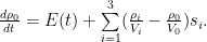
So this post will flesh the answer out by observing that the response defined by the “Bern TAR” parameters is simply the solution to the following equation:

where

But that equation describes the system that the accompanying diagram depicts. And that system does not impose partitioning of the type that the above-cited post describes.

In the depicted system, four vessels of respective fixed volumes 


Additionally, a gas source can add gas to the first vessel at a rate 

If appropriate selections are made for the 
The gas represents carbon (typically as a constituent of carbon dioxide, cellulose, etc.), the first vessel represents the atmosphere, the other vessels represent other parts of the carbon cycle, the membranes represent processes such as photosynthesis, absorption, and respiration, and the stimulus 
I digress here to draw attention to the fact that I’ve just moved the pea. The flow from the source does not represent all emissions, or even all anthropogenic emissions. It represents the flow only of carbon that had previously been sequestered for geological periods as, e.g., coal, and that is now being returned to the cycle of life. Thus re-defining the model’s emissions quantity finesses the objection some have made that the Bern Model requires either that processes (implausibly) distinguish between anthropogenic and natural carbon-dioxide molecules or that atmospheric carbon dioxide increase without limit.
Now, there’s a lot to criticize about the Bern Model; many of the criticisms can be found in the reader comments that followed the partitioning-argument post. Notable among those were richardscourtney’s . Also persuasive to me was Dr. Brown’s observation that the atmosphere holds too small a portion of the total carbon-cycle content for the 0.152 value assigned to the infinite-time-constant component to be correct. And much in Ferdinand Engelbeen’s oeuvre is no doubt relevant to the issue.
As the diagram shows, though, the left, atmosphere-representing vessel receives all the emissions, and it permits all of the other vessels to compete freely for its contents according to their respective membranes’ permeabilities. So what is not wrong with the model is that it requires the atmosphere to partition its contents, i.e., to withhold some of its contents from the faster processes so that the slower ones get the share that the model dictates.
Related articles
- On CO2 residence times: The chicken or the egg? (wattsupwiththat.com)
Plot the Soto Aerosol induced optical depth vs. [CO2] and see what happens when you add nutrients and flocculants to the Pacific Ocean; the June 1991 Mount Pinatubo eruption did.
ZP: ” I don’t believe that you are accurately representing their model or mathematics. For example, the authors have demonstrated an appreciation for the forward and reverse exchange rate constants being unique. Also, they did not derive a fourth-order differential equation from a system of first-order ODEs as you apparently have done.”
They gave a response, namely, the first equation above. The Bern TAR coefficients give a specific version of that response. That version is a solution to a scalar differential equation. Now, it was back during the Johnson administration that I fulfilled my college-math requirement, and I spent my career practicing law, not mathematics, so recent mathematical developments likely escaped my attention. If so, and the third equation above is no longer the one the TAR Bern equation solves, I will be grateful if you can tell me which one it solves now.
As to the implied invitation to show how I derived the third equation above, I decline. Setting it out would be tedious. And–you’re forcing me to be blunt here–your failure to recognize that the TAR Bern equation solves a fourth-order equation suggests to me that no further enlightenment on your part would justify the effort.
Maybe we should just agree to disagree.
Ferdi “Additional for 14C is that a huge part is directly absorbed but comes back in the next season with the fallen leaves, but that part is getting in more permanent storage + that the Nordkapp is practically in the middle of the largest sink place of the oceans.”
I picked the name Nordkap from a spreadsheet someone posted on another thread. It may be a complete misnomer apart from the the Norwegian connection. The Nydal dataset (see source URL on graphs) is from a number of sites across Europe and Africa including Madagascar.
http://cdiac.esd.ornl.gov/epubs/ndp/ndp057/ndp057.htm
I again draw your attention to the clear seasonal signal at the beginning of the record that dies off very quickly. This confirms your claim of a dilution effect but also clearly confines its impact to less than ten years.
Whether this is due to dead leaves or ocean surface, it’s clear that it is transitory with a time constant of the order of one for two years. (I hope to firm this up by cross-referencing different methods). Failing to account for the fast exponential and fitting just a single decay (as Gosta Pettersson was doing) seems to shorten the circa 17 year constant by a couple of years.
This all seems consistent with one set of Bern constants that I have seen 1.86 and 18.6 years but I see no evidence in this data of a longer period like the third Bern figure or your 51 year suggestion.
Since the Bern results are empirical rather than truly theoretically modelled, it seems that (at least one version of the story) it’s hitting figures that are supported by decay of atmospheric C14 levels.
It seems that the four box model is almost an arbitrary model of the right kind. It is likely that most of this can be characterised by linear relaxation models of something or other and by providing a range of box volumes (whether tentatively based of rough guesses of various ecosystem is somewhat immaterial) and providing a range of tunable parameters, it should be able to match something even if it is badly wrong in principal.
The fact that this can also approximate a diffusion relationship gives it even more scope.
Does anyone have any evidence of such a long decay period directly in any data?
Allan MacRae says:
“Thank you for your clarification Greg. I found your previous comments imprecise and impolite. ”
My initial comments on the thread where your paper was presented were unnecessarily dismissive. I corrected that later in the thread but you did not seem to follow the the discussion.
I apologise for appearing impolite, but I now have a very short fuse with having to deal with the defects of these bloody ubiquitous running-means everywhere and of that your study is guilty. You are using a filter that will _insert_ a spurious 9month signal into the data in a paper whose main point is the presence of a 9 month lagged correlation.
Fortuitously, this is not the cause of the effect and what you found turned out to be real when I repeated it with a half decent filter. Science is about validation and I reproduced and validated your result. I regard that as a positive contribution and suggest you view it in the same light and adopt one of the filters from my C.Etc article of another if you find one you prefer elsewhere.
Thank you for bringing attention to this correlation. It is not enough to prove that SST driving CO2 is the full story but it is an important element. I hope to have more on that very shortly.
best regards. Greg.
Because about half of human addition to the atmosphere is apparently “lost”, everyone wants to think of the biological cycle as only a sink, sucking 12CO2 from the atmosphere over land to produce lignin, and over the ocean to produce carbonate. What is missing is biological “production” of 12C. Marine creatures will mine HCOC3 for their carbonate (Klaus Keller, Francois Morel, 1999). Bacteria eat rocks…
? Extreme ultra high temperature (UHT) metamorphism? Sorry, not quite. Limestone is metamorphosed to marble as it re-crystallizes, dolomite may form marble, but under greater metamorphic conditions forms talc deposits. Dolomite has a greater magnesium content. Marble metamorphoses into calc-silicates. Mountain building and tectonic activity are the big drivers and I would place them as greater influences than contact metamorphosis which requires long contact with a magmatic body.
Further metamorphism is where the carbonate structures decompose releasing CO2 as a by product. Under these conditions, perhaps UHT is a normal condition for depth and pressure conditions surrounding metamorphosis? These conditions are neither unusual nor uncommon.
‘Decarbonation’ by contact metamorphism may be well documented, but ‘well understood’? Only as far as science has taken us, and there are still large holes in understanding that process. Every contact metamorphosis may be similar, but every contact metamorphosis is also different. Otherwise we’d understand perfectly where to look for certain deposits; right now we know to look and look some more.
Volcano hotspots, e.g. Hawaii and Yellowstone are fueled by olivine heavy basaltic melt plumes. Yellowstone’s recent eruptions, the last 100 MYA or so, do have a more complex paragenesis and likely contains seafloor down thrust influx and collapsed chamber material. That influx is dwindling as the melt chamber and hotspot progress further inland away from coastal thrust influences; (as the continental plate moves westerly over the hot spot.
Nonetheless, current explanations are just that, current ideas to be replaced by newer ideas as science moves on. Consider that our current concepts of melt chambers are based on granular views of earth (quake, bomb) vibration as the vibration wave passes through deep melt structures. Kinda like someone theorizing how humans are formed solely from low frequency sonar waves and bits of birth ejective. Perhaps someone will develop a high frequency deep earth sonar scan?
Understanding carbon dioxide sinks is undertaking a massive education process. Joe Born’s excellent article above, (which further discussion has made much more excellent), is a focus on short term sinks mostly. Just estimating how much CO2 is sunk into earth’s crust would be the study of lifetimes; most of what is estimated are exposed surficial emplacements. Unexposed emplacements to fifteen miles (24km) deep are mostly unknown.
From a geologic sense, worrying about high CO2 levels is needless fear about a blink in time. Attempts to ‘prove’ past extinction events, e.g. Deccan Traps are due to climate change are weak arguments. Looking towards more recent massive rhyolite eruptions does not seem to correlate well. Across a large area of the American NW are large basaltic/rhyolite flows deep into Utah, yet I’ve not heard any discussion about a related ‘extinction’ event. Arguments for the Deccan event seem to be disagreements over the ’cause’ of that extinction event. They’re still studying.
But; the climate alarmist crowd are trilling about CO2 and anything they can use for alarm is great science, (cough! cough! Not!); which brings us to CO2 residence time.
Frankly, I think the topic should be kept simplistic. Below a certain CO2 concentration, plants die. Before Man’s industrialization that plant die off level was getting dangerously close and plants may have been already suffering a lack of CO2. After industrialization, CO2 level rose and plants are doing better. Arguments over whether man caused the increase are premature in accuracy. Alarmist attribution of CO2 to industrialization is one of those correlation does not equal causation events. So far, we know man’s use of fuels causes CO2 emissions; beyond that science is still seeking answers as so well proven above.
The real question is how can we keep the CO2 level where plants and mankind thrives? If the earth goes cold, CO2 levels may well plummet. A great thought, going into an ice age with plants struggling means man will definitely struggle.
Now as we have heard the most recent explanation for there being a lack of warming (a lack warming for 17 years is actually, no warming, a plateau without warming) is that heat is hiding in the ocean. If heat does hide in the ocean, then a fundamental assumption/pillar of the theoretical warmist Bern model is incorrect – which is that the top 70m of the ocean does not mix with the deeper ocean. Clearly there is significant mixing of the deep ocean water with the surface ocean water which completely invalidates the Bern model “Roughly 30% of the global warming may be hiding below 2000 feet (609 meters) and so on.)
http://www.usnews.com/news/blogs/at-the-edge/2013/05/29/is-more-global-warming-hiding-in-the-oceans :“Trenberth and some of his colleagues recently published a new analysis of their own which shows that, in the past decade, roughly 30 percent of global warming heat may be hiding below 2,000 feet in the world’s oceans – essentially, in the bottom half of most of the oceans where very little observational research has been done. That’s a significant analysis – because there has been virtually no research on missing heat at the deepest depths of the world’s oceans (below 700 meters).” …. ….”The cause of the shift is a particular change in winds, especially in the Pacific Ocean where the subtropical trade winds have become noticeably stronger, changing ocean currents and providing a mechanism for heat to be carried down into the (deep) ocean,” Trenberth wrote. “This is associated with weather patterns in the Pacific, which are in turn related to the La Niña phase of the El Niño phenomenon.””
In reply to Joe Born: Howdy. You are welcome. Best wishes William.
Comments:
I would highly recommend Nobel Prize winner Thomas Gold’s book: The Deep Hot Biosphere: The Myth of Fossil Fuels which is directly related to this discussion. Gold’s book lists paradox after paradox which supports the assertion the core of our planet extrudes CH4 as it solidifies. The super high pressure CH4 breaks the mantel rock and is gradually pushed up to the base of the continents which explains why the continents float on the mantel and which explains the formation of mountain bands and regions. The primordial CH4 is very low in C13 which explains why methane gas (‘natural’ gas) is very low in C13.
The deep source (core solidifying) CH4 hypothesis explains for example deep and super deep massive earthquakes which occur when the CH4 moves up through the mantel to the surface of the planet. At great depth, below around 60km, the mantel rock flows plastically and cannot therefore hold stress. The recent Russian 8.1 magnitude earthquake was at 600 km.
In the upper atmosphere H2O disassociates and the hydrogen gas is carried off into space just as helium is. A back of the envelop calculation indicates there would be no water on this planet if there was not a new source of primordial CH4 (hydrogen) that is continually injected into the atmosphere.
The myth that the gradual reduction of CO2 atmosphere is due to the formation of the Himalayan mountains is no longer discussed in scientific literature (quantified calculations) as a back of the envelope calculation indicated that the amount of carbon that is removed by erosion of the Himalayan mountains (the key issue is the height of the mountains, the amount precipitation, and that they are not covered in vegetation) would remove all CO2 from the atmosphere if there was not a continual new source of primordial carbon injected into the atmosphere.
Greg Goodman says:
December 3, 2013 at 7:55 am
I again draw your attention to the clear seasonal signal at the beginning of the record that dies off very quickly. This confirms your claim of a dilution effect but also clearly confines its impact to less than ten years.
It is the combination of two fast reactions: leave growth and decay and ocean surface layer uptake and release. Both are fast, but limited in capacity and I suppose that the first decay rate of the Bern model is based on these two reservoirs. 10% is the maximum uptake by the oceans, the Bern model says 19%, thus probably the combination of both. The uptake by the ocean surface is 0.5 GtC/yr, the short term increase in vegetation is included in the total uptake based on the oxygen balance.
If we look at the observed uptake by vegetation, that is currently ~1 GtC/yr for the 230 GtC above equilibrium, or an e-fold decay rate of ~230 years or (as the uptake by vegetation has a large margin of error) probably the 171 years of the third term in the Bern model. But that has no limits in uptake, thus the remaing fraction is very questionable.
The second term of the Bern model is probably the deep oceans, but the 18 years is too short and the remaining fraction too large. There is no sign that the deep oceans are getting saturated
The overall decay rate of ~50 years is the combination of the fastest (10% fraction in the oceans, 19% in the Bern model) + the deep oceans decay rate + the slower ones. Substracting the other two uptakes from the total uptake/yr, that gives a sink rate of ~3 GtC/yr or a decay rate of ~77 years for CO2 capturing in the deep oceans, including any very long decay rates… Seems too long, but 18 years is definitely too short.
Then the 14CO2 “thinning”: even the Bern model (and other models) make a differentiation between an isotope pulse and a mass pulse. See Fig. 1 in:
http://onlinelibrary.wiley.com/doi/10.1034/j.1600-0889.1996.t01-2-00006.x/pdf
The problem with the isotope pulse is that they are ratio’s: what goes into the deep oceans is the ratio of today, what returns from the deep oceans is the ratio of ~1000 years ago, while what goes in as extra CO2 is ~99% 12CO2 and what comes out is ~99% 12CO2.
for 12CO2 only the difference in mass between in and out counts, for 13CO2 and 14CO2 it is the difference in concentration which counts x the difference in mass (of the total CO2), if there is a difference in mass. That makes that the decay rate of the 14C/12C ratio in the atmosphere is much faster than for a 12CO2 mass pulse.
Joe Born says:
December 3, 2013 at 3:17 am
“The problem I see is that every year the earth absorbs 1/2 of human emissions, and this amount is dependent upon human emissions, not total CO2 is the system, as this has been going on for many years.”
The fact that an amount equal to roughly 1/2 of human emissions remains does not mean that 1/2 of human emissions remains. If atmospheric concentration is increasing, and human inputs are positive, it is tautological that some multiple of human emissions is accumulating. That the factor turns out to be roughly 1/2 is merely coincidence – it had to be something, why not 1/2?
Greg Goodman says:
December 3, 2013 at 4:00 am
“The problem probably lies in the naive _assumption_ that the increase is totally due to a residual of human emissions.”
Yes.
bobl says:
December 3, 2013 at 6:19 am
“If adaption occurs at a rate of 50 % of the imbalance per year as implied by the missing sinks, then 5 years is all it takes to come back to equilibrium by my math.”
Moreover, the equilibrium will be a tiny fraction greater than the previous equilibrium, approximately equal to the the effective time constant times the rate of human input. Which means that nature, and not humankind, is overwhelmingly responsible for the rise we have observed.
Ferdi “The second term of the Bern model is probably the deep oceans, but the 18 years is too short and the remaining fraction too large. There is no sign that the deep oceans are getting saturated”
As I’ve said elsewhere, the generally accepted lag of circa 800 in the geo record implies a decay constant of that order and an equilibration after about 4000 years. On human time-scales, I think it has to be regarded as a source of fixed concentration whose output is only a factor of local SST and atmospheric conditions. Sinks to the deep water reservoir are much more ‘real time’, depending on the full range of surface conditions.
I agree that circa 18 years does not fit the bill for deep oceans. It seems odd that despite saying it does not fit that you suggest that’s what it is.
The well mixed layer is usually quoted as being about 30m deep. this leaves sizeable secondary reservoir between it and the thermocline , below which any exchanges will be a very slow, still water diffusion.
Wouldn’t it make more sense for that to be the circa 18y reserve, than deep ocean?
thanks for the rest of that comment.
Ferdinand Engelbeen: “Seems too long, but 18 years is definitely too short.”
(Pardon me for butting in on another of your learned conversations, but I like to think that we also serve who merely do the sums.)
You’re no doubt already aware of this, but I’ll remind any die-hard lurkers on this thread who aren’t: Even if the Bern TAR equation were exactly right, probably none of its constituent process would individually exhibit any of the Bern TAR time constants. A carbon cycle consisting only of three discrete processes that individually would exhibit time constants of 3.6, 29.7, and 481, for example, could exhibit the (shorter) Bern TAR time constants 2.57, 18.0, and 171 instead.
ATheoK: “Joe Born’s excellent article above, (which further discussion has made much more excellent)”
Thank you for the kind words. I’m a long-time lurker at this site, so I was happy for the opportunity to make a contribution.
Has anyone noticed that the Bern model holds oceanic biota as a constant.
Unphysical?
Missing varying sink perhaps?
All that maths, and yet, correlation is not neccesarily causation.
Greg Goodman says: December 3, 2013 at 8:13 am
Greg, I followed what you said. You assume quite a lot..
If you examine the January 2008 icecap.us spreadsheet, you will see that I ran the analysis with AND without running means.
So the rest of your comments don’t add much value – you claim to have a better filter, which materially changes no significant conclusions.
Let’s see what you come up with in the future.
Good luck.
Considering where the bulk of actual atmospheric CO2 tracer data goes into the ocean: Cold water sinking off South Greenland and cold water sinking off North Antarctica, I see no physical reason why the atmosphere should not return to its pre-Industrial equilibrium of 290 ppm. Combined with the “shrimp sink” (shrimps eating at the ocean surface and excreting in depth) there are two examples of unlimited sinks currently in operation without ANY sign of saturation.
Missing varying source, into other boxes. Underwater volcanic activity.
I suppose the answer would be – “But we included it, see Gerlach 1991.”
http://gerlach1991.geologist-1011.mobi/
“This estimate for volcano degassing is consistent with estimates of total CO2 degassing 6-10 x 1012 mol yr-1 based on atmospheric CO2 balancing, and it indicates that CO2 emissions from volcanos contribute about 35-65% of the CO2 needed to balance the deficit in the atmosphere-ocean system. Although the present-day global emission rate of CO2 from volcanos is uncertain, anthropogenic emissions clearly overwhelm it by at least 150 times.”
Quack quack, ooops…
Joe Born says:
December 3, 2013 at 11:41 am
A carbon cycle consisting only of three discrete processes that individually would exhibit time constants of 3.6, 29.7, and 481, for example, could exhibit the (shorter) Bern TAR time constants 2.57, 18.0, and 171 instead.
Agreed… The uncertainty of the individual in- and outfluxes is still so wide that many sets of individual decays for the different reservoirs can fit the result.
Roughly one can say that there is a small reservoir (or reservoirs) that reacts fast with the atmosphere, but is limited by its capacity, a medium speed reservoir with very large capacity and a slow speed reservoir with unlimited capacity.
These three together are all what is needed for the near (centuries) future.
Bart,
Moreover, the equilibrium will be a tiny fraction greater than the previous equilibrium, approximately equal to the the effective time constant times the rate of human input.
Indeed,
However, one must account for acceleration of human emission, while maintaining a constant level of emission would quickly come to equilibrium, our current growth phase wont, since the biosphere whether, plants or ocean, is constantly adapting to increased CO2 output. It only reacts as CO2 level rises. The lags imply an overshoot. If this theory is correct then there is only about 5 years of CO2 in the pipeline, and moreover CO2 is above the equilibrium level. If we stopped increasing emissions today and kept them the same 5 years hence CO2 rise would stop and equilibriate at a level equal to that of a few years ago.
The grand experiment might be, build a massive CO2 generator, that can emit an amount equal to say 10 years of human emission increases. Turn it on, each year reduce it’s output by an amount equal to that years anthropogenic increase, measure CO2 in a now constant human emission scenario.
Warmists, no mad ideas eh? Money like this is better spent on cyclone shelters and childhood immunisation, or even, human flight to mars.
I don’t know if Richard Tol is still reading this. He claimed above that
and he gave a citation when asked to this work by Hooss.
However, I find nothing in there about Hooss trying to “break the [Bern] model”. Nor is there anything about how it is accurate except for the distant future. To the contrary, the paper is about a model which Hooss clearly thinks is superior to the Bern model, both in the short term and the long term.
So I’m still in mystery about why the link to Hooss,
w.
bobl says:
December 3, 2013 at 3:33 pm
“…one must account for acceleration of human emission…”
The curvature is weak, and not likely to cause much of a trend.
“If we stopped increasing emissions today and kept them the same 5 years hence CO2 rise would stop and equilibriate at a level equal to that of a few years ago.”
Not if it is nature which is driving the rise, which is my point. With such active sink response that residence time is just a few years, humans are not in the driver’s seat.
So, you can’t take a picture of your derivation or scan it in as a pdf? Obviously, you are attempting to take the fitted form of the Bern equation and represent it as an nth order ode. While I appreciate that a system of odes can be re-written as a single nth order ode, the Bern equation is not derived nor generally presented in this fashion. Thus, I fail to understand why you choose to present this equation in your essay, especially since the system of odes are simpler, clearer, and consistent with the literature.
A good critique of the Bern model should be limited to the derivation that is used by the authors. This approach will ensure that 1) you are accurately representing the author’s model and 2) you are actually critiquing the model assumption(s) – both explicit and implied. In addition, as there are multiple iterations and versions of models, including a literature reference to the precise model will aid in understanding the model development from the author’s view.
However, from your comment, “There are a lot of valid reasons not to like what that equation says,” I assumed that you did not care for the Bern model. But, you appear to believe that you are correctly representing the model and proceeding to engage in a vigorous defense of that model. So, I guess you feel the Bern model provides an adequate description of the partitioning process. If not, then you might want to clearly point to one or more of the model assumptions that you believe to be invalid and explain why.
Joe Born says: “A carbon cycle consisting only of three discrete processes that individually would exhibit time constants of 3.6, 29.7, and 481, for example, could exhibit the (shorter) Bern TAR time constants 2.57, 18.0, and 171 instead.”
I was wanting this to relate how fitting a second exp to the atm. C14 data lengthened the initial single fitted value. What is the formula to combine them? thx.
Bart,
My scenario assumes all other things being equal, that is, nature behaves, which she has a nasty habit of not doing. I’m not saying I don’t agree. My point is simply that a rising CO2 partial pressure requires an accelerating emission, from any cause, and that a constant emission is not sufficient at any level, and especially not at the piddling 3% we put in, negative feedbacks prevent that. Rising CO2 also implies overshoot from the lags and CO2 is therefore above equilibrium which in turn implies any pipeline contains COOLING. The missing sink is critically important I think because it shortens the equilibrium time.
One point constantly missed is that mother nature is biassed to reduce CO2 to a minimum level. For billions of years CO2 has been on a one way trip from a mostly CO2 atmosphere down to as low as 270 PPM. No Tipping points. To me the Bern equation implies CO2 naturally rises – there’s a retained fraction , it doesn’t, it naturally falls to a minimum at the point the biosphere begins to starve, or rather the biosphere grows to meet the CO2 available untill the CO2 level is no longer able to sustain the growth. It’s not possible to put too much in, geologic history tells us the earth will suck it right on out again
Greg: “I was wanting this to relate how fitting a second exp to the atm. C14 data lengthened the initial single fitted value. What is the formula to combine them? thx.”
I’m not quite sure I understand your question, and I’m pretty sure that the following isn’t the answer, but I’ll throw it out there.
Rather than give the (ugly) math for the several time constants above, I’ll give the general idea. From what people who know this stuff tell me, the mass-flow admittance of a single one of its vessels on the right is given by V * s / (1 + s * tau), where tau is the individual-branch time constant and s is complex frequency (not the flow conductance S above).. So it makes sense to me that the admittance of their parallel combination would be the sum of all three right-hand vessels’ respective values of that quantity. And it seems logical that to me that admittance of the whole network would be the sum of that parallel-combination quantity and the left vessel’s admittance V0 * s. The whole-system time constants would then be the negative reciprocals of the roots of that whole-network admittance’s numerator polynomial.
Unfortunately, the math to which the current thread is directed deals only with net flows between vessels. As (I’ve been cherishing the illusion that at least my part of) the discussion here http://wattsupwiththat.com/2013/11/21/on-co2-residence-times-the-chicken-or-the-egg/ showed, determining the behavior of the C14 ratio involves knowing the leftward and rightward components that sum to those net flows, and the development above is silent about that.
As I said, I doubt that this answers your question, but maybe it helped?
In reply to:
Ferdinand Engelbeen says:
December 3, 2013 at 1:11 am
“The same for vegetation: there is no saturation limit for more permanent storage of carbon in soils. After all that is what we are burning as coal nowadays…’
P.S. We have a good discussion of the incorrect theory of CO2 sources and sinks and the incorrect Bern model. It would be useful at this time to discuss Humlum et al’s paper and to construct an alternative theory that is consistent with observations and analysis.
The origin of black coal is not biological which is relevant to this discussion as the natural source CO2 that is injected to the biosphere is more than an order of magnitude greater than the cartoon diagram which explains why Humlum et al’s and Salby’s analysis indicates the majority of the CO2 increase into the atmosphere is due to the increase in ocean temperature and a mechanism by which solar magnetic cycle changes affect the release of deep source CH4 which explains the correlation of solar magnetic super cycle changes with earthquakes, volcanic eruptions, super volcanoes, and with very, very, deep earthquakes. (i.e. What we are currently observing which is kind of makes sense as this is a cyclic event which requires cyclic mechanisms to explain. It is astonishing the number of connected/related scientific breakthroughs lying around to be rediscovered to resolve the piles and piles of paradoxes. The same solar mechanism explains why the greenhouse gas mechanism saturates in the upper troposphere.)
There is overwhelming observational and analytical evidence to support the assertion that the origin of black coal is CH4 that is extruded from the earth’s core as it solidifies. The following is an excerpt from Thomas Gold’s book the ‘The Deep Hot Biosphere: The Myth of Fossil Fuels’.
“Another anomaly that is … the present of (William: black coal which was a different origin than brown coal as Thomas Gold notes) coal seams in places where … (are not possible to explain with the biogenic theory) … Coal that is interbedded with volcanic lava and without any sediments is known in several volcanic areas, most notably in southwestern Greenland. (10) There coal is found close to large, lava-encrusted lumps of metallic iron (William: Super high pressure leaches out metals as it travels through mantel which explains why there is mercury and heavy metals in coal and in some liquid petroleum deposits. The CH4 released from the earth’s core as it solidifies has sufficient pressure to break the mantel to leach metals as it passes through the mantel. Water cannot explain the concentration of metals in the mantel (100,000 times concentrations are found) as it does not leach the metals in question and there is no mechanism to push water through the mantel.), not far from mud volcanoes burbling methane and from a rock face that frequently has flames issuing from its cracks. (11)”
“…Another notable non-sedimentary deposit is located in New Brunswick, Canada. There a coal called Albertite fills an almost vertical crack that goes through many horizontally bedded sedimentary layers. …. The biogenic theory can offer no remotely plausible cause explanation for these and other anomalous coal environments. … ….Many investigators have remarked on the numerous inconsistencies (William: Paradoxes) that one sees if one wishes to interpret the coal as a result of swamp deposition in the locations in which coal is now found. H.R. Wanlass, for example, was puzzled by the present of interbedded clay layers one or a few inches thick that extended horizontally through the coals, unbroken over distances of several hundred miles. He therefore judged, there to be “sufficient objects to all proposed theories of the origins of these clays to make each seam ludicrous. (14)”
William: Abiogenic theory explains the interbedded clay layers of one or few inches thick as the clay layer formed first and the high pressure CH4 gas passed through the porous sedimentary layers above and below it leaving deposited carbon with a mechanism that is similar to the incomplete combustion of say a candle with limited oxygen available where carbon is deposited on a cold object. In many coal beds there is still massive amounts of methane that must be continually removed which indicates the coal seam in question is still being feed from the deep source CH4. Australia has started to drill into the coal seams to produce massive amounts of methane for export.