Guest essay by Joe Born
Is the Bern Model non-physical? Maybe, but not because it requires the atmosphere to partition its carbon content non-physically.
![bern_irf[1]](http://wattsupwiththat.files.wordpress.com/2013/12/bern_irf1.gif)
A Bern Model for the response of atmospheric carbon dioxide concentration 


![\rho_{CO_2}(t)=C_{CO2}\int\limits_{-\infty}^{t}E_{CO_2}(t')\left[ f_{CO_2,0}+\sum\limits_{S=1}^{n} f_{CO_2,S}e^{-\frac{t-t'}{\tau_{CO_2,S}}} \right]dt' .](https://s0.wp.com/latex.php?latex=%5Crho_%7BCO_2%7D%28t%29%3DC_%7BCO2%7D%5Cint%5Climits_%7B-%5Cinfty%7D%5E%7Bt%7DE_%7BCO_2%7D%28t%27%29%5Cleft%5B+f_%7BCO_2%2C0%7D%2B%5Csum%5Climits_%7BS%3D1%7D%5E%7Bn%7D+f_%7BCO_2%2CS%7De%5E%7B-%5Cfrac%7Bt-t%27%7D%7B%5Ctau_%7BCO_2%2CS%7D%7D%7D+%5Cright%5Ddt%27+.&bg=ffffff&fg=000&s=0&c=20201002)
The “Bern TAR” parameters thus adopted state that the carbon-dioxide-concentration increment 

where the 


There are a lot of valid reasons not to like what that equation says, the principal one, in my view, being that the emissions and concentration record we have is too short to enable us to infer such a long time constant. What may be less valid is what I’ll call the “partitioning” version of the argument that the Bern model is non-physical.
That version of the argument was the subject of “The Bern Model Puzzle.” According to that post, the Bern Model “says that the CO2 in the air is somehow partitioned, and that the different partitions are sequestered at different rates. . . . Why don’t the fast-acting sinks just soak up the excess CO2, leaving nothing for the long-term, slow-acting sinks? I mean, if some 13% of the CO2 excess is supposed to hang around in the atmosphere for 371.3 years . . . how do the fast-acting sinks know to not just absorb it before the slow sinks get to it?” (The 371.3 years came from another parameter set suggested for the Bern Model.)
The comments that followed that post included several by Robert Brown in which he advanced other grounds for considering the Bern Model non-physical. As to the partitioning argument, though, one of his comments actually came tantalizingly close to refuting it. Now, it’s not clear that doing so was his intention. And, in any event, he did not really lay out how the circuit he drew (almost) answered the partitioning argument.
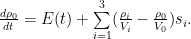
So this post will flesh the answer out by observing that the response defined by the “Bern TAR” parameters is simply the solution to the following equation:

where

But that equation describes the system that the accompanying diagram depicts. And that system does not impose partitioning of the type that the above-cited post describes.

In the depicted system, four vessels of respective fixed volumes 


Additionally, a gas source can add gas to the first vessel at a rate 

If appropriate selections are made for the 
The gas represents carbon (typically as a constituent of carbon dioxide, cellulose, etc.), the first vessel represents the atmosphere, the other vessels represent other parts of the carbon cycle, the membranes represent processes such as photosynthesis, absorption, and respiration, and the stimulus 
I digress here to draw attention to the fact that I’ve just moved the pea. The flow from the source does not represent all emissions, or even all anthropogenic emissions. It represents the flow only of carbon that had previously been sequestered for geological periods as, e.g., coal, and that is now being returned to the cycle of life. Thus re-defining the model’s emissions quantity finesses the objection some have made that the Bern Model requires either that processes (implausibly) distinguish between anthropogenic and natural carbon-dioxide molecules or that atmospheric carbon dioxide increase without limit.
Now, there’s a lot to criticize about the Bern Model; many of the criticisms can be found in the reader comments that followed the partitioning-argument post. Notable among those were richardscourtney’s . Also persuasive to me was Dr. Brown’s observation that the atmosphere holds too small a portion of the total carbon-cycle content for the 0.152 value assigned to the infinite-time-constant component to be correct. And much in Ferdinand Engelbeen’s oeuvre is no doubt relevant to the issue.
As the diagram shows, though, the left, atmosphere-representing vessel receives all the emissions, and it permits all of the other vessels to compete freely for its contents according to their respective membranes’ permeabilities. So what is not wrong with the model is that it requires the atmosphere to partition its contents, i.e., to withhold some of its contents from the faster processes so that the slower ones get the share that the model dictates.
Related articles
- On CO2 residence times: The chicken or the egg? (wattsupwiththat.com)
So what is not wrong with the model is that it requires the atmosphere to partition its contents, i.e., to withhold some of its contents from the faster processes so that the slower ones get the share that the model dictates.
+++++++++++
The problem I see is that every year the earth absorbs 1/2 of human emissions, and this amount is dependent upon human emissions, not total CO2 is the system, as this has been going on for many years.
now it is true that human beings have an infinite capacity to rationalize, so I’m sure there are as many different explanations for this are there are people. And every expert will have 2 explanations. However, to me it is a nonsense.
How can nature tell how much CO2 humans are producing each year, such that nature absorbs almost exactly 1/2 year of human emissions after year after year? How come nature doesn’t absorb the excess as a function of the total? How can nature separate human emissions from natural emissions?
This to me is the crux of the problem. Nature cannot tell human from natural emissions and thus what we observe is not what we believe it to be. The 1/2 figure has mislead us into believing facts not yet in evidence. the unknown is staring us in the face.
Nick Stokes: “The model is empirical. It’s true that we don’t have long enough observation to accurately measure a 171 year time number. ”
You do understand that the second sentence refutes the first sentence, right? If it is not based on observation — it is not empirical. Unless you want to wordsnitch the definition of ’empirical’ to be the same as ‘unempirical.’
tty: “However I have no explanation why oceanic outgassing would lag rising temperature less than accumulation lags sinking temperatures.”
How about this? Ocean outgassing in warm tropical and subtropical upwelling zones is intercepted more efficiently by microbial dark matter than in the polar downwelling brine rejection zones at -2C.
Greg Goodman says: December 2, 2013 at 12:45 pm
Sorry Greg – I do not accept your comments, and I do not want to pursue this discussion further.
If you want to critique, you have to first demonstrate that you understand what was said, and what was not said.
Allan MacRae says: “Sorry Greg – I do not accept your comments, and I do not want to pursue this discussion further.”
Allan, that is a very poor response to anything. if you want to refuse to accept my comments you need to first demonstrate that you have understood what they said.
I am in total agreement with the 9month lag and what it tells us about phase relationship. I have posted similar stuff myself and am working on something much more detailed which goes further. My comment here was merely that you are using a crap filter and your results may be clearer if you used a better one. (See my article on Judth Curry’s site for a detailed analysis and some ready made alternatives , with code !)
If you don’t think that running means distort data and are probably reducing the correlation that you are trying to demonstrate, please post a comment on Climate Etc. thread.
If you think I am criticising your article more than that you are mistaken. The dominant periodicity once the annual and sub-annual variation is removed is about 3 years, this is 4x9months thus the two are in quadrature.
Here is the clear alignment of dCO2 and SST using a lanczos filter.
http://climategrog.wordpress.com/?attachment_id=720
You will notice that the correlation is not so great in the detail beyond 2000. However, there is a remarkable correlation with a variable delay on Arctic Oscillation.
http://climategrog.wordpress.com/?attachment_id=259
Conclusion is that it is not trivially SST but it does account for a large amount of the variation.
PS. As Salby points out in his lecture, geological records show temp and CO2 correlate directly but with a substantial lag. That raises the question : on what time-scale does it flip from derivative to direct correlation?
I have an answer to that question that I am currently writing up and it is a little surprising.
jorgekafkazar says:
December 2, 2013 at 9:22 am
Or is it dominated by the larger Southern Hemisphere (“SH”) oceanic surface area?
It is easy to make the distinction: ocean CO2 releases are slightly increasing the δ13C level of the atmosphere, while CO2 releases from vegetation are firmly decreasing the δ13C level. Uptake by the oceans also slightly increases the δ13C level (because both ways are pure physical partitioning where the lightest isotope gets faster in/out, but the ocean surface is much higher in δ13C level than the atmosphere), while the uptake by plants (no matter C3 or C4) firmly increases the δ13C level. That gives in average for the past 22 years (CO2 and δ13C zeroed in January) :
http://www.ferdinand-engelbeen.be/klimaat/klim_img/seasonal_CO2_d13C_MLO_BRW.jpg
which shows that the variability over the seasons is completely dominated by the NH vegetation.
The trend also comes from the NH, as can be seen by comparing the trends over the years for different stations:
http://www.ferdinand-engelbeen.be/klimaat/klim_img/co2_trends_1995_2004.jpg
It takes time for the increase to reach altitudes and to pass the ITCZ from the NH to the SH.
Vegetation is not the cause of the increase, as the oxygen balance shows a small deficit, caused by increased growth.
The oceans are not the cause, as the most important upwelling places are in the SH equatorial Pacific, but the increase is in the NH first (and the δ13C trend is opposite to ocean releases).
Other possible natural sources are either too small or too slow…
So what is left?
“So what is left?”
Never the most convincing argument.
Your plot of relative timing is interesting.
http://www.ferdinand-engelbeen.be/klimaat/klim_img/co2_trends_1995_2004.jpg
Following your simple logic that this is the progression of the same signal (impossible to see in the integrated levels), it suggests that the increase starts in the Arctic , as indicated by Barrow station in Alaska.
Compare to my graph of d/dtCO2 (which does allow us to identify patterns) :
http://climategrog.wordpress.com/?attachment_id=259
It shows Arctic atm. pressure correlates with a strong lead.
Joe Born says:
In this case equilibrium is equal molar concentrations. There are no chemical effects biasing the system. The partial pressure (in the case, the complete pressure) is proportional to the molar concentration and is, as I indicated above, rho / V.
Sorry, a bit late in the discussion, as I was travelling…
There are huge chemical effects biasing the system, that is one of the basics of the Bern model. The three main sinks: ocean surface, deep oceans and vegetation all three are assumed to react with their own time constants, but also limitations in maximum uptake.
For the fastest, the ocean mixed layer, that is anyway certain: a 100% change in the atmosphere is followed by a 100% change of free CO2 in the ocean surface, as per Henry’s law, but as free CO2 in the ocean surface is only 1% of total carbon, the total carbon increases with ~10%, thanks to the chemical equilibria: 10 times more than for fresh water, but 10 times less than the change in the atmosphere.
That is the Revelle (or buffer) factor. Chemical equilibria explained in:
http://www.eng.warwick.ac.uk/staff/gpk/Teaching-undergrad/es427/Exam%200405%20Revision/Ocean-chemistry.pdf
Thus the Bern model assumes that the ocean surface rapidely is in equilibrium, but limited in capacity (I assume that the 19% is including the fast part of the biosphere besides the ocean surface). Which is theoretically and empirically proven. DIC (total inorganic carbon) increased about 10% of the atmospheric increase over the past decades as measured in Bermuda and Hawaii:
http://www.biogeosciences.net/9/2509/2012/bg-9-2509-2012.pdf
http://www.pnas.org/content/106/30/12235.full.pdf
The same for the deep oceans, but the deep oceans don’t show any sign of saturation, at least not for the foreseeable future, as the pCO2 of the cold sinking places is and remains very low, thus still increasing their uptake for increasing CO2 levels in the atmosphere. The Revelle factor isn’t applicable for non-surface waters under high pressure.
The same for vegetation: there is no saturation limit for more permanent storage of carbon in soils. After all that is what we are burning as coal nowadays…
Curiously, the fact that 60% of the anthropogenic CO2 emissions ‘disappears’ into some mysterious sink is not reflected in the Bern equation. i.e. It does not take a 171 years for 60% of the anthropogenic CO2 emissions to disappear every year.
It should be noted that we are busy cutting down rainforest to grow food to converted to biofuel and in the Amazon in addition cutting down rainforest to convert to pasture, so there is a significant which causes a reduction in carbon sinks and an increase in carbon emission. Calculations of AF therefore need to include the land conversion in addition to ‘fossil’ fuel consumption.
In an attempt to avoid an embarrassing reduction in the fraction of the CO2 that remains in the atmosphere, the amount of CO2 that is emitted due to the conversion of rainforest to agricultural land has been steadily reduced.
Carbon cycle modelling and the residence time of natural and anthropogenic atmospheric CO2: on the construction of the “Greenhouse Effect Global Warming” dogma. By Tom V. Segalstad
http://folk.uio.no/tomvs/esef/ESEF3VO2.pdf
http://radioviceonline.com/wp-content/uploads/2009/11/knorr2009_co2_sequestration.pdf
“Is the airborne fraction of anthropogenic CO2 emissions increasing?
(William: See Humlum et al for the other paradox.)
Several recent studies have highlighted the possibility that the oceans and terrestrial ecosystems have started losing part of their ability to sequester a large proportion of the anthropogenic CO2 emissions. This is an important claim, because so far only about 40% of those emissions have stayed in the atmosphere, which has prevented additional climate change. This study re-examines the available atmospheric CO2 and emissions data including their uncertainties. It is shown that with those uncertainties, the trend in the airborne fraction since 1850 has been 0.7 ± 1.4% per decade, i.e. close to and not significantly different from zero. The analysis further shows that the statistical model of a constant airborne fraction agrees best with the available data if emissions from land use change are scaled down to 82% or less of their original estimates. Despite the predictions of coupled climate-carbon cycle models, no trend in the airborne fraction can be found.
Of the current 10 billion tons of carbon (GtC) emitted annually as CO2 into the atmosphere by human activities [Boden et al., 2009; Houghton, 2008], only around 40% [Jones and Cox, 2005] remain in the atmosphere, while the rest is absorbed by the oceans and the land biota to about equal proportions [Bopp et al., 2002]. This airborne fraction of anthropogenic CO2 (AF) is known to have stayed remarkably constant over the past five decades [Jones and Cox, 2005], but if it were to increase in a way predicted by models, this could add another 500 ppm of CO2 to the atmosphere by 2100 [Friedlingstein et al., 2006], significantly more than the current total.
Conclusion
[25] From what we understand about the underlying processes, uptake of atmospheric CO2 should react not to a change in emissions, but to a change in concentrations. A further analysis of the likely contributing processes is necessary in order to establish the reasons for a near-constant AF since the start of industrialization. The hypothesis of a recent or secular trend in the AF cannot be supported on the basis of the available data and its accuracy.”
Ferdi, you will recall you convinced me about the dilution argument that Gosta Pettersson claims you “fooled” on. Well I think there is clear evidence of this happening in the Nordkap data.
http://climategrog.wordpress.com/?attachment_id=723
It shows a fairly rapid decay, so this should inform us about turnover time and the relative amplitude of the fast response and deeper time constant.
The initial annual swing on C14 is about 10% peak to peak and it’s gone in 10 years.
It may be jumping the gun to attribute this all to oceanic reaction but there is a fast response in climate that will equilibrate in under a decade. I have other evidence of this happening.
It seems to account for about 20% of the atmospheric change.
oops: … claims you ME “fooled” on.
It appears the Bern equation was created to justify CAWG, as a means to an end. As noted below as suspended organic solids sink to the bottom of the ocean in less than a year we do not wait more than a 1000 years for anthropogenic CO2 to disappear into the deep ocean.
Also it is interesting that fraction of anthropogenic CO2 that remains in the atmosphere has decreased from roughly 50% at the time Segalstad wrote this brief to 40%.
Carbon cycle modeling and the residence time of natural and anthropogenic atmospheric CO2: on the construction of the “Greenhouse Effect Global Warming” dogma. By Tom V. Segalstad
http://folk.uio.no/tomvs/esef/ESEF3VO2.pdf
“At this point one should note that the ocean is composed of more than its 75 m thick
top layer and its deep, and that it indeed contains organics. The residence time of
suspended POC (particular organic carbon; carbon pool of about 1000 giga-tonnes;
some 130% of the atmospheric carbon pool) in the deep sea is only 5-10 years. This
alone would consume all possible man-made CO2 from the total fossil fuel reservoir
(some 7200 giga-tonnes) if burned during the next 300 years, because this covers 6
to 15 turnovers of the upper-ocean pool of POC, based on radiocarbon (carbon-14)
studies (Toggweiler, 1990; Druffel & Williams, 1990; see also Jaworowski et al.,
1992 a). The alleged long lifetime of 500 years for carbon diffusing to the deep ocean
is of no relevance to the debate on the fate of anthropogenic CO2 and the “Greenhouse
Effect”, because POC can sink to the bottom of the ocean in less than a year
(Toggweiler, 1990).
7. Boost for the dogma – the evasion “buffer” factor
Bacastow & Keeling (1973) elaborate further on Bolin & Eriksson’s ocean “buffer”
factor, calling it an “evasion factor” (also called the “Revelle factor”; Keeling &
Bacastow, 1977), because the “buffer” factor is not related to a buffer in the chemical
sense. A real buffer can namely be defined as a reaction system which modifies or
controls the value of an intensive (i.e. mass independent) thermodynamic variable
(pressure, temperature, concentration, pH, etc.). The carbonate system in the sea will
act as a pH buffer, by the presence of a weak acid (H2CO3) and a salt of the acid
(CaCO3). The concentration of CO2 (g) in the atmosphere and of Ca (aq) in the ocean 2+
will in the equilibrium Earth system also be buffered by the presence of CaCO3 at a
given temperature (Segalstad, 1996).”
If one is interested in the cartoon, mythological Bern model this is the summary that is continually repeated in this thread.
http://www.ocean.washington.edu/courses/oc400/sarmientogruber.pdf
Ferdinand Engelbeen:
Thank you very much for that summary and in particular for that first link, which I’ve already found helpful. I confess that, although I have found your contributions highly informative, I’ve been only a dilettante; it remains on my list even to digest the series you did here three years ago fully . But I like to think doing so is more than a velleity.
As to the specific question before the house, namely, whether the Bern mathematics requires partitioning of the type Mr. Eschenbach contended, my argument is that those real-world considerations are largely beside the point; if one can provide, as I have, a system to whose equations the first equation above provides the solution, then the Bern mathematics imposes no such requirement if that system doesn’t partition. And, as I said above, the left-hand vessel’s contents are all available to all the right-hand vessels.
But a question on which it only now occurs to me that the considerations you’ve laid out may bear is whether “since the atmosphere at 600 PgC represents only 1.5% of the active carbon sinks (38,000 PgC in the hydrosphere and 2000 PgC in the biosphere) only 1.5% of any excess CO2 we add to the atmosphere will remain indefinitely.” That is, can we conclude that the world-wide “equilibrium constant” (if one can apply that term to the results of so disparate a set of processes) inferred from the pre-industrial carbon distribution will ultimately re-establish itself after we’ve perturbed the system. As a previous comment indicates, I’m under the impression that it would, but I’m too far from conversant with the various factors to be entitled to an opinion.
ferdberple: “So what is not wrong with the model is that it requires the atmosphere to partition its contents, i.e., to withhold some of its contents from the faster processes so that the slower ones get the share that the model dictates.
+++++++++++
“The problem I see is that every year the earth absorbs 1/2 of human emissions, and this amount is dependent upon human emissions, not total CO2 is the system, as this has been going on for many years.”
Different explanations of the missing half of human emissions have been made by people more informed than me, but I’ll take this opportunity to put my two cents’ worth in. Although I haven’t identified any compelling mechanism, I speculated in the course of preparing the above diagram that there actually is a partitioning in the atmosphere–between the admissions whose effects we can measure and those we can’t. Specifically, if certain sources (utility boilers?) cause high, very localized concentrations that result in high, very localized uptake by a high-capacity sink, could that explain the preferential human-emissions’ uptake?
The problem probably lies in the naive _assumption_ that the increase is totally due to a residual of human emissions. Pettersson’s proposition is that outgassing accounts for about half the rise and that more than half of emissions are being absorbed. This would explain the huge discrepancy of the “missing sinks” and balance the carbon budget.
This seems more credible to me than negligible out-gassing _assumptions_ and missing sinks to add to the missing heat.
Pettersson’s third paper covers this and is still avavailable on his site htt://false-alarm.net
Allan MacRae says on December 2, 2013 at 8:57 am
Then there are other days when I think the MBA (Mass Balance Argument) is overly simplistic. The limited data I have seen suggests that even in urban environments where fossil fuels are locally combusted, the daily CO2 signature is overwhelmingly natural. It appears that CO2 is sufficiently scarce that plants quickly gobble up excess CO2 close to the source. Yum!
Joe Born says on December 3, 2013 at 3:17 am
Specifically, if certain sources (utility boilers?) cause high, very localized concentrations that result in high, very localized uptake by a high-capacity sink, could that explain the preferential human-emissions’ uptake?
Hi Joe,
Note the similarity in our comments.
The data I referred to is from Salt Lake City. Ii is interesting as winter sets in…
http://co2.utah.edu/index.php?site=2&id=0&img=32
Regards, Allan
Greg Goodman says on December 2, 2013 at 11:34 pm
Thank you for your clarification Greg.
I found your previous comments imprecise and impolite.
Are some filters better than others? – Yes.
Do allegedly better filters materially change my conclusions? – No.
Have there been any significant new scientific insights on this topic since my January 2008 icecap paper? – Not that I have seen, although my 2008 hypo has greater popularity.
I wish you good fortune is your scientific endeavours – there is much more to be discovered.
I suggest that in five-to-ten more years the following Conclusions will be widely accepted by reputable climate scientists.
Regards, Allan
http://wattsupwiththat.com/2013/11/21/on-co2-residence-times-the-chicken-or-the-egg/#comment-1488142
Conclusions:
The evidence from the modern data record AND the ice core record indicates that atmospheric CO2 does not primarily drive Earth’s temperature, and temperature primarily drives atmospheric CO2. This does not preclude the Mass Balance Argument being correct, but its relevance to the “environmental catastrophe debate” (catastrophic global warming, etc.) is moot, because increased atmospheric CO2 has NO significant impact on temperature, and is beneficial to both plant and animal life. Claims that increased atmospheric CO2, from whatever source, causes dangerous runaway global warming, wilder weather, increased ocean acidification, and other such alarmist claims are NOT supported by the evidence.
The climate models cited by the IPCC fail because, at a minimum, these models employ a highly exaggerated estimate of climate sensitivity to increased atmospheric CO2. In fact, since Earth’s temperature drives atmospheric CO2 rather than the reverse, which is assumed by the IPCC-cited climate models, these models cannot function correctly. The IPCC-cited climate models also grossly under-estimate the magnitude of natural climate variation.
ferdberple.
You miss the point, yes absorbtion is related to the absolute level of CO2 in the atmosphere, but CO2 is increasing and with it so is the absorption. Both the rate of CO2 release AND the sinking rate increase together, the sinking rate being driven by the increase in CO2 partial pressure, temperature and fresh water availability all of which are supposed to be positively correlated with CO2. It has been shown that doubling CO2 increases plant mass some 30% or so, implying that the consumption rate increases by 1/3 of the change in the emission rate. At the same time secondary effects also occur due to temperature and water availability but also the density (number of plants per square meter) and the scope, plants growing in places where before they didn’t. This naturally applies to ocean biota too. The sinks expand as the level of CO2 rises, not as the rate of it rises.
This is a classic negative feedback, emission gives rise to increased CO2 which gives rise to increased sinking capacity, which opposes the emission causing the rise. There is obviously a lag, but if the lag is short enough, then sure, this mechanism is capable of taking up 50 or 60 % of the 3% delta CO2 intra year. The sinks dont need to know what the source is since they are only reacting to the increased level over the annual cycle.
Maybe your comment wasn’t directed at this process, if so forgive my interjection
Greg Goodman says:
December 3, 2013 at 12:48 am
The Barrow plot is a little misleading (but quite spectacular), as much of the air masses there are mixed with air from lower latitudes via the Ferrel cells. The CO2 levels from Schauinsland (Black Forest, South-West Germany) at 1200 m height even shows a larger seasonal amplitude than Barrow:
http://archiv.ub.uni-heidelberg.de/volltextserver/6870/1/SchmidtJGR2003.pdf
My impression is that the change over the seasons shifts with temperature from the mid-latitudes to the high North and that the North shows a mix of what happened more southward + what happens nearby, but later in the season.
Additional for 14C is that a huge part is directly absorbed but comes back in the next season with the fallen leaves, but that part is getting in more permanent storage + that the Nordkapp is practically in the middle of the largest sink place of the oceans.
If one is interested in the cartoon, mythological Bern model this is the summary that is continually repeated in this thread.
http://www.ocean.washington.edu/courses/oc400/sarmientogruber.pdf
Hmm, don’t like this document, this implies that sinks will not eventually expand to balance emission and that anthropogenic excess can never be fully balanced by nature but this is clearly wrong, while increasing the rate of CO2 such as to maintain a constant deficit between emission and absorbtion would do that, maintenance of a constant rate of emission will clearly produce a new equilibrium between emission and absorption at some partial pressure of CO2 and not lead to indefinitely increasing CO2 levels. If adaption occurs at a rate of 50 % of the imbalance per year as implied by the missing sinks, then 5 years is all it takes to come back to equilibrium by my math.
Joe,
Based on the text of the Bern model paper, I don’t believe that you are accurately representing their model or mathematics. For example, the authors have demonstrated an appreciation for the forward and reverse exchange rate constants being unique. Also, they did not derive a fourth-order differential equation from a system of first-order ODEs as you apparently have done. I cannot offer further critique of your mathematics without an explicit description of how you arrived at your fourth-order diff eq. I do not see how you introduced the higher order derivatives or why you didn’t solve the system of first-order ODEs using standard techniques.
The form of the Bern equation can correspond to a wide variety of compartment box models, including a box model as you have depicted. However, the Bern model does not require symmetry in the rate constants that you have assumed, as explained in their paper and also here: http://nvlpubs.nist.gov/nistpubs/jres/090/jresv90n6p525_A1b.pdf.
The Bern model states that the atmospheric CO2 concentration vs. time decay profile should be multi-phasic, which results from a coupled compartmental box system engaging in a “tug-of-war” as it strives to reach equilibrium. The different time constants of the Bern model actually represent different equilibration phases; more properly, the different decay rate constants correspond to the eigenvalues of the system and depend only on the individual rate constants. The “faster” time constants are a consequence of faster equilibriation phases overlapping with slower equilibration phases.
The real question is whether or not a multi-compartment box model is actually supported by actual data.
CO2 is described by a higher order equation and has naturally several time scales of decay. This is trivial. It is also trivial that the Bern model is in principle correct.
What is not trivial, are the particular values of all those constants in the Bern model.
Although the main constants are based on well known chemical processes, the only way to check whether they are applicable to the Earths atmosphere as a whole is to compare them with the experiment: how does CO2 in the atmosphere develop with time.
We have no sufficient data to check experimentally any factor in the Bern equation that contains a time scale longer than a couple decades.
Allan MacRae: “Note the similarity in our comments.”
Indeed. I had read your comment but failed to make the connection.
William Astley: “Curiously, the fact that 60% of the anthropogenic CO2 emissions ‘disappears’ into some mysterious sink is not reflected in the Bern equation. i.e. It does not take a 171 years for 60% of the anthropogenic CO2 emissions to disappear every year.”
That was the impression I had formed, too, but I didn’t try hard to confirm that it makes such an omission. I was tempted to “improve” the equation by taking that into account in formulating my diagram, but doing so in a half-way plausible manner would have made the equations uglier than they already are. (I spared everyone the derivations, but, believe me, they’re not pretty.)
Incidentally, thank you for the literature references and summaries. I wish I were well-versed enough in the related science critically to judge Segalstad’s work regarding the effects of deep-layer particulate organic carbon.