Guest essay by Joe Born
Is the Bern Model non-physical? Maybe, but not because it requires the atmosphere to partition its carbon content non-physically.
![bern_irf[1]](http://wattsupwiththat.files.wordpress.com/2013/12/bern_irf1.gif)
A Bern Model for the response of atmospheric carbon dioxide concentration 


![\rho_{CO_2}(t)=C_{CO2}\int\limits_{-\infty}^{t}E_{CO_2}(t')\left[ f_{CO_2,0}+\sum\limits_{S=1}^{n} f_{CO_2,S}e^{-\frac{t-t'}{\tau_{CO_2,S}}} \right]dt' .](https://s0.wp.com/latex.php?latex=%5Crho_%7BCO_2%7D%28t%29%3DC_%7BCO2%7D%5Cint%5Climits_%7B-%5Cinfty%7D%5E%7Bt%7DE_%7BCO_2%7D%28t%27%29%5Cleft%5B+f_%7BCO_2%2C0%7D%2B%5Csum%5Climits_%7BS%3D1%7D%5E%7Bn%7D+f_%7BCO_2%2CS%7De%5E%7B-%5Cfrac%7Bt-t%27%7D%7B%5Ctau_%7BCO_2%2CS%7D%7D%7D+%5Cright%5Ddt%27+.&bg=ffffff&fg=000&s=0&c=20201002)
The “Bern TAR” parameters thus adopted state that the carbon-dioxide-concentration increment 

where the 


There are a lot of valid reasons not to like what that equation says, the principal one, in my view, being that the emissions and concentration record we have is too short to enable us to infer such a long time constant. What may be less valid is what I’ll call the “partitioning” version of the argument that the Bern model is non-physical.
That version of the argument was the subject of “The Bern Model Puzzle.” According to that post, the Bern Model “says that the CO2 in the air is somehow partitioned, and that the different partitions are sequestered at different rates. . . . Why don’t the fast-acting sinks just soak up the excess CO2, leaving nothing for the long-term, slow-acting sinks? I mean, if some 13% of the CO2 excess is supposed to hang around in the atmosphere for 371.3 years . . . how do the fast-acting sinks know to not just absorb it before the slow sinks get to it?” (The 371.3 years came from another parameter set suggested for the Bern Model.)
The comments that followed that post included several by Robert Brown in which he advanced other grounds for considering the Bern Model non-physical. As to the partitioning argument, though, one of his comments actually came tantalizingly close to refuting it. Now, it’s not clear that doing so was his intention. And, in any event, he did not really lay out how the circuit he drew (almost) answered the partitioning argument.
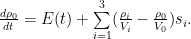
So this post will flesh the answer out by observing that the response defined by the “Bern TAR” parameters is simply the solution to the following equation:

where

But that equation describes the system that the accompanying diagram depicts. And that system does not impose partitioning of the type that the above-cited post describes.

In the depicted system, four vessels of respective fixed volumes 


Additionally, a gas source can add gas to the first vessel at a rate 

If appropriate selections are made for the 
The gas represents carbon (typically as a constituent of carbon dioxide, cellulose, etc.), the first vessel represents the atmosphere, the other vessels represent other parts of the carbon cycle, the membranes represent processes such as photosynthesis, absorption, and respiration, and the stimulus 
I digress here to draw attention to the fact that I’ve just moved the pea. The flow from the source does not represent all emissions, or even all anthropogenic emissions. It represents the flow only of carbon that had previously been sequestered for geological periods as, e.g., coal, and that is now being returned to the cycle of life. Thus re-defining the model’s emissions quantity finesses the objection some have made that the Bern Model requires either that processes (implausibly) distinguish between anthropogenic and natural carbon-dioxide molecules or that atmospheric carbon dioxide increase without limit.
Now, there’s a lot to criticize about the Bern Model; many of the criticisms can be found in the reader comments that followed the partitioning-argument post. Notable among those were richardscourtney’s . Also persuasive to me was Dr. Brown’s observation that the atmosphere holds too small a portion of the total carbon-cycle content for the 0.152 value assigned to the infinite-time-constant component to be correct. And much in Ferdinand Engelbeen’s oeuvre is no doubt relevant to the issue.
As the diagram shows, though, the left, atmosphere-representing vessel receives all the emissions, and it permits all of the other vessels to compete freely for its contents according to their respective membranes’ permeabilities. So what is not wrong with the model is that it requires the atmosphere to partition its contents, i.e., to withhold some of its contents from the faster processes so that the slower ones get the share that the model dictates.
Related articles
- On CO2 residence times: The chicken or the egg? (wattsupwiththat.com)
– – – – – – – –
And the BERN modelers explained that time constant how?
(a why question is pending)
John
Monckton of Brenchley: “I should be interested in comments on whether the Bern model’s value of 0.152 for the equilibrium constant is justifiably an order of magnitude greater than that which is derivable theoretically from the relative magnitudes of the contents of the atmosphere and of the active sinks,”
I haven’t done the math. In fact, I can’t put my hands on the data I’d need for the attempt. But my guess is that some fitting of the n = 3 version of the first equation above to the data could indeed spit out parameters like the Bern TAR numbers–or not. But my understanding of Willis Eschenbach’s work is that the magnitude of the residuals thereby obtained would not be much less than that which results from fitting to a single exponential decay.
Mr. Tol seems to be in possession of knowledge that would refute the conclusion thereby to be drawn, but so far on this thread he has hidden his light under a bushel.
Joe
I was really only answering the call by Dr Spencer to address tty’s comment.
The partitioning does seem a little peculiar and seems to assume some intelligence in the system. I think that the d13C signature may play a part though. If the atmosphere becomes enriched with 12C then biological uptake may be more rapid thus removing the extra CO2 (if depleted in 13C) more rapidly than say the inorganic processes. This then acts in a feedback loop until things stabilise? Perhaps this is the reason why they feel some partitioning is required.
Nick Stokes-
“Mathematically, a sum of exponentials is very hard to fit uniquely, because they are not at all orthogonal.”
Are you claiming that Fourier series are flawed? Surely not.
Perhaps the problem is not with a long term residual concentration, but the assumption that this residual has something to do with past history. The biosystem has its own central tendency whatever we or volcanoes do. To explain this requires an additional term in the model that is separate from the time dependent terms.
John Whitman: “And the BERN modelers explained that time constant how?”
I’m putting words in their mouths here, but I think they’d say they’re not trying to explain anything but rather saying that, if you want to treat the system as a black box characterized by a linear differential equation, what equation of order n + 1 would you come up with if you fitted it to the data.
One criticism of their result is given in my last response above to Lord M. It is based on work that I thought I remembered Willis Eschenbach’s having done, but I haven’t been able to locate that work again. (His post I referred to above isn’t it.)
I agree with Nick Stokes’ comment on the difficulty of fitting multiple exponentials to decay curves. They are classically ill-conditioned and may result in very large errors.
Since there is a considerable biological component in CO2 uptake and release, is this likely to be a linear process? (I realse that with the available data this might be impossible to establish).
cd says
” As part of the rock cycle volcanic input is balanced by subduction of carbonate minerals in rocks such as limestone at destructive continental plate margins; this produces the volcanoes. In short the volcanoes are returning the CO2 from the subducted rocks.”
Certainly, though some of the CO2 may also be from deep mantle sources, or entrained from carbonate rocks through which the magma rises. And the whole cycle: atmospheric CO2 -> oceanic CO2 -> marine organisms -> carbonate deposit on seabottom -> move to a subduction zone by plate tectonics -> subduct to a depth where magma forms -> magma rises to the surface -> magma degasses -> atmospheric CO2 probably takes a few hundred million years at the very least. And it is far from clear that it is a balanced process. Since atmospheric CO2 on the whole seems to have decreased during the Phanerozoic indications are that it is not.
Doc Martyn says:
“The 800 Ky ice core data shows that CO2 varies between 240-300 ppm during this period, so it is reasonable to conclude that some process mineralizes carbon rapidly when atmospheric CO2 is high and mineralizes it more slowly when atmospheric CO2 is low.”
Its more like 170-300 ppm, and since the concentration tracks the glacial cycles fairly closely, with some lag (short during deglaciations, much longer during glacier growth phases) it would seem that the oceans are the only sink that could vary fast enough (on a time-scale of a few millenia). However I have no explanation why oceanic outgassing would lag rising temperature less than accumulation lags sinking temperatures.
The phrase “bern model” prodded my mmeory of having read an article by Jarl Ahlbeck a decade or so ago where he put forward a chemical mass balance model for the uptake of carbon dioxide by the oceans and biosphere, and then used it to predict the a size of around 17 GtC/year CO2 ocean/biosphere sink when the magic double of 560 ppmV concetration of CO2 in the atmosphere would happen instead of 8.5 GtC/yr (fro, The Bern Model I assume). He did this a little before the millennial shift and therefore had had only acess to data up to the year 1997 available estimate his parameters, but it should be check If his model has been tracking reality since then, or if we are really living inside the big bear bottles the author says the IPCC-(bern???)model thinks.
The article can be found at this URL.
http://www.john-daly.com/co2-conc/ahl-co2.htm
Joe,


 .
.
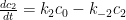
Your equations for the pressure in each box are incorrect given your compartment box model. This is a system of coupled first order linear differential equations that must be solved by an approach such as that described here: http://web.ist.utl.pt/berberan/data/40.pdf.
For the given system, an acceptable system of equations can written as follows (where c represents the molar concentration of the species of interest in the ith compartment):
subject to the chemical thermodynamic equilibrium constraint (i.e. equilibrium constant or partition coefficient relation):
Richard Tol:
George Box’s aphorism that “All models are wrong.” is obviously incorrect in reference to the natural laws. Until recently, it was correct in reference to models of complex systems such as the climate. Today, however, through the use of modern information theory, it is possible to build a model of a complex system that conforms to the principles of reasoning, thus not being wrong. All currently available climatological models are, however, wrong.
Fun stuff ladies and gentlemen.
Chaucer ably described the dominant factor in Earth`s carbon balance, as follows:
WHAN that Aprille with his shoures soote
The droghte of Marche hath perced to the roote,
And bathed every veyne in swich licour,
Of which vertu engendred is the flour…
We now have the benefit of the beautiful AIRS data animation of atmospheric CO2 at
http://svs.gsfc.nasa.gov/vis/a000000/a003500/a003562/carbonDioxideSequence2002_2008_at15fps.mp4
The CO2 seasonal sawtooth is dominated by the larger Northern Hemispheric (“NH“) landmass.
Atmospheric CO2 drops in NH Spring and Summer during Chaucer’s “shoures soote” as photosynthesis dominates, and then CO2 increases in NH Fall and Winter as oxidation becomes the dominating factor in this huge and wondrous equation.
The annual amplitude (from memory) of this magnificent seasonal CO2 sawtooth is about 16-18ppm in the far North (measured at Barrow AK), and as little as 1-2 ppm at the South Pole.
Nevertheless the average upward slope of the “global” (approx. equal to Mauna Loa) CO2 sawtooth is about 1-2 ppm per year. Aye, there`s the rub!
And some of us think we understand why CO2 increases (for example, the Mass Balance Argument attributes the CO2 increase to fossil fuel combustion), while Richard Courtney ably suggests that we don`t really know. I`m generally with Richard on this, although I wobble.
There are days when I think the Mass Balance Argument (`MBA`) has validity, although I suggest that other factors such as deforestation etc. may play a larger role, and it is not just fossil fuels.
Then there are other days when I think the MBA is overly simplistic. The limited data I have seen suggests that even in urban environments where fossil fuels are locally combusted, the daily CO2 signature is overwhelmingly natural. It appears that CO2 is sufficiently scarce that plants quickly gobble up excess CO2 close to the source. Yum!
In any case, the global CO2 Balance question is very interesting, but I suggest it is not that relevant to the oft-fractious global warming debate – because CO2 in Earth`s natural system is clearly driven by temperature and is at most an insignificant driver of temperature.
Some people insist that these matters must be quantified, so I will accommodate them:
The impact of the current increase in atmospheric CO2 on Earth temperature is less than one Standard Farticane*.
Regards to all, Allan
******
* 1 Standard Farticane = I Fart in a Hurricane, at Standard Temperature and Pressure.
CD:
“As part of the rock cycle volcanic input is balanced by subduction of carbonate minerals in rocks such as limestone at destructive continental plate margins; this produces the volcanoes. In short the volcanoes are returning the CO2 from the subducted rocks.”
<<<<<<<<<<<<<<<<<<>>>>>>>>>>>>>>>>>>
Not all volcanoes return subducted material. Some occur at spreading centers, others at “hot spots”, i.e., Hawaian Islands, and such do not return subducted material but tap directly into the mantle. So carbon is not being recycled but added to the crust or atmosphere, insofar as such volcanoes produce CO2. However, subducted material is recycled by those volcanoes that occur on the margins of subduction zones, as you say.
rtj1211 says: “I’m assuming of course that no-one will let you go and realise a load of carbon-14-labelled gas into the atmosphere right now……..”
Good news! Iran intends to go ahead with this experiment within the next ten years.
Allan MacRae says: “The CO2 seasonal sawtooth is dominated by the larger Northern Hemispheric (“NH“) landmass.”
Or is it dominated by the larger Southern Hemisphere (“SH”) oceanic surface area?
ZP: “Your equations for the pressure in each box are incorrect given your compartment box model. ”
Could you be a little more specific? The equations you wrote are not inconsistent with mine, except E in my system is a rate of mass flow, so I would have put E in your equations instead of dE/dt. Also, for parallelism I perhaps confusingly use rho to represent the mass (number of moles) in the vessels; it’s not a concentration. Other than that, your k’s are my S/V’s.
In short, you’ve told me the equations are wrong, but you haven’t pointed out where. I’d love to have someone vet my sums, but I’ll need a little more specificity if it is to do me any good.
DocMartyn: “Your three box model also ignores the fact that to interrogate the deep ocean, atmospheric CO2 must first interact with the surface layer; there is no direct route.”
That’s incorrect. There is significant up-welling of deep waters in certain ocean regions, esp. Indian Ocean and sinks at the poles. This is part of the thermohaline circulation. That provides a direct connection.
http://climategrog.wordpress.com/?attachment_id=715
The point you try to make may well apply to mid-ocean waters between the surface mixed layer and the thermocline.
I am writing up something that shows that the well-mixed layer has a time constant close to one year and equilibrates in under a decade with a change of the order of 10ppmv/K. The circa 15y ( Bern 18.6y ) time constant is presumably this mid level diffusion.
Lance Wallace fitted a time const of 1.17 years to Nordrap C14 data in an earlier discussion. This is close to what I’m finding by totally different methods that does not suffer from the lack of uniqueness described here for exponentials.
Gosta Pettersson is close to being correct in his conclusions but I think his working is wrong. He sees no need for the short period which IMO he should be applying to his El Nino changes.
He has recently pulled his papers 1 & 2 which he is rewriting them, so it will be interesting to see how he changes them.
me says: “with a change of the order of 10ppmv/K.”
That is atm 10ppmv. I view of the volume ratio, I would guess about 4x that for the mid-level reservoir giving total all the order of 50 ppmv/K. This is in rough agreement with Gosta’s figures by via a different (incompatible) calculation.
The resulting conclusion is the same w.r.t. solving the “missing sinks” issue: like the missing heat, it does not exist.
The k’s in the equations represent the specific rate constants governing the compartmental exchange rates. Your equations incorrectly assume that the forward rate constant ( ) is equal to the reverse rate constant (
 ), which allowed you to factor them out as a single constant S. There is no physical basis on which to assume that the forward rate constant should be equal to the reverse rate constant. And, the values will only be the same in the case where the equilibrium constant is unitary.
regarding the comment by tty:
Since the late Eocene, the world has cooled considerably which must mean cooler oceans and a greater capacity for holding CO2, presumably. But, in terms of geologic time, the carbon equation must be incalculable.
For example, carbonates are precipitated directly from ocean waters at such places as the Bahamas or the Yucatan shelf, such areas being known as carbonate platforms. Thus carbon is removed on a semi-permanent basis at such places. An ocean richer in CO2 would positively affect the rate of precipitation, presumably. I doubt that all these factors can be untangled.
jorgekafkazar says:
Allan MacRae says: “The CO2 seasonal sawtooth is dominated by the larger Northern Hemispheric (“NH“) landmass.”
Or is it dominated by the larger Southern Hemisphere (“SH”) oceanic surface area?
Yes, indeed. Yet another urban climatology assumption I guess.
Annual ‘saw tooth’ works out rather nicely actually since it can be modelled by two ramps or 12moand 6mo cosines (the latter being more physically real, but the first is handy for getting flow rates).
http://climategrog.wordpress.com/?attachment_id=721
The Bern model can be thought of as a partition of reservoirs, but that is only an approximation. Generally, such “long tailed” models arise from partial differential diffusion equations. The sum of exponentials is an expansion of eigenfunctions of the partial differential equation.
So, the place to begin is the PDE model, the equations and their boundary conditions, assumed by the Bern model.
Subduction is not required. Folding deposits deep enough for metamorphosis is sufficient to release CO2.
The CO2 sources for many of the ‘hot spot’ volcanoes, e.g., Hawaii, are unknown. Guesses about magma absorbing CO2 from sediments as magma passing through are just that, guesses.
Deep, really deep magmatic CO2 sources, are currently beyond our ken. CO2 out gassing from these hot spots may include primal CO2 still leaking from earth’ s core. Carbon content in metals often resides in carbides; oxygen in many forms, oxides to be simple. Bluntly speaking, carbon is abundant cosmically.
ZP: “here is no physical basis on which to assume that the forward rate constant should be equal to the reverse rate constant.”
If you’re talking about the real world, in which various factors affect “natural” emission (leftward flow) and uptake (rightward flow), I agree, and to that extent the model does not reflect reality.
If you’re talking about the model world, in which a permeable membrane conducts net flow in accordance with the pressure difference–i.e., with the difference in moles/unit volume, then I’m free to assume that a pressure on one side causes the same flow as the same pressure on the other.
The concept of equilibrium constant may be causing the difficulty here. Note that the process so drives flows that vessel contents tend toward proportionality with their volumes V. That’s where the equilibrium constants come from.