Guest essay by Joe Born
Is the Bern Model non-physical? Maybe, but not because it requires the atmosphere to partition its carbon content non-physically.
![bern_irf[1]](http://wattsupwiththat.files.wordpress.com/2013/12/bern_irf1.gif)
A Bern Model for the response of atmospheric carbon dioxide concentration 


![\rho_{CO_2}(t)=C_{CO2}\int\limits_{-\infty}^{t}E_{CO_2}(t')\left[ f_{CO_2,0}+\sum\limits_{S=1}^{n} f_{CO_2,S}e^{-\frac{t-t'}{\tau_{CO_2,S}}} \right]dt' .](https://s0.wp.com/latex.php?latex=%5Crho_%7BCO_2%7D%28t%29%3DC_%7BCO2%7D%5Cint%5Climits_%7B-%5Cinfty%7D%5E%7Bt%7DE_%7BCO_2%7D%28t%27%29%5Cleft%5B+f_%7BCO_2%2C0%7D%2B%5Csum%5Climits_%7BS%3D1%7D%5E%7Bn%7D+f_%7BCO_2%2CS%7De%5E%7B-%5Cfrac%7Bt-t%27%7D%7B%5Ctau_%7BCO_2%2CS%7D%7D%7D+%5Cright%5Ddt%27+.&bg=ffffff&fg=000&s=0&c=20201002)
The “Bern TAR” parameters thus adopted state that the carbon-dioxide-concentration increment 

where the 


There are a lot of valid reasons not to like what that equation says, the principal one, in my view, being that the emissions and concentration record we have is too short to enable us to infer such a long time constant. What may be less valid is what I’ll call the “partitioning” version of the argument that the Bern model is non-physical.
That version of the argument was the subject of “The Bern Model Puzzle.” According to that post, the Bern Model “says that the CO2 in the air is somehow partitioned, and that the different partitions are sequestered at different rates. . . . Why don’t the fast-acting sinks just soak up the excess CO2, leaving nothing for the long-term, slow-acting sinks? I mean, if some 13% of the CO2 excess is supposed to hang around in the atmosphere for 371.3 years . . . how do the fast-acting sinks know to not just absorb it before the slow sinks get to it?” (The 371.3 years came from another parameter set suggested for the Bern Model.)
The comments that followed that post included several by Robert Brown in which he advanced other grounds for considering the Bern Model non-physical. As to the partitioning argument, though, one of his comments actually came tantalizingly close to refuting it. Now, it’s not clear that doing so was his intention. And, in any event, he did not really lay out how the circuit he drew (almost) answered the partitioning argument.
So this post will flesh the answer out by observing that the response defined by the “Bern TAR” parameters is simply the solution to the following equation:

where

But that equation describes the system that the accompanying diagram depicts. And that system does not impose partitioning of the type that the above-cited post describes.

In the depicted system, four vessels of respective fixed volumes 


Additionally, a gas source can add gas to the first vessel at a rate 

If appropriate selections are made for the 
The gas represents carbon (typically as a constituent of carbon dioxide, cellulose, etc.), the first vessel represents the atmosphere, the other vessels represent other parts of the carbon cycle, the membranes represent processes such as photosynthesis, absorption, and respiration, and the stimulus 
I digress here to draw attention to the fact that I’ve just moved the pea. The flow from the source does not represent all emissions, or even all anthropogenic emissions. It represents the flow only of carbon that had previously been sequestered for geological periods as, e.g., coal, and that is now being returned to the cycle of life. Thus re-defining the model’s emissions quantity finesses the objection some have made that the Bern Model requires either that processes (implausibly) distinguish between anthropogenic and natural carbon-dioxide molecules or that atmospheric carbon dioxide increase without limit.
Now, there’s a lot to criticize about the Bern Model; many of the criticisms can be found in the reader comments that followed the partitioning-argument post. Notable among those were richardscourtney’s . Also persuasive to me was Dr. Brown’s observation that the atmosphere holds too small a portion of the total carbon-cycle content for the 0.152 value assigned to the infinite-time-constant component to be correct. And much in Ferdinand Engelbeen’s oeuvre is no doubt relevant to the issue.
As the diagram shows, though, the left, atmosphere-representing vessel receives all the emissions, and it permits all of the other vessels to compete freely for its contents according to their respective membranes’ permeabilities. So what is not wrong with the model is that it requires the atmosphere to partition its contents, i.e., to withhold some of its contents from the faster processes so that the slower ones get the share that the model dictates.
Related articles
- On CO2 residence times: The chicken or the egg? (wattsupwiththat.com)
Surely if you want to model carbon dioxide properly you should identify the possible fates of it and develop equations which mirror those possible fate processes?
So, you have to suggest the following fates of newly emitted carbon dioxide:
1. Absorption into the oceans (affected by the oceanic temperature and the steady state phytoplankton population, as well as an minerals rate-limiting for phytoplankton growth (if any are indeed limiting)).
2. Absorption by land-based plants and photosynthesising micro-organisms (affected by the air temperature, the sunshine hours and the overall density of photosynthetic factories within land-based plants etc).
3. Absorption into rain and snow with subsequent deposition into soil, rivers or snow.
4. No fate at all.
The other question to consider is where the carbon dioxide gets emitted (human/animal-related emissions will be pretty much at land level, wild fires may see heat driving the gas up to greater altitudes, whereas volcanic eruptions may emit it a few miles into the sky) and whether that affects the rate of that carbon dioxide’s fate into one of those four pathways (dependent on atmospheric/stratospheric/tropospheric mixing to equilibrium).
Fancy maths is all very well, but a model which is related to real earth processes is likely to produce a better prognostic model than one which happens to fit past data for no reason better than mathematical chance.
I don’t know if it is possible to monitor carbon dioxide fate safely using methods distinct from radioisotope labelling, but if people want to understand the kinetics of carbon dioxide fate, they are going to need to develop just such methods in order to succeed in their mission. I’m assuming of course that no-one will let you go and realise a load of carbon-14-labelled gas into the atmosphere right now……..
All models are wrong. Some are useful. The carbon cycle equation in the Bern model is a mathematical approximation of a very complex progress. This approximation was first published in 1988 by Ernst Maier-Reimer and Klaus Hasselmann. It is used in many simple climate models.
The question is not whether it is a physical representation. It is not, and nobody in their right mind ever claimed it was. The question is whether it is a good approximation. It is, unless you want to explore the very distant future or very extreme scenarios. The definitive work on this is by Georg Hooss, who tried his best to break the model but could not.
Forgive my LaTeX blunder. The second equation should read .
.
Professors Pettersson, supported to some extent by Professor Brown, maintains that since the atmosphere at 600 PgC represents only 1.5% of the active carbon sinks (38,000 PgC in the hydroisphere and 2000 PgC in the biosphere) only 1.5% of any excess CO2 we add to the atmosphere will remain indefinitely.
The Bern model’s value for alpha-zero, on that analysis, is overstated by an order of magnitude,
with the implication that the later points on the curve, in particular, show too slow a rate of decay, leaving more excess CO2 lingering in the atmosphere to cause warming than is correct.
As I explained in my posting on this, it is in the equilibrium constant – the excess remaining indefinitely resident in the atmosphere – that the chief difference between the Bern model and the bomb-test curve is to be found. The thread unfortunately became derailed by those who wanted to argue about semantic definitions of relaxation and adjustment times – not the main point..
The bomb-test curve shows a decay towards the equilibrium constant 0.015 derived by Professor Pettersson from values for the contents of the atmosphere and of the active sinks given by IPCC (2007, 2013). It would be interesting if, on this thread, the semantic quibblers were to exercise a self-denying ordinance, for I should be interested in comments on whether the Bern model’s value of 0.152 for the equilibrium constant is justifiably an order of magnitude greater than that which is derivable theoretically from the relative magnitudes of the contents of the atmosphere and of the active sinks, and empirically from the bomb-test curve.
I only ask because I want to know. As a curious layman, I do not know which position is correct. But the discrepancy is large, potentially influential in climate terms and, therefore, interesting.
Richard,
What do you define as the very distant future? Is it 5 years, 50 years or 500 years or more?
What most non-chemists are either forgetting or not mentioning for non-scientific reasons is the Dalton’s law going back to 1800s where the total pressure of air is:
P(air) = P(N2) + P(O2) + P(CO2) + …..
Since contribution from N2 and O2 is 99% and from CO2 only 0.04% it means that out of 2500 molecules that contribute towards any property of air, only 1 molecule comes from CO2. So, whenever is someone arguing what 1 molecule of CO2 is doing, one has to explain what are 2500 molecules of N2 and O2 surrounding that molecule of CO2 doing at the same time!
Richard Tol: “The definitive work on this is by Georg Hooss, who tried his best to break the model but could not.”
Could you provide us a link and explain how his work supports, for instance, the high magnitudes for the infinite- and long-time constant components of the TAR impulse response?
Monckton of Brenchley: “Professors Pettersson, supported to some extent by Professor Brown, maintains that since the atmosphere at 600 PgC represents only 1.5% of the active carbon sinks (38,000 PgC in the hydroisphere and 2000 PgC in the biosphere) only 1.5% of any excess CO2 we add to the atmosphere will remain indefinitely.”
To this layman that reasoning makes sense and militates against the Bern TAR parameters. It probably should be mentioned, though, that Professor Pettersson’s equation is equivalent to the first Bern equation above if n = 1 and f_CO2_0 is 0.015.
@terry
500+ years
@Joe Kirklin
http://www.schoepfung-und-wandel.de/NICCS/docum/welcome.html
“So what is not wrong with the model is that it requires the atmosphere to partition its contents, i.e., to withhold some of its contents from the faster processes so that the slower ones get the share that the model dictates.”
I agree with that. I think a simpler way of putting it is that some sinks are layered. The slow ones fill not from the air, but from the sinks above.
The model is empirical. It’s true that we don’t have long enough observation to accurately measure a 171 year time number. But we can use that to describe the long term behaviour, acknowledging that a timestep of 160 years, with appropriate parameter, would probably also have done well. And the component said to remain indefinitely simply reflects time scales too long to estimate at all. As Richard Tol says, it’s a model that works within a prescribed range.
Mathematically, a sum of exponentials is very hard to fit uniquely, because they are not at all orthogonal. It is an ill-conditioned problem. But all that means is that the Bern model is just one of many that can describe the process.
The empirical data show that Ao, the proportion of CO2 that remains in the atmosphere indefinitely must be very slightly less than zero. “Slugs” of CO2 are continuously being injected into the atmosphere by volcanoes, but the trend in CO2 in the atmosphere has been inexorably downward for the last 35 million years.
tty makes an interesting point I’d like to see comments on.
tty says: December 2, 2013 at 3:19 am
“The empirical data show that Ao, the proportion of CO2 that remains in the atmosphere indefinitely…”
It isn’t the proportion that remains in air indefinitely. It’s the proportion that remains so long that we can’t, in our limited observation span, measure the decay rate. The Bern model doesn’t claim to work for millennia. Here is an article from the originators in which they quote an expected range of 1765-2300 AD.
In answer to Roy Spencer, one should have regard to the various timescales to which the word “indefinitely” is applied. In the Neoproterozoic era, 750 Ma ago (Roy is too young to remember), there was at least 30% CO2 in the atmosphere. The CO2 was taken up in the oceans first as dolomitic limestone, then as amagnesic limestone, then as gypsum. During this phase, the equilibrium constant was demonstrably negative..
Now we are down to Henry’s Law, to the calcifying organisms, and to the growing net primary productivity of plants. In today’s geological conditions, therefore, the equilibrium constant may well be positive: and, if Professor Pettersson is right that it is the ratio of the carbon content of the atmosphere to that of the active sinks in the hydrosphere and biosphere, it is indeed slightly positive.
One problem with Professor Pettersson’s definition of the equilibrium constant is that, contrary to the geological evidence that it was for many ages negative, it can never be negative, for there cannot be a negative quantity of CO2 in the atmosphere. Another problem is that when the atmospheric partial pressure of CO2 doubles, the equilibrium “constant” also doubles by definition, and does so on a timescale of as little as a century.
I am beginning to wonder whether we have the slightest idea what the equilibrium constant is under today’s conditions. One cannot be sure that it remains negative. Equally, one cannot be sure that it is positive, still less that it is as strongly positive as the Bern model pretends. In this as in many other respects, the models are assuming that which cannot yet be known. What a relief it is, then, that The Science Is Settled, and we need not look any further into these matters.
tty: “‘Slugs’ of CO2 are continuously being injected into the atmosphere by volcanoes, but the trend in CO2 in the atmosphere has been inexorably downward for the last 35 million years.”
According to the attempt I made above to make sense of the Bern Model, tty’s statement would be a correct characterization of volcanoes’ actions if they are indeed introducing into the carbon cycle some carbon that for eons has not been participating.
To include the decay of which tty speaks, one or more of the vessels in the above diagram would need to be provided a second membrane, through which the gas would be consigned to the exterior darkness. Those membranes’ permeabilities (flow conductances) would need to be exceedingly small, of course.
tty is right to a point.
tty, adding a slug of co2 all things being equal cant reduce CO2 but all things being equal, but you’d intuitively expect that after the slug, given the emission and uptake remain constant at the level before the slug, that the CO2 would return over time to some equilibrium about the same as before the slug were added.
Despite Lord Moncktons plea, this problem is stated wrongly and assumes that uptake is a fixed function of time – but it is not, it’s a variable function of time, temperature, and CO2 concentrations at the places of major sinking activity.
The Bern model may be correct but it represents only a fraction of the system, a very simple model with no dynamic reactivity. We know for a fact that slugs of CO2 do not leave a large residual because despite the biosphere emitting slugs of CO2 constantly, CO2 has been known to contract.
The bomb test shows the turnover of CO2 due to all causes dynamic and static is on average more than this, but still misses the point that the response to a slug of extra CO2 may be much faster than the average drawdown if photosynthesis grows quickly with CO2 concentration, that is, if the sinks are being rate limited by the low concentration of CO2, if the sinking of CO2 is rate limited, then it will be harder to push up concentration, since the negative feedback is large, and any excess is rapidly acted against by the system,
The bomb test curve gives the decay rate of sink operating at an average rate between maybe 320 PPM and 400 PPM but how have the sinks actually responded, to that increase, the difference between the Bern model and the Bomb test may well be that factor. So how does that extra sinking capacity play out if we were to stop producing extra CO2 IE keep CO2 emission constant. That would depend on the dynamics of the feedback system that is rate limiting the sinks, and I might add the random effects of temperature on the biosphere. One must also consider the possibility that random pertubations have a bias, since the atmosphere is clearly biassed to reducing CO2 then random temperature changes are likely to be biassed to reducing CO2 over the long term.
For example, temp rises, oceans outgas, photosynthesis takes up ocean emissions limiting final CO2 level, temps fall, CO2 absorbed by oceans, CO2 now lower than it began.
Richard Tol: Thank you for the link. I assume you meant the dissertation to which that page in turn linked, i.e., to http://www.schoepfung-und-wandel.de/NICCS/docum/mpi_examen_83.pdf?
As to the software to which you did link, I’m flattered by the implication that I may be able to comprehend the nonlinear-system responses to which it is directed, but I must confess to skepticism that I will be enlightened.
Perhaps you could provide an executive summary of how you think that work supports the significant long-time-constant residues that the Bern TAR parameters dictate for the (linear) Bern Model.
tty
If I understand your point then a0 term seems ludicrous. If true then this would suggest CO2 would rise indefinitely given “additional” CO2.
But this excludes fluxes in the carbon cycle. As Lord Monckton has alluded to. Geochemical sequestration happens all the time via biological activity => carbonate minerals (for clarity this excludes sulphates such as gypsum which often precipitate in the same environment). As part of the rock cycle volcanic input is balanced by subduction of carbonate minerals in rocks such as limestone at destructive continental plate margins; this produces the volcanoes. In short the volcanoes are returning the CO2 from the subducted rocks. Interestingly, the d13 signature may vary from volcanos depending on whether the subducted rocks are biogenic or chemical in origin.
Lord M
One more appeal, let me use an electrical analogy, the bomb test gives us a hint as to the rate of sinking of energy. For an amplifier it’s akin to the average power sunk in the load. But does the power sunk in the load due to the dc biasing of the amplifier, give us any information about the gain of the amplifier? A small change in the conditions, may lead to a great change in output or a small one depending on the feedback acting. What are the feedback assumptiins in the bern model?
Instead of focussing on averaging a rate of sinking, I think we also need to use the bomb test to infer how the sinking rate has changed between the 1960s and now.
bobl: “We know for a fact that slugs of CO2 do not leave a large residual because despite the biosphere emitting slugs of CO2 constantly, CO2 has been known to contract”
In the diagram above, the CO2 emitted by the biosphere is represented by the leftward component of the net flow throw the membranes. Although this is something about which the model is silent, I would think of the net flow as a small difference between large leftward and rightward components. It is the sizes of those components–regarding which, again, the model is silent–that determines the rate of excess-carbon-14-concentration decay.
richardscourtney says: And the third model assumes that the carbon cycle is dominated by biological effects.
Looking at the annual changes in the amount of added CO2 to the atmosphere only this model makes sense.
It is worth noting that a large part of our emissions is absorbed by natural sinks. With this we agree everyone. From this it follows an important conclusion: natural sinks always react big increase on any new source. Natural sinks are not (almost) constants – there are (almost) in the balance with natural sources. The appearance of a new source always causes increase in productivity of sinks. Changes can not be linear.
How to react to organic of sinks – NPP, and decomposition (RH) on temperature changes?
Image 12 i 14 by M. Salby (http://wattsupwiththat.com/2013/11/22/excerpts-from-salbys-slide-show/) – here are the most important. They show – explained, that on the rapid changes in temperature RH reacts violently, and NPP (initially – and this is most important) responds slowly – much more slowly than RH. Land RH – respiration – responds rapidly to changes in temperature (rapidly – along with the temperature increase or decrease – much faster – more rapidly than NPP).
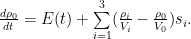
Therefore, I propose the following equation: “The Lotka–Volterra equations – models, also known as the predator–prey equations, are a pair of first-order, non-linear, differential equations frequently used to describe the dynamics of biological systems in which two species interact, one as a predator and the other as prey. The populations change through time according to the pair of equations”:
dx/dt = x (a -by)
dy/dt = – y (g-Sx)
where,
– x is the number of prey (for example, CO2 …);
– y is the number of some predator (for example, terrestrial plants …);
– dx/dt and dy/dt represent the growth rates of the two populations over time;
– t represents time; and
– a, b, g and S are parameters describing the interaction of the two, ie: where CO2 is the victim of a land photosynthesis is … predator.
Only by means of this equation we can prove that 4/5 – 5/6 (richardscourtney) added to the atmosphere of CO2 (presently) derived from natural sources. (http://climatechangescience.ornl.gov/content/historical-variations-terrestrial-biospheric-carbon-storage) : “Historical climatic variations which favored NPP over RH may have led to increased ecosystem carbon storage and might account for at least part of the “missing” sink required to balance the current century’s global carbon budget.”
When, however, the following: “NPP favored over RH”?
The higher density “prey” is easier, faster “hunting” …
Furthermore, according to the equation – model LV first grows RH, only when the NPP eg: produce seeds and produce new plants, it will be “favored NPP over RH” (http://en.wikipedia.org/wiki/File:Cheetah_Baboon_LV.jpg).
In the past it was. Sinks always coped with a much larger source of CO2. Never there have to saturation of sources. Always source increased.
Model Bern has a problem with sinks:
„It has been suggested that subtle and systematic changes in the net carbon fluxes as the result of climate variations or rising CO 2 concentrations over the past century may account for a substantial portion of the “missing” carbon sink of approximately 1 to 2 Gt C yr -1 needed to balance the contemporary atmospheric CO 2 budget.” (http://cdiac.esd.ornl.gov/pns/doers/doer34/doer34.htm)
NPP – in theory – be calculated as g C m-2 yr-1. Firstly, however, primarily calculated (or only) plant weight, and on this basis only estimated: g m-2 C-1 yr. In practice, not take into account the “nuances” such as: increase in CO2 = increase C concentration in plants: http://www.nature.com/scitable/knowledge/library/effects-of-rising-atmospheric-concentrations-of-carbon-13254108:
“The availability of additional photosynthate enables most plants to grow faster under elevated CO2, with dry matter production in FACE experiments being increased on average by 17% for the aboveground, and more than 30% for the belowground, portions of plants (Ainsworth & Long 2005; de Graaff et al. 2006). This increased growth is also reflected in the harvestable yield of crops, with wheat, rice and soybean all showing increases in yield of 12–14% under elevated CO2 in FACE experiments (Ainsworth 2008; Long et al. 2006).
Elevated CO2 also leads to changes in the chemical composition of plant tissues. Due to increased photosynthetic activity, leaf nonstructural carbohydrates (sugars and starches) per unit leaf area increase on average by 30–40% under FACE elevated CO2 (Ainsworth 2008; Ainsworth & Long 2005). Leaf nitrogen concentrations in plant tissues typically decrease in FACE under elevated CO2, with nitrogen per unit leaf mass decreasing on average by 13% (Ainsworth & Long 2005).”
Sorry by long quote…
Without a change in weight, the plants are able to accumulate many times more C than we think (and we are able to estimate by satellite). Tomatoes fertilized with CO2 – repeatedly increase the concentration of sugars in their juice and starch in the chloroplast – no mass change. In addition, NPP is not an important reservoir of C. This “tool” for the production of “remainders”. Them warmer (and more atm. CO2), but the more and faster (!), photosynthetic biosphere produces “remainders” (and these are the real “missing” sink) and .. decomposition “remainders” we are unable to (obviously good enough) estimated using satellites …. These are not “subtle” changes!
Conclusion: NPP can be removed from the cycle much more C than estimates CDIAC, the IPCC model Bern … “Missing” sink can be much larger than we expected.
Therefore: an increase in natural sources of C (XX century to today) can thus be large – larger than the size of our emissions.
… but of course we have to prove that Ferdinand Engelbeen is completely wrong here:
“… the 14C content of fossil fuel is zero: too old for 14C, which is below detection limit after ~60,000 years, while recent organics have recent levels of 14C incorporated. – the oxygen balance.”
That means that only humans are responsible for the δ13C decline , as the biosphere is not the cause and all other known sources are (too) high in δ13C.”
We must to prove that natural sources of old carbon increase during the twentieth century – supplemented a “small” carbon cycle. Trend of their increase was strongly positive. And I can try prove it.
… that if was not this increase (it according to L-V model) our C would not be added to the atmosphere …
I must also add that most of the subducted rocks are the denser ocean crust but sedimentary rocks also get subducted.
The input of CO2 into the system is about 0.3 GtC annualy, from volcanic sources.
This would replace the pre-industrial 535 GtC in only 1,800 years and completely turnover all the carbon in the biosphere in 135,000 years. The 800 Ky ice core data shows that CO2 varies between 240-300 ppm during this period, so it is reasonable to conclude that some process mineralizes carbon rapidly when atmospheric CO2 is high and mineralizes it more slowly when atmospheric CO2 is low.
Your three box model also ignores the fact that to interrogate the deep ocean, atmospheric CO2 must first interact with the surface layer; there is no direct route.
This was my simplistic three box model
http://i179.photobucket.com/albums/w318/DocMartyn/reseviours_zps4776b7df.png
cd: “As Lord Monckton has alluded to. Geochemical sequestration happens all the time via biological activity => carbonate minerals (for clarity this excludes sulphates such as gypsum which often precipitate in the same environment).”
Quite right. And you thereby touch on something I had initially thought to point out in the post but omitted because it would serve to distract unnecessarily from the point of the post. Specifically, my use of “carbon cycle” above is squishy; in effect I use it to refer to cycling through the atmosphere that occurs on time scales of less than a few centuries.
Hardly a bright line, I know, and probably inconsistent with more-conventional uses of the phrase. But I don’t think that detracts from the post’s main point, which is that the Bern Model does not require atmospheric partitioning.
DocMartyn: “Your three box model also ignores the fact that to interrogate the deep ocean, atmospheric CO2 must first interact with the surface layer; there is no direct route.”
Indeed. Moreover, the (actually, four-box) model shown there is not the only one that the Bern TAR parameters define; there no doubt are some that incorporate an indirect route. I have verified that for a system in which all four vessels are in series, for instance. And, although I don’t quite understand your model, but it likely can be characterized by the first Bern equation above.