 (Perturbation Calculations of Ocean Surface Temperatures.)
Guest essay by Stan Robertson, Ph.D., P.E.
1. Introduction
It is generally conceded that the earth has warmed a bit over the last century, but it is not clear what has caused it, nor whether it will continue and become a problem for humanity. There is a possibility that some of the warming has been caused by anthropogenic greenhouse gases, but it is also likely that the sun has been partially responsible. The arguments that are advanced to say that humans caused it and that it will become a serious problem rely on models that have not been validated and positive feedback effects that have not been shown to exist, at least at the hypothesized levels of effectiveness. The apparent weakness in the argument that the sun has been a major contributor is that satellite measurements of Total Solar Irradiance (TSI) have not shown changes large enough to have directly produced the warming of the earth over the last half century. But what about indirect effects? Is it possible that the sun exerts control in some indirect way? In these notes I recapitulate the evidence that this is the case by showing that the variations of TSI cannot provide the energy that is necessary to account for the warming of the oceans during solar cycles.
TSI, as measured above the earth’s atmosphere varies by about 1.2 watt/m2 over a nominal eleven year solar cycle (h/t Leif Svaalgard) primarily at wavelengths shorter than 2 micron. The dominant harmonic variation of TSI would thus have an amplitude half this large, or about 0.6 watt/m2. About 70% of this enters the earth atmosphere. Averaged over latitudes and day/night cycles, about one fourth of this 70%, or ~0.11 watt/m2, on average, enters the upper atmosphere. Since only about 160 watt/m2 of 1365 watt/m2 of incoming solar radiation at wavelengths less than 2 micron reaches the earth surface, the amplitude of short wavelength TSI reaching the earth surface would be only (160/1365)x0.6 = 0.07 watt/m2. However, about half of the difference between 0.11 and 0.07 watt/m2 eventually reaches the earth surface as scattered thermal infrared radiation at wavelengths greater than 2 micron. Thus the average amplitude of TSI reaching the earth surface in all wavelengths would be about 0.09 watt/m2. So the question is, just how much sea surface temperature variation can this produce?
Several researchers, including Nir Shaviv (2008), Roy Spencer (see http://www.drroyspencer.com/2010/06/low-climate-sensitivity-estimated-from-the-11-year-cycle-in-total-solar-irradiance/) and Zhou & Tung (2010) have found that ocean surface temperatures oscillate with an amplitude of about 0.04 – 0.05 oC during a solar cycle. (In fact, all of the ideas that I am presenting here were covered in Shaviv’s work, but it has not gotten the attention that it deserves.) Using 150 years of sea surface temperature data, Zhou & Tung found 0.085 oC warming for each watt/m2 of increase of TSI over a solar cycle. Although not strictly sinusoidal, the temperature variations can be approximately described in terms of a dominant sinusoidal component of variation with an 11 year period. Thus the question to be answered at this point is, can 0.09 watt/m2 amplitude of variation of TSI entering the oceans produce temperature oscillations with an amplitude of 0.04 – 0.05 oC?
The answer to this question depends on the average thermal diffusivity of the upper oceans. That is an unknown, but not unknowable, quantity. Thermal diffusivity is the ratio of thermal conductivity to heat capacity. The upper 25 to 100 meters of oceans are well mixed by waves and shears. These are mixing zones with high thermal diffusivity and correspondingly small temperature gradients. Diffusivities are lower at greater depths. Bryan (1987) has found that thermal diffusivities ranging from 0.3 to 5 cm2/s are needed to account for the temperature profiles below the mixing zone. In my first trial calculations of the energy flux necessary to account for the temperature variations, I tried values of thermal diffusivity in the range 0.1 – 10 cm2/s and found that the TSI variations were generally inadequate to produce the sea temperature variations over a solar cycle. But there was wide variation of calculated energy flux. Larger values of thermal diffusivity required more heat because more was able to penetrate to the depths, but even for 0.1 cm2/s, the required input was double the TSI variations that reach the earth surface. Fortunately, there is a way to constrain both the value of the thermal diffusivity and the heat input. It consists of first matching the measured trends of surface temperatures and ocean heat content over time. Measurements of these were reported by Levitus et al. (2012) and are available from http://www.nodc.noaa.gov/OC5/3M_HEAT_CONTENT/ .
In the calculations described below, I have used the data from 1965 to 2012 for ocean depths to 700 meters. Sea surface temperatures and ocean heat content began to increase after 1965. Only about a third of the increase of heat content occurred at depths below 700 meter. Since little heat migrates below this depth over 11 year solar cycles, it is preferable to use the 0 – 700 m data for the purpose of calibrating the thermal diffusivity
2. Heat Transfer Perturbation Calculations
For the calculation of sea surface temperature and sea level changes, we can treat the variations of radiations entering and leaving atmosphere, lands and oceans as minor perturbations on an earth essentially in thermal equilibrium. Ocean mixing zones, thermoclines and other features of the temperature profiles remain largely as they were while small radiant disturbances produce minor variations of temperature starting from zero, and imposed at each depth. Thus the effects of these disturbances can be modeled as one-dimensional energy flows into a medium at uniform temperature. Such “perturbation calculations” are among the most powerful analysis techniques used by physicists and engineers and are widely used. The energy equation to be solved in this case is:
http://i1244.photobucket.com/albums/gg580/stanrobertson/equation_zpscea297ad.jpg

Where T is the temperature departure from equilibrium at depth , z, and time, t. q is a perturbing radiant flux entering the surface, u the absorption coefficient, c is absorber heat capacity and k its thermal conductivity. The rate of heat transfer by conduction processes is controlled by the thermal diffusivity, which is the ratio k/c.
As a one dimensional heat flow problem, it is straightforward undergraduate level physics or engineering to numerically solve the equation above for the expected changes of surface temperature as surface radiant flux varies. In my calculations, temperature changes were calculated for 1.0 meter increments of depth in the oceans. Two cases were considered. In one
case the surface radiation perturbation was assumed to increase linearly with time. This corresponds to the ocean conditions for the period 1965-2012. In the second case, it was assumed to vary as a cosine function of time with the 11 year period of the solar cycle. The cosine function provides both some positive and some negative variation in the first half cycle, which helps to minimize the transients of the first few years.
I treated q and thermal diffusivity, (k/c), as input parameters that were chosen to provide agreement with the observed sea surface temperature variations and ocean heat content measurements (https://www.ncdc.noaa.gov/ersst/ ). The absorption coefficient, u, was entered in piecewise fashion. Only the deep UV radiations penetrate to depths below 10 meter, but conduction takes energy to much greater depths. For the values of u chosen, only 44.5% of the surface energy flux goes deeper than 1 meter, 22.5% below 10 meter and 0.53% to 100 meter (h/t Leif Svalgaard). Thermal diffusivity of oceans was assumed to be 0.3 cm2/s below 300 m. This accords with Bryan’s estimates below the mixing zone, but little change of results occurred for values as low as 0.1 cm2/s. The required heat inputs are relativity insensitive to the thermal diffusivity below 300 meter. For the shallower depths, thermal diffusivity was varied until trends in accord with observed temperatures and heat content were produced.
It is necessary to maintain an energy balance at the sea surface in approximate equilibrium with the incoming solar radiation. As estimated by Trenberth, Fasullo and Kiehl (2009), about 160 watt/m2 enters the surface, on average. At a mean temperature of 288 oK, the sea surface will emit about 390 watt/m2 of surface thermal infrared radiation at wavelengths longer than about 2 micron, however, about 84% of that is returned as back scattered radiation. The rest of the energy balance is provided by evaporation and thermal convection, which remove about 59% of the heat from the surface. From the standpoint of merely wanting to know how much heat is required to change the ocean surface temperature, it is possible to maintain a proper energy balance without delving into the messy details of evaporation, convection and infrared absorption in the first few millimeters of water. The temperature variations at one meter depth will not be measurably different from those at the surface for the thermal diffusivities of interest here. If we merely want to know what net energy flux entering the surface is required to make the water temperature at one meter depth oscillate with an amplitude of 0.04 – 0.05 oC , then all we need to do is account for the outgoing surface infrared emission and let 41% (160 watt/m2 / 390 watt/m2 = 0.41) escape. At the present 288 oK, the earth radiates an additional 5.42 watt/m2 for each 1 oC increase of surface temperature. In the case of surface temperature being perturbed by 0.04 oC, an outgoing additional 0.22 watt/m2 would be generated and 0.09 watt/m2 was allowed to escape. This nicely balances the amplitude of TSI variations that reach the earth’s surface.
3. Linear heating:
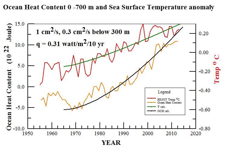
In these calculations, the aim was to find the heat input and thermal diffusivities necessary to account for the observed surface temperature increase (http://www.nodc.noaa.gov/OC5/3M_HEAT_CONTENT/ )Extended Reconstructed Sea Surface Temperature) and the increased ocean heat content (OHC 700) that have been reported by NOAA. Since surface temperatures had not been increasing in the early 1960s, but began to increase in the last half of that decade, I chose to start calculations with linearly increasing heating in 1965. I found that the ocean heat content to a depth of 700 meters was quite sensitive to the thermal diffusivity used. The best results that I have been able to obtain were for a thermal diffusivity of 1 cm2/s to 300 meter depth and surface heat input increasing at a rate of 0.31 watt/m2 per decade. These are shown on the graph below with calculated trends shown by the green and black lines. On a time scale of 50 years, most of the heat accumulates at relatively shallow depths. To better reflect a realistic thermal diffusivity for greater depths, I used a lower value of 0.3 cm2/s below 300 meter. That has little practical effect on a 50 year times scale, but would be necessary if one wanted to extend the calculations for several centuries while surface heating perturbations had time to penetrate to much greater depths.
http://i1244.photobucket.com/albums/gg580/stanrobertson/OHC700_zpsb9e34e91.jpg

Figure 1. Ocean heat content 0 – 700 meter and surface temperature trends according to NOAA. Blue and green lines show trends calculated for the parameters shown.
These calculations establish some parameters that do a good job of representing the thermal behavior of the upper oceans, however, if one looks closely at the data trends in the graph, it is apparent that both surface temperature and ocean heat content have considerably slowed their rates of increase in the last decade. This makes it unlikely that greenhouse gases are the cause of the rate of heating needed to explain the previous trends because their effects should have become enhanced rather than diminished. It might also be noted that a similar warming trend occurred in the first half of the previous century before anthropogenic greenhouse gases could have contributed significantly. Thus it is more likely that both warming periods had natural origins.
Obtaining simultaneous fits to the ocean heat content and sea surface temperature trends with only two free parameters, thermal diffusivity and surface heating rate, is quite confining. Acceptable, but noticeably worse, fits than shown above, were obtained with thermal diffusivities ranging from 0.8 to 1.2 cm2/s and heat inputs ranging from 0.29 to 0.33 watt/m2. Based on previous calculations for sea level data, I was initially inclined to think that larger thermal diffusivities would be necessary, but larger values let more heat penetrate to greater depths than the amounts of heat reported by Levitus et al. In addition, I was chagrined to learn that most of the variation of sea level that accompanies solar cycles is caused by evaporation rather than thermal expansion.
Solar Cycles:
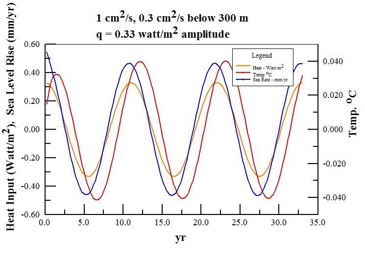
The process of choosing thermal diffusivity and surface heating rates to accord with observations provides a sound basis for calculating what to expect for the temperature variations during solar cycles. In this case we can use the thermal diffusivity of 1 cm2/s that is required of the ocean heat content results as an input parameter and choose the heat input that is required to produce temperature variations of 0.04 – 0.05 oC amplitude. Producing sea surface temperature variations with an amplitude of 0.04 oC requires a surface heat input of 0.33 watt/m2, as shown below:
http://i1244.photobucket.com/albums/gg580/stanrobertson/solarcycle10_zpsa3b8b0ee.jpg

Figure 2. Radiant flux, ocean temperature oscillations, and sea level variations for three solar cycles of eleven years each. The entering flux shown here is the value of q = 0.33 watt/m2 needed to drive the variations of surface temperature of 0.04 oC with ocean thermal diffusivity of 1.0 cm2/s to depth of 300 m. The amplitude of thermosteric rate of change of sea level was 0.47 mm/yr. Temperature lags the driving energy flux by 15 months. The thermal expansion coefficient of sea water used here was 2.4×10⁻⁴/ oC.
I believe that this settles the issue of what is required to produce sea surface temperature oscillations with an amplitude of 0.04 oC. The solar TSI variations that reach the earth’s surface are smaller than the 0.33 watt/m2 needed to account for sea surface temperature variations by a factor of 3.6 for this smallest estimate of sea surface temperature variability.
Although the estimated 0.33 watt/m2 that is required to explain the surface temperature variations is large compared to the amplitude of TSI variations that reach the surface, it is still only about two parts per thousand of the 160 watt/m2 of solar UV/VIS/NIR that reaches the earth surface. There are many possible ways in which the sun might modulate the surface energy flux to this extent. These include modulation of cloud cover and small spectral shifts in the energetic UV that might modulate ozone absorption or produce shifts of the effective sea surface albedo. It would seem to be a fairly direct radiative effect, rather than feedback, since it must vary in phase with the solar cycle.
In summary, my calculations based on energy conservation considerations imply that the sun modulates the ocean temperatures to a much greater extent than can be provided solely by its TSI variations. The great question that desperately needs an answer is how does it do it? It should be easily understood that solar effects would not necessarily be confined to cycles. More likely, the sun has been the driver of the large changes of temperatures of the Roman and Medieval warm period, the Little Ice Age, and the recent recovery from it without requiring large changes of its own irradiance. When we understand how the sun does this, we will have begun to understand the earthly climate.
###
Biographical note:
Stan Robertson, Ph.D, P.E, retired in 2004 after teaching physics at Southwestern Oklahoma State University for 14 years. In addition to teaching at three other universities over the years, he has maintained a consulting engineering practice for 30 years.
References:
Bryan, F., 1987: Parameter Sensitivity of Primitive Equation Ocean General Circulation Models. Journal of Physical Oceanography, 17, 970-985. (PDF available here http://journals.ametsoc.org/doi/abs/10.1175/1520-0485%281987%29017%3C0970%3APSOPEO%3E2.0.CO%3B2
Levitus, S. et al., 2012 World ocean heat content and thermosteric sea level change (0–2000 m), 1955–2010, Geophysical Research Letters, 39, L10603, doi:10.1029/2012GL051106, 2012 http://onlinelibrary.wiley.com/doi/10.1029/2012GL051106/abstract
Shaviv, Nir 2008, Using the oceans as a calorimeter to quantify the solar radiative forcing, Journal of Geophysical Research, 113, A11101 http://www.sciencebits.com/files/articles/CalorimeterFinal.pdf
Trenberth, K., Fasullo, J., Kiehl, J. 2009: Earth’s Global Energy Budget. Bull. Amer. Meteor. Soc., 90, 311–323. doi: http://dx.doi.org/10.1175/2008BAMS2634.1 www.cgd.ucar.edu/staff/trenbert/trenberth.papers/TFK_bams09.pdf , Fig. 1
Zhou, J. and Tung, K. ,2010 Solar Cycles in 150 Years of Global Sea Surface Temperature Data, Journal of Climate 23, 3234-3248 http://journals.ametsoc.org/doi/abs/10.1175/2010JCLI3232.1
The TSI may be very constant but variations in the energy output at particular frequencies may be important. For example changes in UV output are thought to affect ozone and cause differences in the complex photo chemistry. This in turn might modulate cloud seeding or aerosol behaviour. I don’t think that much is known about the chemistry of the atmosphere. I would imagine that a brew containing lots of subatomic particles, sulphuric acid, aerosols and lightening discharges, oxygen and ionised matter is capable of all sorts of interesting reactions.
I would imagine that aerosol particle size would have a major influence on light scattering and hence albedo. How much is known about the factors that influence the dispersion and flocculation of these particles?
I have a suspicion that solar influences are indirect but could be quite powerful.
Lief says, “….Otherwise the climate system would be a nifty energy producer: you put 10 units in and you get 36 out. I want one of those :-)”
I do that with potatoes in my garden. In fact I do better than that. I plant ten and on a good year can get 200.
Plankton may be small potatoes in the eyes of many, but I’ll bet it notices small changes in TSI. I won’t dare, (this early in the day,) risk any guesses about how much more energetic it becomes, or how the heck you could measure such energy.
Allan MacRae says: October 11, 2013 at 9:54 am
IF indeed the Sun is the primary controlling mechanism in the observed short-term (e.g. ~11 year Solar Cycles, ~80-90 year Gleissberg Cycles) warming and cooling periods that seem to correlate with minor solar variation according to many papers…
lsvalgaard says: October 11, 2013 at 10:03 am
This is precisely the sticking point. There are many claims. I probably know most of them put forward the last 350 years starting with Riccioli. I have yet to see one that is convincing. You could pick the one that is most convincing to you and we can discuss that one in detail.
Allan says:
Aye, there’s the rub.
I like Nir Shaviv’s work and that of Jan Veizer.
For the short term:
Shaviv, Nir 2008, Using the oceans as a calorimeter to quantify the solar radiative forcing, Journal of Geophysical Research, 113, A11101 http://www.sciencebits.com/files/articles/CalorimeterFinal.pdf
For the longer term
Nir J. Shaviv and Ján Veizer, Celestial driver of Phanerozoic climate? GSA Today July 2003 *
http://cfa.atmos.washington.edu/2003Q4/211/articles_optional/CelestialDriver.pdf
Best, Allan
* Turning and turning in the widening gyre
The falcon cannot hear the falconer;
Things fall apart; the centre cannot hold;
Mere anarchy is loosed upon the world…
– Yeats (1919)
lsvalgaard says:
“As there is almost no matter it matters not what the volume, temperature, and radiation are. If the volume were 1000 times larger and the temperature 10 times higher [both values much too high], the energy content would still be 100,000 times smaller than the lower atmosphere.”
The thermosphere is around 1/50,000 of the total atmospheric mass, and in parts the temperature reaches 2000°C at times. But then there is less troposphere in the polar regions.
Allan MacRae says:
October 11, 2013 at 10:41 am
For the longer term
Nir J. Shaviv and Ján Veizer, Celestial driver of Phanerozoic climate? GSA Today July 2003 *
Has already been debunked, see: Overholt et al. 2009 e.g. cited in http://www.leif.org/EOS/1303-7314-Cosmic-Rays-Climate-billion-yrs.pdf
For the short term:
Their Figure 4 is the actual data. The correlations are underwhelming, but if we apply a bit of good will as in Figure 5, we can see a SST swing of 0.1C which is what we would expect from TSI alone [this is undisputed], so if this is your strongest evidence I will agree with you that the observed variation of TSI gives rise to the observed variation of SST [all of 0.1C]. But I would not call that a major driver of climate.
Allan and Henry,
Could the earths response to TSI be more in terms of a delayed reaction by feedbacks than a direct heating by the average change to TSI? What I mean by a delayed reaction is that it takes a set amount of time for a feedback to react to a spike in TSI, so a large spike would give a lot more than average heating. Once the heating started, after a time, feedbacks (call it Eschenbach effect) mitigate the heating. An idea like this would not be impacted by “average TSI” because TSI is extremely spikey and the sun provides more than enough total energy to bake the earth if there were no negative feedback effects. What are your thoughts?
v/r,
David Riser
Ulric Lyons says:
October 11, 2013 at 11:10 am
The thermosphere is around 1/50,000 of the total atmospheric mass, and in parts the temperature reaches 2000°C at times.
assuming the most favorable case where the temperature is 2000C everywhere [which it is not] that temperature is 7 times that at sea level so the energy content is a 7/50,000 = 0.00014 part of the troposphere. Not much.
But then there is less troposphere in the polar regions.
And it is brrr cold there [I have lived there]
Thank you milon,
You are absolutely correct that educated people knew that Earth was round in Chaucer’s time.
A spherical Earth was reportedly proposed by Pythagoras in the 6th century BC.
Chaucer lived from ~1343 to 1400. And Chaucer was interested in astronomy, so he almost certainly knew Earth was round.
Copernicus published “De revolutionibus orbium coelestium” (On the Revolutions of the Celestial Spheres) in 1543, which re-arranged the planets and put the Sun in just the right spot.
But Newton did not publish his theory of gravitation until 1687, so until then everyone was really worried about falling off a round Earth into space. 🙂
This of course was no worse than sailing off the edge of a flat Earth, the chief concern of ancient mariners.
I mean, if you really watched your step on a round Earth (and parted your hair right down the middle), then you were probably OK.
But of course they were ALL wrong:
The world is really a flat plate supported on the back of a giant tortoise, on the back of another even bigger giant tortoise, etc. It’s tortoises all the way down.
This is the origin of the mathematical concept of infinity.
Best, Allan :-]
Meanwhile, back at the Turtles, all the way down:
http://en.wikipedia.org/wiki/Turtles_all_the_way_down
The most widely known version, which obviously is not the source (see below), appears in Stephen Hawking’s 1988 book A Brief History of Time, which starts:
A well-known scientist (some say it was Bertrand Russell) once gave a public lecture on astronomy. He described how the earth orbits around the sun and how the sun, in turn, orbits around the center of a vast collection of stars called our galaxy. At the end of the lecture, a little old lady at the back of the room got up and said: “What you have told us is rubbish. The world is really a flat plate supported on the back of a giant tortoise.” The scientist gave a superior smile before replying, “What is the tortoise standing on?” “You’re very clever, young man, very clever,” said the old lady. “But it’s tortoises all the way down!”
—Hawking, 1988[1]
In 1905, Oliver Corwin Sabin, Bishop of the Evangelical Christian Science Church, wrote:
The old original idea which was enunciated first in India, that the world was flat and stood on the back of an elephant, and the elephant did not have anything to stand on was the world’s thought for centuries. That story is not as good as the Richmond negro preachers who said the world was flat and stood on a turtle. They asked him what the turtle stood on and he said another turtle, and they asked what that turtle stood on and he said another turtle, and finally they got him in a hole and he said. “I tell you there are turtles all the way down.”
—Sabin, 1905[2]
Many 20th-century attributions point to William James as the source.[3][4] James referred to the fable of the elephant and tortoise several times, but told the infinite regress story with “rocks all the way down” in his 1882 essay, “Rationality, Activity and Faith”.[5] In the form of “rocks all the way down”, the story predates James to at least 1838.[6]
In 1854 the story in the current form appears, attributed by bible skeptic Joseph Barker to preacher Joseph Frederick Berg:
My opponent’s reasoning reminds me of the heathen, who, being asked on what the world stood, replied, “On a tortoise.” But on what does the tortoise stand? “On another tortoise.” With Mr. Barker, too, there are tortoises all the way down.
—Barker, 1854[7]
There is an allusion to the story in David Hume’s Dialogues Concerning Natural Religion (published in 1779):
How can we satisfy ourselves without going on in infinitum? And, after all, what satisfaction is there in that infinite progression? Let us remember the story of the Indian philosopher and his elephant. It was never more applicable than to the present subject. If the material world rests upon a similar ideal world, this ideal world must rest upon some other; and so on, without end. It were better, therefore, never to look beyond the present material world.
—Hume, 1779[8]
From Space Weather, Radio Active Sun: http://spaceweather.com/images2013/10oct13/Sr_Oct092013_2155ut2821_Ashcraft.mp3?PHPSESSID=rcodv060h40hjc02o0ud17nri4
Allan MacRae says:
October 11, 2013 at 11:24 am
Those mariners would have to be very ancient indeed, since the ancient Greeks knew that the world is a globe. They could see the shadow of the Earth upon the Moon during eclipses. More importantly when sailing, the mast of another ship appeared before its hull & the highest buildings in a port before the lower parts of the looming city.
Greek sailors also noted the variation in the observable altitude & change in the area of circumpolar stars apparent between their settlements around the Mediterranean & Black Seas, roughly Latitude 30 degrees to 47 degrees N. The difference grew more pronounced once Greeks went up the Nile under the Ptolemies. Eratosthenes managed to measure the Earth fairly accurately in Egypt, c. 240 BC.
lsvalgaard says: October 11, 2013 at 11:15 am
For the longer term
Nir J. Shaviv and Ján Veizer, Celestial driver of Phanerozoic climate? GSA Today July 2003 *
Has already been debunked, see: Overholt et al. 2009 e.g. cited in http://www.leif.org/EOS/1303-7314-Cosmic-Rays-Climate-billion-yrs.pdf
Allan says:
Debunked is a very big word that implies a very strong degree of scientific certainly.
Shaviv and Veizer GSA2003 was previously “debunked” in EOS circa 2003, but that “debunking”, as I recall, was purest guano.
I had a quick glance at Overholt et al and am not overly shaken, or stirred.
But thank you for the reference. I have had no time since 2008 to pursue this subject in the detail that it requires.
I am sincerely grateful for those like you who do.
Best personal regards, Allan
Illogical? Which other energy sources do you have in mind?
Allan MacRae says:
October 11, 2013 at 11:46 am
Bond, Cycle Bond…
Allan MacRae says:
October 11, 2013 at 11:46 am
Debunked is a very big word that implies a very strong degree of scientific certainly.
Actually not if the hypothesis being debunked is itself on shaky ground, i.e. has little certainty to begin with.
milodonharlani says:
October 11, 2013 at 11:50 am
Bond, Cycle Bond…
There are no Bond cycles. There may be some variability of 1000-2000 yr time scale but they are not cyclic.
Thank you, Dr. Svalgaard (and Pamela and others above), after reading the above I believe I understand what the facts are. Here is what a non-scientist concluded from your fine teaching. I hope this encourages you, Dr. Svalgaard, for, hopefully, it shows that your teaching is good enough to help even a non-scientist learn. (Note: if I’m actually all mixed up, just ignore me — it isn’t your fault and I’m far too ignorant of the basics for you to waste any time correcting.)
The current state of our knowledge includes the following (list NOT exhaustive of what I learned above, just limited for sake of time):
1. While TSI can vary the surface temperature of the ocean, overall, it maintains sea surface (and, later, land surface) temperature; further, it cannot (by a magnitude of 3) heat the sub-surface depths to a measurable degree.
2. All Sun forces other than TSI are negligible v. a v. heating Earth.
3. “Cyclic” is an inaccurate term, here, for the peaks and valleys are not uniform.
4. The Earth’s tilting causes seasonal temperature variation; Sun’s input remains essentially constant.
5. While the Sun, like a human heart (not a perfect parallel, I realize), provides the basic energy for warmth, it does not cause any significant variation in the energy in Earth’s climate system.
The Sun is the homeostatic energy supplied by the heart that enables a violinist to simply live. It is the muscles in the arm and fingers that cause the variations in pitch, tempo, and dynamics that create beautiful (or ugly) music. Should the violinist faint and fall to the ground, the music would stop. That this would happen does not mean that the heart itself creates the variations that make the music a delight (or an annoyance). If the violinist tips the bottle a few too many times, altering his or her equilibrium, just before performing, the music will be affected, but the heart does not change.
In sum: The truism that, but for the heart’s beating, there would be no music
does NOT lead to the conclusion that music is caused by the heart.
lsvalgaard says:
October 11, 2013 at 12:01 pm
Some of your colleagues once dared to disagree. Maybe not solar-driven cycles at that frequency, but perhaps oceanic, although admittedly this wavelet analysis study (citing many of the usual “climate science” suspects) is from way back in 2007:
http://hal.archives-ouvertes.fr/hal-00330766/
The origin of the 1500-year climate cycles in Holocene North-Atlantic records
M. Debret 1, V. Bout-Roumazeilles 2, F. Grousset 3, Marc Desmet 4, J. F. Mcmanus 5, N. Massei 6, D. Sebag 6, J.-R. Petit 1, Y. Copard 6, A. Trentesaux 2
(01/10/2007)
Since the first suggestion of 1500-year cycles in the advance and retreat of glaciers (Denton and Karlen, 1973), many studies have uncovered evidence of repeated climate oscillations of 2500, 1500, and 1000 years. During last glacial period, natural climate cycles of 1500 years appear to be persistent (Bond and Lotti, 1995) and remarkably regular (Mayewski et al., 1997; Rahmstorf, 2003), yet the origin of this pacing during the Holocene remains a mystery (Rahmstorf, 2003), making it one of the outstanding puzzles of climate variability. Solar variability is often considered likely to be responsible for such cyclicities, but the evidence for solar forcing is difficult to evaluate within available data series due to the shortcomings of conventional time-series analyses. However, the wavelets analysis method is appropriate when considering non-stationary variability. Here we show by the use of wavelets analysis that it is possible to distinguish solar forcing of 1000- and 2500- year oscillations from oceanic forcing of 1500-year cycles. Using this method, the relative contribution of solar-related and ocean-related climate influences can be distinguished throughout the 10 000 yr Holocene intervals since the last ice age. These results reveal that the 1500-year climate cycles are linked with the oceanic circulation and not with variations in solar output as previously argued (Bond et al., 2001). In this light, previously studied marine sediment (Bianchi and McCave, 1999; Chapman and Shackleton, 2000; Giraudeau et al., 2000), ice core (O’Brien et al., 1995; Vonmoos et al., 2006) and dust records (Jackson et al., 2005) can be seen to contain the evidence of combined forcing mechanisms, whose relative influences varied during the course of the Holocene. Circum-Atlantic climate records cannot be explained exclusively by solar forcing, but require changes in ocean circulation, as suggested previously (Broecker et al., 2001; McManus et al., 1999).
milodonharlani says:
October 11, 2013 at 12:16 pm
Some of your colleagues once dared to disagree. Maybe not solar-driven cycles at that frequency, but perhaps oceanic, although admittedly this wavelet analysis study (citing many of the usual “climate science” suspects) is from way back in 2007
It is a good idea to keep up with the literature:
http://www.leif.org/EOS/Obrochta2012.pdf
Hint: I would not make my statement without having something to back it up with.
Prove your comment isn’t fatuous, Steve.
For the short term:
Shaviv, Nir 2008, Using the oceans as a calorimeter to quantify the solar radiative forcing, Journal of Geophysical Research, 113, A11101 http://www.sciencebits.com/files/articles/CalorimeterFinal.pdf
lsvalgaard says: October 11, 2013 at 11:15 am
Their Figure 4 is the actual data. The correlations are underwhelming,
Allan says:
The correlations are less than perfect, but are not too bad, imo.
If I recall correctly, you made the same comment about the less than perfect correlations (dCO2/dt vs temperature T and atmospheric CO2 LAGS temperature) in my 2008 icecap.us paper.
My 2008 hypo has stood up quite well, although it made warmists very uncomfortable, and was dismissed as a “feedback effect” until Salby revived the concept in circa 2011.
You were in good company re 2008 – Willis et al objected strongly to “Spurious Correlation and Data Smoothing” on ClimateAudit.org but it appears all of you were wrong. But none of this is bad – it is all a necessary part of the process.
The only part that amused me was when Pieter Tans published the same conclusion, all opposition suddenly vanished, and Tans did not even supply his data – just some graphs. So much for a level playing field.
But everyone can be wrong Leif, and nobody likes it when they are. I know. I was wrong once as a child, and vowed to never do it again. :-}
Leif again:
… but if we apply a bit of good will as in Figure 5, we can see a SST swing of 0.1C which is what we would expect from TSI alone [this is undisputed], so if this is your strongest evidence I will agree with you that the observed variation of TSI gives rise to the observed variation of SST [all of 0.1C]. But I would not call that a major driver of climate.
Allan says:
Is your above statement inconsistent with this quote from the Abstract?
We find that the total radiative forcing associated with solar cycles variations is about 5 to 7 times larger than just those associated with the TSI variations, thus implying the necessary existence of an amplification mechanism, though without pointing to which one.
Best, Allan
lsvalgaard says:
October 11, 2013 at 12:21 pm
I didn’t suppose that you lacked support for your position. Sorry if you took my comments in that way. I do try to keep up on the literature, but admit to not having read the 2012 paper.
The paper that I cited & your 2012 study aren’t necessarily contradictory, IMO. Both find or accept the 1000-2000 year solar signal which you granted might exist. Your citation doesn’t conclusively falsify the existence of the oceanic cycle observed in the 2007 paper. It shows that the 1500-year signal at one DSDP site might be spurious. IMO it’s premature to draw from this finding, perhaps debatable, the conclusion that Bond Cycles don’t exist at all. If they do, they’re likely to result from the combination of solar & oceanic effects, as appears to be the case with their stronger big brothers during glacial times, the well-established D-O cycles.
Allan MacRae says:
October 11, 2013 at 12:36 pm
The correlations are less than perfect, but are not too bad, imo.
If we accept them then they show that the SST variation is simply accounted for by TSI variations [of the expected 0.1C]
If I recall correctly, you made the same comment about the less than perfect correlations
A crummy correlation is still crummy, it could be real, but that one crummy correlation turned out to hold does not mean that other crummy correlations also hold.
Is your above statement inconsistent with this quote from the Abstract?
I would say that the abstract is at variance with my statement. The 0.1C is what I always expected and it seems that Shaviv has also found it.
milodonharlani says:
October 11, 2013 at 12:38 pm
If they do, they’re likely to result from the combination of solar & oceanic effects, as appears to be the case with their stronger big brothers during glacial times, the well-established D-O cycles.
The D-O cycles have a natural explanation as terrestrial effects. No need to invoke the Sun: http://www.leif.org/EOS/palo20005-D-O-Explanation.pdf
milodonharlani says: October 11, 2013 at 11:42 am
Those mariners would have to be very ancient indeed, since the ancient Greeks knew that the world is a globe. They could see the shadow of the Earth upon the Moon during eclipses.
Allan says:
Do you really think they were so advanced then during a lunar eclipse?
I understand that around the world they beat drums, threw sticks and shouted loudly to scare off the great animal that had eaten the moon.
Some also sacrificed a virgin, if they could find one.
in climatology …you don’t take the temperature of a system but a location…( and some even use the second principle of thermodynamics with that..)
to change the temperature of a location you don’t have to heat but move..
the temp signal has both circulation and heat signification.
So it may not be an amplification but a change in circulation pattern according with the sun.
And Hockey Schtick has an excellent point above on the measurable global brightness which must simultaneously be wrapped into any causes. Bound to me multi-pronged.