Climate Dialogue about the (missing) hot spot
by Marcel Crok
Over at the Climate Dialogue website we start with what could become a very interesting discussion about the so-called tropical hot spot. Climate models show amplified warming high in the tropical troposphere due to greenhouse forcing. However data from satellites and weather balloons don’t show much amplification. What to make of this? Have the models been ‘falsified’ as critics say or are the errors in the data so large that we cannot conclude much at all? And does it matter if there is no hot spot?
The (missing) tropical hot spot is one of the long-standing controversies in climate science. In 2008 two papers were published, one by a few scientists critical of the IPCC view (Douglass, Christy, Pearson and Singer) and one by Ben Santer and sixteen other scientists. We have participants from both papers. John Christy is the ‘representative’ from the first paper and Steven Sherwood and Carl Mears are ‘representatives’ of the second paper.
Below I repost the introduction that we – the editors of Climate Dialogue – prepared as the basis for the discussion.
The (missing) hot spot in the tropics
Based on theoretical considerations and simulations with General Circulation Models (GCMs), it is expected that any warming at the surface will be amplified in the upper troposphere. The reason for this is quite simple.
More warming at the surface means more evaporation and more convection. Higher in the troposphere the (extra) water vapour condenses and heat is released. Calculations with GCMs show that the lower troposphere warms about 1.2 times faster than the surface. For the tropics, where most of the moist is, the amplification is larger, about 1.4.
This change in thermal structure of the troposphere is known as the lapse rate feedback. It is a negative feedback, i.e. attenuating the surface temperature response due to whatever cause, since the additional condensation heat in the upper air results in more radiative heat loss.
IPCC published the following figure in its latest report (AR4) in 2007:

Source: http://www.ipcc.ch/publications_and_data/ar4/wg1/en/figure-9-1.html (based on Santer 2003)
The figure shows the response of the atmosphere to different forcings in a GCM. As one can see, over the past century, the greenhouse forcing was expected to dominate all other forcings. The expected warming is highest in the tropical troposphere, dubbed the tropical hot spot.
The discrepancy between the strength of the hot spot in the models and the observations has been a controversial topic in climate science for almost 25 years. The controversy [i] goes all the way back to the first paper of Roy Spencer and John Christy [ii] about their UAH tropospheric temperature dataset in the early nineties. At the time their data didn’t show warming of the troposphere. Later a second group (Carl Mears and Frank Wentz of RSS) joined in, using the same satellite data to convert them into a time series of the tropospheric temperature. Several corrections, e.g. for the orbital changes of the satellite, were made in the course of years with a warming trend as a result. However the controversy remains because the tropical troposphere is still showing a smaller amplification of the surface warming which is contrary to expectations.
Positions
Some researchers claim that observations don’t show the tropical hot spot and that the differences between models and observations are statistically significant [iii]. On top of that they note that the warming trend itself is much larger in the models than in the observations (see figure 2 below and also ref. [iv]). Other researchers conclude that the differences between the trends of tropical tropospheric temperatures in observations and models are statistically not inconsistent with each other [v]. They note that some radiosonde and satellite datasets (RSS) do show warming trends comparable with the models (see figure 3 below).
The debate is complex because there are several observational datasets, based on satellite (UAH and RSS) but also on radiosonde measurements (weather balloons). Which of the dataset is “best” and how does one determine the uncertainty in both datasets and model simulations?
The controversy flared up in 2007/2008 with the publications of two papers [vi][vii] of the opposing groups. Key graphs in both papers are the best way to give an impression of the debate. First Douglass et al. came up with the following graph showing the disagreement between models and observations:

Figure 2. Temperature trends for the satellite era. Plot of temperature trend (°C/decade) against pressure (altitude). The HadCRUT2v surface trend value is a large blue circle. The GHCN and the GISS surface values are the open rectangle and diamond. The four radiosonde results (IGRA, RATPAC, HadAT2, and RAOBCORE) are shown in blue, light blue, green, and purple respectively. The two UAH MSU data points are shown as gold-filled diamonds and the RSS MSU data points as gold-filled squares. The 22-model ensemble average is a solid red line. The 22-model average ±2σSE are shown as lighter red lines. MSU values of T2LT and T2 are shown in the panel to the right. UAH values are yellow-filled diamonds, RSS are yellow-filled squares, and UMD is a yellow-filled circle. Synthetic model values are shown as white-filled circles, with 2σSE uncertainty limits as error bars. Source: Douglass et al. 2008
Santer et al. criticized Douglass et al. for underestimating the uncertainties in both model output and observations and also for not showing all radiosonde datasets. They came up with the following graph:

Figure 3. Vertical profiles of trends in atmospheric temperature (panel A) and in actual and synthetic MSU temperatures (panel B). All trends were calculated using monthly-mean anomaly data, spatially averaged over 20 °N–20 °S. Results in panel A are from seven radiosonde datasets (RATPAC-A, RICH, HadAT2, IUK, and three versions of RAOBCORE; see Section 2.1.2) and 19 different climate models. The grey-shaded envelope is the 2σ standard deviation of the ensemble-mean trends at discrete pressure levels. The yellow envelope represents 2σSE, DCPS07’s estimate of uncertainty in the mean trend. The analysis period is January 1979 through December 1999, the period of maximum overlap between the observations and most of the model 20CEN simulations. Note that DCPS07 used the same analysis period for model data, but calculated all observed trends over 1979–2004. Source: Santer (2008)
The grey-shaded envelope is the 2σ standard deviation of the ensemble-mean trends of Santer et al. while the yellow band is the estimated uncertainty of Douglass et al. Some radiosonde series in the Santer graph (like the Raobcore 1.4 dataset) show even more warming higher up in the troposphere than the model mean.
Updates
Not surprisingly the debate didn’t end there. In 2010 McKitrick et al. [viii] updated the results of Santer (2008), who limited the comparison between models and observations to the period 1979-1999, to 2009. They concluded that over the interval 1979–2009, model projected temperature trends are two to four times larger than observed trends in both the lower troposphere and the mid troposphere and the differences are statistically significant at the 99% level.
Christy (2010)[ix] analysed the different datasets used and concluded that some should be discarded in the tropics:

Figure 4. Temperature trends in the lower tropical troposphere for different datasets and for slightly differing periods (79-05 = 1979-2005). UAH and RSS are the estimates based on satellite measurements. HadAt, Ratpac, RC1.4 and Rich are based on radiosonde measurements. C10 and AS08 [x] are based on thermal wind data. The other three datasets give trends at the surface (ERSST being for the oceans only while the other two combine land and ocean data). Source: Christy (2010)
Christy (2010) concluded that part of the tropical warming in the RSS series is spurious. They also discarded the indirect estimates that are based on thermal wind. Not surprisingly Mears (2012) disagreed with Christy’s conclusion about the RSS trend being spurious writing that “trying to determine which MSU [satellite] data set is “better” based on short-time period comparisons with radiosonde data sets alone cannot lead to robust conclusions”.[xi]
Scaling ratio
Christy (2010) also introduced what they called the “scaling ratio”, the ratio of tropospheric to surface trends and concluded that these scaling ratios clearly differ between models and observations. Models show a ratio of 1.4 in the tropics (meaning troposphere warming 1.4 times faster than the surface), while the observations have a ratio of 0.8 (meaning surface warming faster than the troposphere). Christy speculated that an alternate reason for the discrepancy could be that the reported trends in temperatures at the surface are spatially inaccurate and are actually less positive. A similar hypothesis was tested by Klotzbach (2009).[xii]
In an extensive review article about the controversy published in early 2011 Thorne et al. ended with the conclusion that “there is no reasonable evidence of a fundamental disagreement between tropospheric temperature trends from models and observations when uncertainties in both are treated comprehensively”. However in the same year Fu et al.[xiii] concluded that while “satellite MSU/AMSU observations generally support GCM results with tropical deep‐layer tropospheric warming faster than surface, it is evident that the AR4 GCMs exaggerate the increase in static stability between tropical middle and upper troposphere during the last three decades”. More papers then started to acknowledge that the consistency of tropical tropospheric temperature trends with climate model expectations remains contentious.[xiv][xv][xvi][xvii]
Climate Dialogue
We will focus the discussion on the tropics as the hot spot is most pronounced there in the models. Core questions are of course whether we can detect/have detected a hot spot in the observations and if not what are the implications for the reliability of GCMs and our understanding of the climate?
Specific questions
1) Do the discussants agree that amplified warming in the tropical troposphere is expected?
2) Can the hot spot in the tropics be regarded as a fingerprint of greenhouse warming?
3) Is there a significant difference between modelled and observed amplification of surface trends in the tropical troposphere (as diagnosed by e.g. the scaling ratio)?
4) What could explain the relatively large difference in tropical trends between the UAH and the RSS dataset?
5) What explanation(s) do you favour regarding the apparent discrepancy surrounding the tropical hot spot? A few options come to mind: a) satellite data show too little warming b) surface data show too much warming c) within the uncertainties of both there is no significant discrepancy d) the theory (of moist convection leading to more tropospheric than surface warming) overestimates the magnitude of the hotspot
6) What consequences, if any, would your explanation have for our estimate of the lapse rate feedback, water vapour feedback and climate sensitivity?
[i] Thorne, P. W. et al., 2011, Tropospheric temperature trends: History ofan ongoing controversy. WIRES: Climate Change, 2: 66-88
[ii]Spencer RW, Christy JR. Precise monitoring of global temperature trends from satellites. Science 1990, 247:1558–1562.
[iii] Christy, J. R., B. M. Herman, R. Pielke Sr., P. Klotzbach, R. T. McNider, J. J. Hnilo, R. W. Spencer, T. Chase, and D. H. Douglass (2010), What do observational datasets say about modeled tropospheric temperature trends since 1979?, Remote Sens., 2, 2148–2169, doi:10.3390/rs2092148.
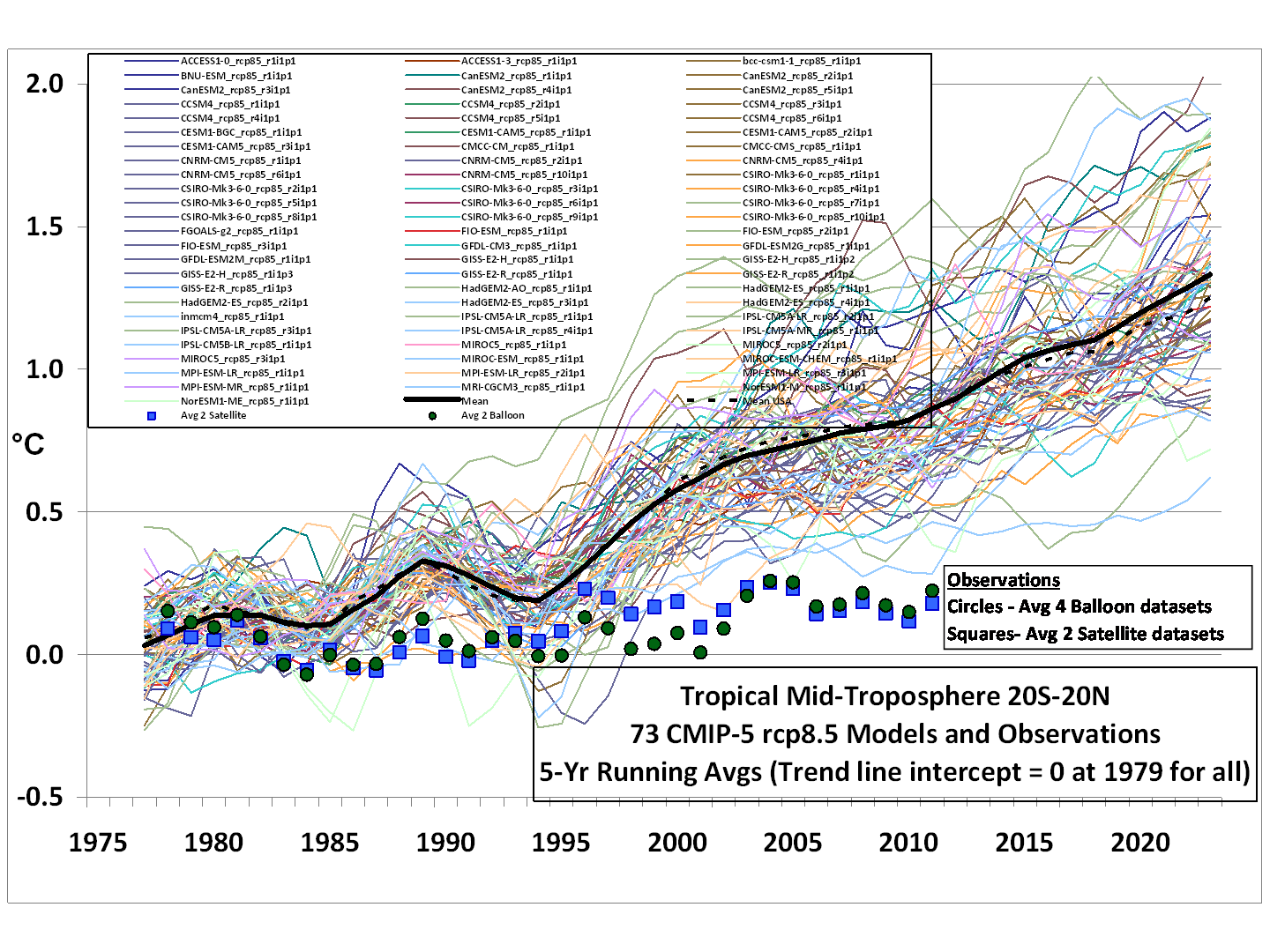
[iv]http://www.drroyspencer.com/wp-content/uploads/CMIP5-73-models-vs-obs-20N-20S-MT-5-yr-means1.png
[v]Thorne, P.W. Atmospheric science: The answer is blowing in the wind. Nature Geosci. 2008, doi:10.1038/ngeo209
[vi] Douglass DH, Christy JR, Pearson BD, Singer SF. A comparison of tropical temperature trends with model predictions. Int J Climatol 2008, 27:1693–1701
[vii] Santer, B.D.; Thorne, P.W.; Haimberger, L.; Taylor, K.E.; Wigley, T.M.L.; Lanzante, J.R.; Solomon, S.; Free, M.; Gleckler, P.J.; Jones, P.D.; Karl, T.R.; Klein, S.A.; Mears, C.; Nychka, D.; Schmidt, G.A.; Sherwood, S.C.; Wentz, F.J. Consistency of modelled and observed temperature trends in the tropical troposphere. Int. J. Climatol. 2008, doi:1002/joc.1756
[viii] McKitrick, R. R., S. McIntyre and C. Herman (2010) “Panel and Multivariate Methods for Tests of Trend Equivalence in Climate Data Sets.” Atmospheric Science Letters, 11(4) pp. 270-277, October/December 2010 DOI: 10.1002/asl.290
[ix] Christy, J. R., B. M. Herman, R. Pielke Sr., P. Klotzbach, R. T. McNider, J. J. Hnilo, R. W. Spencer, T. Chase, and D. H. Douglass (2010), What do observational datasets say about modeled tropospheric temperature trends since 1979?, Remote Sens., 2, 2148–2169, doi:10.3390/rs2092148
[x] Allen RJ, Sherwood SC. Warming maximum in the tropical upper troposphere deduced from thermal winds. Nat Geosci 008, 1:399–403
[xi] Mears, C. A., F. J. Wentz, and P. W. Thorne (2012), Assessing the value of Microwave Sounding Unit–radiosonde comparisons in ascertaining errors in climate data records of tropospheric temperatures, J. Geophys. Res., 117, D19103, doi:10.1029/2012JD017710
[xii] Klotzbach PJ, Pielke RA Sr., Pielke RA Jr., Christy JR, McNider RT. An alternative explanation for differential temperature trends at the surface and in the lower troposphere. J Geophys Res 2009, 114:D21102. DOI:10.1029/2009JD011841
[xiii] Fu, Q., S. Manabe, and C. M. Johanson (2011), On the warming in the tropical upper troposphere: Models versus observations, Geophys. Res. Lett., 38, L15704, doi:10.1029/2011GL048101
[xiv] Seidel, D. J., M. Free, and J. S. Wang (2012), Reexamining the warming in the tropical upper troposphere: Models versus radiosonde observations, Geophys. Res. Lett., 39, L22701, doi:10.1029/2012GL053850
[xv] Po-Chedley, S., and Q. Fu (2012), Discrepancies in tropical upper tropospheric warming between atmospheric circulation models and satellites, Environ. Res. Lett
[xvi] Benjamin D. Santer, Jeffrey F. Painter, Carl A. Mears, Charles Doutriaux, Peter Caldwell, Julie M. Arblaster, Philip J. Cameron-Smith, Nathan P. Gillett, Peter J. Gleckler, John Lanzante, Judith Perlwitz, Susan Solomon, Peter A. Stott, Karl E. Taylor, Laurent Terray, Peter W. Thorne, Michael F. Wehner, Frank J. Wentz, Tom M. L. Wigley, Laura J. Wilcox, and Cheng-Zhi Zou, Identifying human influences on atmospheric temperature, PNAS 2013 110 (1) 26-33; published ahead of print November 29, 2012, doi:10.1073/pnas.1210514109
[xvii] Thorne, P. W., et al. (2011), A quantification of uncertainties in historical tropical tropospheric temperature trends from radiosondes, J. Geophys. Res., 116, D12116, doi:10.1029/2010JD015487
Discover more from Watts Up With That?
Subscribe to get the latest posts sent to your email.
A lot of topics address here at WUWT seem appropriate. Miskolczi (sp?) was the one of the first to claim a constant GHE. That is, as CO2 increases the amount of H2O decreases accordingly. Joe B’s description of a reduction in RH would support this theory. I’ve also heard people mentioned an increase in the partial pressure of CO2 must be causing a reduction in other gases. This just might be H2O given its variability.
It all seems to fit together and support a very stable equilibrium situation. Of course, for a planet to survive a billion of years of life sustaining climate, one might just think it was pretty stable.
Bob is right of course.
This is simply because the climate scientists refuse to acknowledge the natural cycles in climate. It just so happens that during most of the satellite era PDO was positive (or like Bob will probably prefer, ENSO was high) and then tropical Pacific do not warm much. Now that the cycle has turned ironically we will probably see the hot spot in a decade or two, after a long pause in global warming but warming of the tropics and cooling around 30-40 lat. Tropical and mid latitude Pacific simply do not warm at the same time.
My modified version of Bobs graph, http://virakkraft.com/PDO-fingerprint-Pacific.png
More people are starting to get it 🙂
Or understood all along but are now gaining the confidence to say it.
Mother Nature’s tower heat sinks (aka tropical thunderstorms) pipeline heat into space. That also explains the missing H20 positive feedback. The negative feedback due to this pipelining overwhelms any positive components.
“””””…..davidmhoffer says:
July 16, 2013 at 10:15 pm
2) Can the hot spot in the tropics be regarded as a fingerprint of greenhouse warming?
No, nor can the absence of one be construed as lack thereof.
We know a great deal about how CO2 interacts with LW in a lab setting. That allows us to extrapolate theories as to how it MIGHT change the atmospheric system as a whole. …..”””””
David, I don’t have much quarrel with the claimed LWIR absorption/emission properties of the CO2 molecule. I’m not a physical chemist, but I believe that is a robust discipline, that is theoretically well understood.
But the atmospheric phenomenon is how the CO2 molecule as a dilute component of a complex atmosphere interacts with the ambient LWIR radiation that is primarily sourced from the earth surface (solid/liquid).
So I am totally deaf to “lab experiments” where CO2 gas mixtures are subjected to radiation sources that are ten times the real earth ambient source Temperature, and therefore 10,000 times as bright as the earth surface, and emitting a completely different spectrum at one tenth of the real LWIR wavelengths, which have completely different interactions with the CO2.
Has anyone actually done any “real” laboratory experiments with CO2 mixtures, using a real 288 Kelvin thermal radiation source that is putting out a 10.1 micron peak wavelength emission spectrum at about 390 W/m^2.
There would need to be some serious cooling of the apparatus to eliminate ambient 288 K emissions from the whole damn laboratory.
How can the earth be radiating a crude BB type spectrum corresponding to the surface Temperature when Trenberth claims that only 40 W/m^2 escapes to space in the atmospheric window, and folks insist that the main body of the atmosphere (gases) does not emit thermal radiation. Well of course I don’t believe that last assertion. Gases do emit thermal radiation continuum spectra; it just isn’t black body radiation. Well nothing emits black body radiation; just a sometimes fairly close but limited spectra approximation.
george e smith;
Has anyone actually done any “real” laboratory experiments with CO2 mixtures, using a real 288 Kelvin thermal radiation source that is putting out a 10.1 micron peak wavelength emission spectrum at about 390 W/m^2.
>>>>>>>>>>>>>.
Yes.
http://www.john-daly.com/artifact.htm
However I don’t consider this directly relevant to what happens in the atmosphere as a whole. Hug’s apparatus was 10 cm in length, the atmospheric air column is many kilometers, not the same thing at all. Plus no convection, condensation, or evaporation etc etc etc in Hug’s experiment either. In other words, CO2 in isolation at two different concentrations to see what happens.
Was the hypothis of a hotspot in Earth’s atmosphere caused because of the red spot on Venus?
CC Squid says:
July 17, 2013 at 12:09 pm
Was the hypothis of a hotspot in Earth’s atmosphere caused because of the red spot on Venus?
>>>>>>>>>
The reasoning for the existence is contained in the article.
The lapse rate feedback is only a negative feedback (in the general circulation model) if the long wave radiation that is released when the water vapour condenses is emitted to space rather than trapped by increased water vapour. Higher modelled temperature in the troposphere enables the general circulation model to assume there is more water vapour in the troposphere which amplifies the CO2 forcing by increasing the amount of water vapor in troposphere.
If the objective was to develop a general circulation model that matches reality rather than to push an agenda likely one of model fixes would be modify to GCMs (modeling of planetary cloud cover) to match Lindzen and Choi finding that planetary cloud cover in the tropics increases or decreases to resist forcing changes by reflecting more or less radiation off to space.
It appears other general circulation model fixes are required as there is a fairly long list of unexplained anomalies. There is currently no logical explanation as to 1) why there has been a 16 year period where there is a plateau of no warming and 2) why the majority of the warming in the last 70 years has been in high latitude regions in the Northern hemisphere, 4) why there is no tropical tropospheric hot spot 5) why there is cyclic warming in the paleo record where the same regions that warmed in the last 70 years, and 6) why there are solar magnetic changes that correlate with past cyclic warming and cooling (TSI changes to the sun do not explain the cyclic warming and cooling).
Comment:
1. A plateau where there is no warming is more difficult to explain than a wiggly gradual increase in temperature where the rate of increase is less than predicted. As the CO2 forcing mechanism cannot be turned on and off there needs to be a smart mechanism that hides the CO2 forcing. The aerosol hypothesis appears to fail as the aerosols are emitted in the Northern hemisphere where there is the most amount of warming. The aerosol hypothesis requires there to be less warming in the Northern hemisphere rather more warming.
2. The ex-tropic region of the Northern hemisphere has warmed twice as much as the planet as a whole and four times as much as the tropics. Furthermore the Greenland Ice Sheet has warmed the most of any region on the planet.
3. The same pattern of warming has occurred before. A mechanism than modulates planetary cloud cover could explain regional warming. Curiously the regions where the warming occurred are also the regions that are most strongly affected by solar mechanisms that modulate planetary cloud cover.
It seems the GCM were specifically written to produce amplification, using the modeling assumptions.
http://typhoon.atmos.colostate.edu/Includes/Documents/Publications/gray2012.pdf
The Physical Flaws of the Global Warming Theory and Deep Ocean Circulation Changes as the Primary Climate Driver
The water vapor, cloud, and condensation-evaporation assumptions within the conventional AGW theory and the (GCM) simulations are incorrectly designed to block too much infrared (IR) radiation to space. They also do not reflect-scatter enough short wave (albedo) energy to space. These two misrepresentations result in a large artificial warming that is not realistic. A realistic treatment of the hydrologic cycle would show that the influence of a doubling of CO2 should lead to a global surface warming of only about 0.3°C – not the 3°C warming as indicated by the climate simulations…. ….The NAS or Charney Report of 1979. The basic error of the global GCMs has been the model builder’s general belief in the National Academy of Science (NAS) 1979 study – often referred to as The Charney Report – which hypothesized that a doubling of atmospheric CO2 would bring about a general warming of the globe’s mean temperature between 1.5 – 4.5°C (or an average of ~ 3.0°C) (Figure 5). This was based on the report’s assumption that the relative humidity (RH) of the atmosphere would remain quasi-constant as the globe’s temperature increased from CO2‘s influence to block IR energy loss to space. The Clausius-Clapeyron equation specifies that as the temperature of the air rises the ability of the air to hold more water vapor rises exponentially. If relative humidity (RH) of the air were to remain constant as atmospheric temperature rose then the water vapor (q) amount in the atmosphere would accordingly rise. The water vapor content of the atmosphere rises by about 50 percent if atmospheric temperatures were to increase by 5C and relative humidity remained constant. Rising water vapor content, particularly in the upper troposphere greatly reduce the amount of outgoing longwave radiation (OLR) which can escape to space.
http://www-eaps.mit.edu/faculty/lindzen/236-Lindzen-Choi-2011.pdf
On the Observational Determination of Climate Sensitivity and Its Implications
Richard S. Lindzen1 and Yong-Sang Choi2
Idso’s classic paper is interesting as Idso uses real world data to estimate the planet’s response to a change in feedback. The results of Idso’s analysis supports the assertion that the warming due to a doubling of atmospheric CO2 would be roughly 0.3C.
Idso Skeptics View of Global Warming
http://www.mitosyfraudes.org/idso98.pdf
“””””…..William Astley says:
July 17, 2013 at 1:39 pm
The lapse rate feedback is only a negative feedback (in the general circulation model) if the long wave radiation that is released when the water vapour condenses is emitted to space rather than trapped by increased water vapour. …..”””””
So far as I am aware, the process of condensation of water vapor, to form liquid water, is a purely thermal process; not a radiative process.
So there is no release of LWIR radiation due to condensation. Nothing heats up (increases in Temperature) as a consequence of condensation of water vapor; it won’t condense unless it is cooled down.
“””””…..davidmhoffer says:
July 17, 2013 at 11:15 am
george e smith;
Has anyone actually done any “real” laboratory experiments with CO2 mixtures, using a real 288 Kelvin thermal radiation source that is putting out a 10.1 micron peak wavelength emission spectrum at about 390 W/m^2.
>>>>>>>>>>>>>.
Yes.
http://www.john-daly.com/artifact.htm……..”””””””””
Well I read that paper, and it distinctly says they used a 1,000 to 1,200 deg C source for their infrared radiation. That is not even approximately comparable to a 288 Kelvin source.
A chilled bottle of water, would be a much closer to reality source of the appropriate radiation.
Their source is about 517 times brighter than the real world source.
And I do believe I said in my post, that any lab result would not replicate what happens in the real atmosphere.
george;
Well I read that paper, and it distinctly says they used a 1,000 to 1,200 deg C source for their infrared radiation.
>>>>>>>>>>>>>>
which they filtered to obtain the desired range.
I think the reason there is no hotspot in the troposphere is because a large part of the convective mechanism is coupled with thunderstorms (a la Willis Eschenbach) in the tropics. BTW, this “thermostat” is what puts a 31C upper limit on sea surface temperature. The troposphere is 6 to 10km above the surface and the thunderstorm chimneys rush the moist hot air rapidly up as high as 15+km. Where, in the thin air of this altitude, it radiates readily to space. These rapidly rising columns by-pass the troposphere. Certainly in this environment there is no chance for significant downwelling LWIR, either. Also,do models account adequately for the non-temperature enthalpy of these phenomena – kinetic energy of winds, falling rain and ice, electricity generated…
To build on what davidmhoffer pointed out: the real question is why do the AGW promoters decline to review their models and assumptions in the face of significant data- slr, OA, troposphere, weather patterns, etc. that do not support their predictions?
“””””…..davidmhoffer says:
July 17, 2013 at 3:15 pm
george;
Well I read that paper, and it distinctly says they used a 1,000 to 1,200 deg C source for their infrared radiation.
>>>>>>>>>>>>>>
which they filtered to obtain the desired range…….””””””
David, I’m highly suspicious of filters. Many types of filters which do attenuate a specific input wavelength, have a nasty habit of simply passing the energy on at a different wavelength. (Beer’s law simply doesn’t hold for the ENERGY TRANSMISSION).
But I’m quite happy to accept that you believe it’s a credible methodology.
Thanx
In reply to:
george e. smith says:
July 17, 2013 at 2:41 pm
“””””…..William Astley says:
July 17, 2013 at 1:39 pm
The lapse rate feedback is only a negative feedback (in the general circulation model) if the long wave radiation that is released when the water vapour condenses is emitted to space rather than trapped by increased water vapour. …..”””””
So far as I am aware, the process of condensation of water vapor, to form liquid water, is a purely thermal process; not a radiative process.
William;
Yes. I agree with your comment. Water evapourating and then condensing moves energy from the ocean to higher in the atmosphere, there is no radiation involved with condensing. My comment above was incorrect.
I will try again.
It appears the key issue (reality/observations Vs GCM) is how much water vapour condensates.
The increased atmospheric CO2 will cause an increase in ocean temperature which will cause an increase in water vapour.
The key question is does an increase in evapouration in the tropics result in increased cloud cover in the tropics?
It is my understanding that the general circulation models (depending on the model) either assumes there is no increase in cloud cover with increasing atmospheric CO2 or assumes the cloud cover reduces with increasing CO2. i.e The GCM assumes there is an increase in water vapour but no increase in cloud cover. The increased water vapour blocks long wave radiation which causes an increase in temperature of tropical troposphere at around 8K and an increase in long wave radiation, a portion of which is emitted back down to the surface of the planet to amplify the CO2 forcing.
http://typhoon.atmos.colostate.edu/Includes/Documents/Publications/gray2012.pdf
If there is an increase in cloud cover in the tropics the clouds reflect additional short wave radiation off to space which cools the ocean surface, negative feedback.
My point is the temperature of tropic troposphere will warm less if there is an increase in cloud cover to resist the change.
I got the impression from Held and Soden’s model, (see figure 1, page 11)
http://www.met.tamu.edu/class/atmo629/Summer_2007/Week%204/Water%20Vapor%20Feedback.pdf
that the temperature should increase by a roughly constant amount all through the atmosphere if their global warming theory is correct.
The folks at “Real Climate” addressed the issue here in a theoretical explanation they later admitted was wrong:
http://www.realclimate.org/index.php/archives/2004/12/why-does-the-stratosphere-cool-when-the-troposphere-warms/
“Imagine an atmosphere with multiple isothermal layers that only interact radiatively. At equilibrium each layer can only emit what it absorbs. If the amount of greenhouse gas (GHG) is low enough, each layer will basically only see the emission from the ground and so by Stefan-Boltzmann you get for the air temperature (Ta) and the ground temperature (Tg) that 2 Ta4 = Tg4 , i.e. Ta=0.84 Tg for all layers (i.e. an isothermal atmosphere). On the other hand, if the amount of GHGs was very high then each layer would only see the adjacent layers and you can show that the temperature in the top layer would approximate 0.84n Tg (n+1)-1/4 Tg, (see note) where n is the number of layers – much colder than the low GHG case. Hence the increased GHG steepens the surface-to-top temperature gradient.]
In the case of the Earth, the solar input (and therefore long wave output) are roughly constant. This implies that there is a level in the atmosphere (called the effective radiating level) that must be at the effective radiating temperature (around 252K). This is around the mid-troposphere ~ 6km. Since increasing GHGs implies an increasing temperature gradient, the temperatures must therefore ‘pivot’ around this (fixed) level. i.e. everything below that level will warm, and everything above that level will cool. ”
I think the Held-Soden model and “Realclimate” explanations were wrong because they assumed
an atmosphere releasing all its radiation from a 255 K height. In fact, radiation escapes to spase from multiple heights, ranging from earth’s surface to high in the stratosphere
, as Michael Hammer pointed out here.
http://jennifermarohasy.com/2009/03/radical-new-hypothesis-on-the-effect-of-greenhouse-gases/
. There’s no theoretical reason for a “hot spot” to exist.
The ancients certainly had creative imaginations…..
http://journals.ametsoc.org/doi/abs/10.1175/JTECH-D-13-00047.1?af=R
And that is what brought Douglas et al 2007, then relentless attacks against the authors followed Santer 08, then the gobsmacking by MM10 (after 18 months of the Team blocking them at every turn), then several subsequent papers not finding the “hot spot”, including this latest at The Hockeyschtick
http://hockeyschtick.blogspot.com/2013/06/new-paper-finds-hot-spot-predicted-by.html
One should also note the measurement biases in the balloon data:
http://journals.ametsoc.org/doi/abs/10.1175/JTECH-D-13-00047.1?af=R
And what would history of predictions be like without the Dawn of AGW Scaredom without digging up beyond 10 years ago.
Hansen et al Popular Science 1988
sorry, should be 1989
The fact that there is no tropospheric hot spot supports the assertion that planetary cloud cover increases or decreases to resist the forcing change. (Same as Lindzen and Choi paper’s conclusion, two papers, second addressing all third party criticism and reaching the same conclusion.)
The general circulation models assume that planetary cloud cover is either not affected by the CO2 forcing or assume planetary cloud cover is reduced by the CO2 forcing which explains why they have a tropical tropospheric hot spot. The GCM must do that to amplify the CO2 forcing. That result of that assumption is the GCM have/produce a tropical tropospheric hot spot. The fact that there is no hot spot indicates that the GCM incorrectly model planetary cloud cover.
Furthermore, Gray’s analysis indicates that the assumed 1C increase in surface temperature for a doubling of atmospheric CO2 for the zero feedback case is too high. He notes that the CO2 3.7 watts/m^2 forcing will increase evaporation which reduce the temperature rise due to the 3.7 watts/m^2 of CO2 forcing. His estimate for the surface temperature rise due to a doubling of atmospheric CO2 for the zero feedback case is 0.5C which is further reduced to 0.3C due to negative feedback caused by the increase in planetary clouds which is in agreement with Idso’s experimental analysis to determine the planet’s response to a change in forcing.
This is a connected problem. If Gray and Idso are correct – a doubling of atmospheric CO2 will result in only roughly 0.3C warming – then roughly 0.5C of the 0.7C warming in the last 70 years was due to solar magnetic cycle modulation of planetary cloud cover.
Also as noted above, the solar magnetic modulation of planetary cloud cover is required to explain the latitudinal variation of planetary temperature. i.e. Global warming is not global.
http://typhoon.atmos.colostate.edu/Includes/Documents/Publications/gray2012.pdf
But this pure IR energy blocking by CO2 versus compensating temperature rise for radiation equilibrium is unrealistic for the long-period and slow CO2 rises that are occurring. Only half of the blockage of 3.7 Wm-2 at the surface should be expected to go into temperature rise. The other half (~1.85 Wm-2) of the blocked IR energy to space will be compensated by surface energy loss to support enhanced evaporation. This occurs in a similar way as the earth’s surface energy budget compensates for half its solar gain of 171 Wm-2 by surface to air upward water vapor flux due to evaporation.
3. Nature of Cumulus Convection
The AGW theory and the many AGW global model simulations assume that tropospheric relative humidity (RH) will remain quasi-constant as CO2 induced blockage of infrared (IR) radiation brings about temperature rises. Surface evaporation and rainfall must also increase under these conditions. The temperature and moisture from the CO2 gas increases are programmed in the GCM models to artificially increase the globe’s upper-tropospheric moisture with increased global temperature and rainfall. The resulting extra increased upper tropospheric moisture is assumed to block large amounts of additional outgoing infrared (IR) radiation to space beyond the blockage of CO2 by itself. This consequently leads to significant amounts of extra global temperature increase which is two to three times larger than what the CO2 doubling temperature increase can accomplish alone. Our observational analysis shows that these additional feedback warming assumptions are unrealistic. These incorrect views of convectively induced global warming originated with the National Academy of Science (NAS) report of 1979.
The typical enhancement of rainfall and updraft motion in deep cumulus and cumulonimbus clouds within heavy raining meso-scale disturbance areas acts to increase the return flow mass subsidence in the surrounding broader clear and partly cloudy regions (Figure 8). Global rainfall increases typically cause an overall reduction of specific humidity (q) and relative humidity (RH) in the upper tropospheric levels of the broader scale surrounding convection subsidence regions. This leads to a net enhancement of radiation energy to space over the rainy areas and over broad areas of the globe. Albedo is typically decreased to space as much (or slightly more) than IR is increased to space in the broad scale clear and partly cloudy areas. But over the rain and cloudy areas albedo energy to space is increased slightly more than infrared (IR) radiation is reduced to space. The albedo enhancement over the cloud-rain areas tends to increase the net (IR + albedo) radiation energy to space more than the weak suppression of (IR + albedo) in the clear areas. Near neutral conditions occur in the partly cloudy areas (Figure 9).
Our observational studies (Gray and Schwartz, 2010 and 2011) of the variations of outward radiation (IR + albedo) energy flux to space (ISCCP data) vs. tropical and global precipitation increase (from NCEP reanalysis data) indicates that there is not a reduction of global net radiation (IR + Albedo) to space which is associated with increased global or tropical-regional rainfall. There is, in fact, a weak tendency to go the opposite way.
http://www-eaps.mit.edu/faculty/lindzen/236-Lindzen-Choi-2011.pdf
On the Observational Determination of Climate Sensitivity and Its Implications
Richard S. Lindzen1 and Yong-Sang Choi2
LOL, the hotspot is smart. It’s playing hard to get and has gone and hidden itself in the deep ocean.
sarc off
“”””””……William Astley says:
July 17, 2013 at 6:58 pm
In reply to:
george e. smith says:
July 17, 2013 at 2:41 pm
“””””…..William Astley says:
July 17, 2013 at 1:39 pm
The lapse rate feedback is only a negative feedback (in the general circulation model) if the long wave radiation that is released when the water vapour condenses is emitted to space rather than trapped by increased water vapour. …..”””””
So far as I am aware, the process of condensation of water vapor, to form liquid water, is a purely thermal process; not a radiative process.
William;
Yes. I agree with your comment. Water evapourating and then condensing moves energy from the ocean to higher in the atmosphere, there is no radiation involved with condensing. My comment above was incorrect…….”””””””
William, did you catch my point that condensation, or freezing (phase changes) ONLY occur AFTER the material has cooled by losing heat energy to a colder heat sink, and also losing the latent heat, so the phase change can occur.
For condensation of H2O vapor the latent heat is about 590 calories per gram. That’s nearly six times the heat energy required to boil the water that condenses.
But nothing actually heats up; condensation happens because everything there is cooling down.
Now as I said, there can also be energy loss due to thermal radiation, but I suspect it is small compared to simple conduction from molecule to molecule.
George.e..smith is right.
Cooling must occur first for condensation to start.
That cooling is primarily a result of pressure reduction with height as per the Ideal Gas Laws whereby the reduction in pressure allows expansion, the gases become less dense and temperature falls resulting in condensation. The expansion converts kinetic energy to potential energy and the latter does not register on sensors so any sensors will register net cooling.
If convection is enhanced for any reason then the warmed gases will reach higher before condensing because the speed of uplift distorts the lapse rate locally but once the uplift is cut off as it must be on a rotating sphere illuminated by a point source of light (the sun) the heights revert to what they would have been in the absence of the uplift.
All one needs to cancel any warming effect from GHGs is slightly more vigorous convection reaching a fractionally higher level.
Latent heat is removed prior to condensation by the conversion of kinetic energy to potential energy as the molecules rise against gravity to a region of lower pressure.
Potential energy is just latent heat at a greater height. Whether one considers latent heat of phase changes or potential energy doesn’t matter because neither are recorded as heat by sensors.
The current confusion about the thermal behaviour of the Earth system is that no one seems to realise that the rate of conversion to and fro between the latent heat of phase changes and potential energy during adiabatic uplift and descent is variable with any forcing element other than mass, gravity or insolation.
It is that variability which keeps overall system energy content stable at the expense of regional redistribution of that energy.
There is no way anything can be warmed by latent heat release in such a situation.
However, the energy is still there within the molecules but in the form of potential energy and since the cooled gases become denser and heavier than their surroundings they then start to descend.
As they descend, perhaps in a high pressure cell they become warmer as potential energy is converted back to kinetic energy.
The key is the lapse rate set by gravity and mass. The circulation will always be forced into a configuration that meets the parameters set by mass and gravity otherwise an atmosphere cannot be retained.