
Guest post submitted by Ken Gregory, Friends of Science.org
An analysis of NASA satellite data shows that water vapor, the most important greenhouse gas, has declined in the upper atmosphere causing a cooling effect that is 16 times greater than the warming effect from man-made greenhouse gas emissions during the period 1990 to 2001.
The world has spent over $ 1 trillion on climate change mitigation based on climate models that don’t work. They are notoriously poor at simulating the 20th century warming because they do not include natural causes of climate change – mainly due to the changing sun – and they grossly exaggerate the feedback effects of greenhouse gas emissions.
Most scientists agree that doubling the amount of carbon dioxide (CO2) in the atmosphere, which takes about 150 years, would theoretically warm the earth by one degree Celsius if there were no change in evaporation, the amount or distribution of water vapor and clouds. Climate models amplify the initial CO2 effect by a factor of three by assuming positive feedbacks from water vapor and clouds, for which there is little direct evidence. Most of the amplification by the climate models is due to an increase in upper atmosphere water vapor.
The Satellite Data
The NASA water vapor project (NVAP) uses multiple satellite sensors to create a standard climate dataset to measure long-term variability of global water vapor.
NASA recently released the Heritage NVAP data which gives water vapor measurement from 1988 to 2001 on a 1 degree by 1 degree grid, in three vertical layers.1 The NVAP-M project, which is not yet available, extends the analysis to 2009 and gives five vertical layers.
From the NVAP project page:
The NASA MEaSUREs program began in 2008 and has the goal of creating stable, community accepted Earth System Data Records (ESDRs) for a variety of geophysical time series. A reanalysis and extension of the NASA Water Vapor Project (NVAP), called NVAP-M is being performed as part of this program. When processing is complete, NVAP-M will span 1987-2010. Read about changes in the new version.
Water vapor content of an atmospheric layer is represented by the height in millimeters (mm) that would result from precipitating all the water vapor in a vertical column to liquid water. The near-surface layer is from the surface to where the atmospheric pressure is 700 millibar (mb), or about 3 km altitude. The middle layer is from 700 mb to 500 mb air pressure, or from 3 km to 6 km attitude. The upper layer is from 500 mb to 300 mb air pressure, or from 6 km to 10 km altitude.
The global annual average precipitable water vapor by atmospheric layer and by hemisphere from 1988 to 2001 is shown in Figure 1.
The graph is presented on a logarithmic scale so the vertical change of the curves approximately represents the forcing effect of the change. For a steady earth temperature, the amount of incoming solar energy absorbed by the climate system must be balanced by an equal amount of outgoing longwave radiation (OLR) at the top of the atmosphere. An increase of water vapor in the upper atmosphere would temporarily reduce the OLR, creating a forcing of more incoming than outgoing energy, which raises the temperature of the atmosphere until the balance is restored.

Figure 1. Precipitable water vapor by layer, global and by hemisphere.
The graph shows a significant percentage decline in upper and middle layer water vapor from 1995 to 2001. The near-surface layer shows a smaller percentage increase, but a larger absolute increase in water vapor than the other layers. The upper and middle layer water vapor decreases are greater in the Southern Hemisphere than in the Northern Hemisphere.
Table 1 below shows the precipitable water vapor for the three layers of the Heritage NVAP and the CO2 content for the years 1990 and 2001, and the change.
| Layer | L1 near-surface | L2 middle | L3 upper | Sum | CO2 |
| 1013-700 | 700-500 | 500-300 | |||
| mm | mm | mm | mm | ppmv | |
| 1990 | 18.99 | 4.6 | 1.49 | 25.08 | 354.16 |
| 2001 | 20.72 | 4.03 | 0.94 | 25.69 | 371.07 |
| change | 1.73 | -0.57 | -0.55 | 0.61 | 16.91 |
Table 1. Heritage NVAP 1990 and 2001 water vapour and CO2.
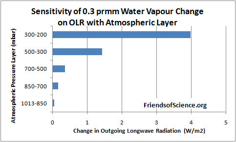
Dr. Ferenc Miskolczi performed computations using the HARTCODE line-by-line radiative code to determine the sensitivity of OLR to a 0.3 mm change in precipitable water vapor in each of 5 layers of the NVAP-M project. The program uses thousands of measured absorption lines and is capable of doing accurate radiative flux calculations. Figure 2 shows the effect on OLR of a change of 0.3 mm in each layer.
The results show that a water vapor change in the 500-300 mb layer has 29 times the effect on OLR than the same change in the 1013-850 mb near-surface layer. A water vapor change in the 300-200 mb layer has 81 times the effect on OLR than the same change in the 1013-850 mb near-surface layer.

Figure 2. Sensitivity of 0.3 mm precipitable water vapor change on outgoing longwave radiation by atmospheric layer.
Table 2 below shows the change in OLR per change in water vapor in each layer, and the change in OLR from 1990 to 2001 due to the change in precipitable water vapor (PWV).
| L1 | L2 | L3 | Sum | CO2 | ||
| OLR/PWV | W/m2/mm | -0.329 | -1.192 | -4.75 | ||
| OLR/CO2 | W/m2/ppmv | -0.0101 | ||||
| OLR change | W/m2 | -0.569 | 0.679 | 2.613 | 2.723 | -0.171 |
Table 2. Change of OLR by layer from water vapor and from CO2 from 1990 to 2001.
The calculations show that the cooling effect of the water vapor changes on OLR is 16 times greater than the warming effect of CO2 during this 11-year period. The cooling effect of the two upper layers is 5.8 times greater than the warming effect of the lowest layer.
These results highlight the fact that changes in the total water vapor column, from surface to the top of the atmosphere, is of little relevance to climate change because the sensitivity of OLR to water vapor changes in the upper atmosphere overwhelms changes in the lower atmosphere.
The precipitable water vapour by layer versus latitude by one degree bands for the year 1991 is shown in Figure 3. The North Pole is at the right side of the figure. The water vapor amount in the Arctic in the 500 to 300 mb layer goes to a minimum of 0.53 mm at 68.5 degrees North, then increases to 0.94 mm near the North Pole.

Figure 3. Precipitable water vapor by layer in 1991.
The NVAP-M project extends the analysis to 2009 and reprocesses the Heritage NVAP data. This layered data is not publicly available. The total precipitable water (TPW) data is shown in Figure 4, reproduced from the paper Vonder Haar et al (2012) here. There is no evidence of increasing water vapor to enhance the small warming effect from CO2.

Figure 4. Global month total precipitable water vapor NVAP-M.
The Radiosonde Data
Water vapor humidity data is measured by radiosonde (on weather balloons) and by satellites. The radiosonde humidity data is from the NOAA Earth System Research Laboratory here.

Figure 5. Global relative humidity, middle and upper atmosphere, from radiosonde data, NOAA Earth System Research Laboratory.
A graph of the global average annual relative humidity (RH) from 300 mb to 700 mb is shown in Figure 5. The specific humidity in g/kg of moist air at 400 mb (8 km) is shown in Figure 6. It shows that specific humidity has declined by 14% since 1948 using the best fit line.

Figure 6. Specific humidity at 400 mb pressure level
In contrast, climate models all show RH staying constant, implying that specific humidity is forecast to increase with warming. So climate models show positive feedback and rising specific humidity with warming in the upper troposphere, but the data shows falling specific humidity and negative feedback.
Many climate scientists dismiss the radiosonde data because of changing instrumentation and the declining humidity conflicts with the climate model simulations. However, the radiosonde instruments were calibrated and the data corrected for changes in response times. The data before 1960 should be regarded as unreliable due to poor global coverage and inferior instruments. The near surface radiosonde measurements from 1960 to date show no change in relative humidity which is consistent with theory. Both the satellite and radiosonde data shows declining upper atmosphere humidity, so there is no reason to dismiss the radiosonde data. The radiosonde data only measures humidity over land stations, so it is interesting to compare to the satellite measurements which have global coverage.
Comparison Between Radiosonde and Satellite Data
The specific humidity radiosonde data was converted to precipitable water vapor for comparison with the satellite data. Figure 7 compares the satellite data to the radiosonde data for the years 1988 to 2001.

Figure 7. Comparison between NOAA radiosonde and NVAP satellite derived precipitable water vapor.
The NOAA and NVAP data compares very well for the period 1988 to 1995. The NVAP satellite data shows less water vapor in the upper and middle layers than the NOAA data. In 2000 and 2001 the NVAP data shows more water vapor in the near-surface layer than the NOAA data. The vertical change on the logarithmic graph is roughly equal to the forcing effect of each layer, so the NVAP data shows water vapor has a greater cooling effect than the radiosonde data.
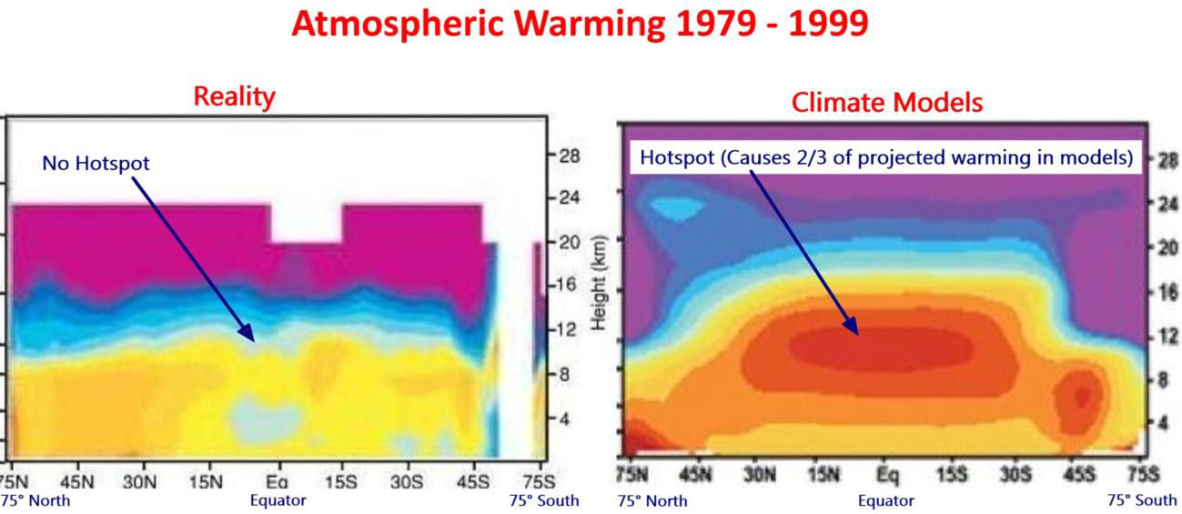
The Tropical Hot Spot
The models predict a distinctive pattern of warming – a “hot-spot” of enhanced warming in the upper atmosphere at 8 km to 13 km over the tropics, shown as the large red spot in Figure 8. The temperature at this “hot-spot” is projected to increase at a rate of two to three times faster than at the surface. However, the Hadley Centre’s real-world plot of radiosonde temperature observations from weather balloons shown below does not show the projected hot-spot at all. The predicted hot-spot is entirely absent from the observational record. If it was there it would have been easily detected.
The hot-spot is forecast in climate models due to the theory that the water vapor profile in the tropics is dominated by the moist adiabatic lapse rate, which requires that water vapor increases in the upper atmosphere with warming. The moist adiabatic lapse rate describes how the temperature of a parcel of water-saturated air changes as it move up in the atmosphere by convection such as within a thunder cloud. A graph here shows two lapse rate profiles with a larger temperature difference in the upper atmosphere than at the surface. The projected water vapor increase creates the hot-spot and is responsible for half to two-thirds of the surface warming in the IPCC climate models.

Figure 8. Climate models predict a hot spot of enhanced warming rate in the tropics, 8 km to 13 km altitude. Radiosonde data shows the hot spot does not exist. Red indicates the fastest warming rate. Source: http://joannenova.com.au
The projected upper atmosphere water vapor trends and temperature amplification at the hot-spot are intricately linked in the IPCC climate theory. The declining upper atmosphere humidity is consistent with the lack of a tropical hot spot, and both observations prove that the IPCC climate theory is wrong.
A recent technical paper Po-Chedley and Fu (2012) here compares the temperature trends of the lower and upper troposphere in the tropics from satellite data to the climate model projections from the period 1981 to 2008.2 The upper troposphere is the part of the atmosphere where the pressure ranges from 500 mb to 100 mb, or from about 6 km to 15 km. The paper reports that the warming trend during 1981 to 2008 in the upper troposphere simulated by climate models is 1.19 times the simulated warming trend of the lower atmosphere in the tropics. (Note this comparison is to the lower atmosphere, not the surface, and includes 10 years of no warming to 2008.) Using the most current version (5.5) of the satellite temperature data from the University of Alabama in Huntsville (UAH), the warming trend of the upper troposphere is only 0.973 of the lower troposphere in the tropics for the same period. This is different from that reported in the paper because the authors used an obsolete version (5.4) of the data. The satellite data shows not only a lack of a hot-spot, it shows a cold-spot just where a hot-spot was predicted.
Conclusion
Climate models predict upper atmosphere moistening which triples the greenhouse effect from man-made carbon dioxide emissions. The new satellite data from the NASA water vapor project shows declining upper atmosphere water vapor during the period 1988 to 2001. It is the best available data for water vapor because it has global coverage. Calculations by a line-by-line radiative code show that upper atmosphere water vapor changes at 500 mb to 300 mb have 29 times greater effect on OLR and temperatures than the same change near the surface. The cooling effect of the water vapor changes on OLR is 16 times greater than the warming effect of CO2 during the 1990 to 2001 period. Radiosonde data shows that upper atmosphere water vapor declines with warming. The IPCC dismisses the radiosonde data as the decline is inconsistent with theory. During the 1990 to 2001 period, upper atmosphere water vapor from satellite data declines more than that from radiosonde data, so there is no reason to dismiss the radiosonde data. Changes in water vapor are linked to temperature trends in the upper atmosphere. Both satellite data and radiosonde data confirm the absence of any tropical upper atmosphere temperature amplification, contrary to IPCC theory. Four independent data sets demonstrate that the IPCC theory is wrong. CO2 does not cause significant global warming.
Note 1. The NVAP data in Excel format is here.
Note 2. The lower troposphere data is: http://www.nsstc.uah.edu/public/msu/t2lt/uahncdc.lt
The upper troposphere data is calculated as 1.1 x middle troposphere – 0.1 x lower stratosphere; where middle troposphere is: http://www.nsstc.uah.edu/public/msu/t2/uahncdc.mt and the lower stratosphere is:http://www.nsstc.uah.edu/public/msu/t4/uahncdc.ls
============================================================
The original article is located at http://www.friendsofscience.org/index.php?id=483
Willis and Bill Illis,
The “effective emissivity” need not be related to material properties. Consider the steel greenhouse. If you relate the power P radiated to the inner surface temperature T it is exactly
P = 0.5*σ*T^4.
But all surfaces are black.
If you divide the increment formula
dP = 4*ε*σ*T^3 dT
by the first relation P = ε*σ*T^4
you get simply
dP/P = 4*dT/T
or dT=(T/4/P) dP = (287/4/238)*3.7 = 1.12°C
That form makes it clear that the only info used are the present OLR, T and the 4, which reflects the T^4 behaviour.
Willis, the reason for using 238 is that that is the thermal IR flux, and as such is the one S-B would relate to the surface temperature T. The flux of 340 W/m2 includes the reflected sunlight; re-radiation of that SW component does not depend on T.
Very interesting. Thanks.
It also makes the cause of the late 20th century warming clear. Increased surface solar insolation from decreased clouds.
a result that is sixteen times as large as a lie is just a bigger lie…
Willis, please see Clive Best comment at: March 7, 2013 at 4:33 am
This is a good explanation of the 1.1 C no-feedback temperature change due to doubled CO2.
Your wrote:
The global averaged incoming shortwave radiation is 341 W/2, from the TFK2009 energy balance diagram here:
http://www.friendsofscience.org/assets/documents/FOS%20Essay/TFK2009.jpg
About 30% is reflected direct back to space, so it does not enter the climate system and has no effect on the longwave radiation emitted by the earth to space. The diagram shows 239 W/m2 outgoing longwave radiation (OLR) emitted to space. If you add back in the fantasy net absorbed 1 W/m2, the OLR to space is 240 W/m2, which is the number Clive Best used. The diagram shows the atmosphere absorbed 78 W/m2 plus the surface absorbed 161 W/m2 is the total absorbed shortwave radiation of 239 W/m2. The OLR equals the shortwave absorbed radiation, which is the incoming solar X (1- albedo).
Albedo = 1 – 239/340 = 29.7%
Nick Stokes says:
March 7, 2013 at 12:46 pm
Thanks, Nick. I understand that you can mash together separate variables. But when you do so, you destroy any claim that what remains is either emissivity or the S-B equation. The result, as you seem to agree, is that what you are calling “effective emissivity” has no physical meaning. You can do it … but it’s not emissivity of any type after you do it.
Instead, it is an amalgam of the S-B equation, multiplied by the efficiency of the climate system at concentrating energy at the surface. Mathematically, it works. Theoretically, it confuses things.
You’ve already said that your amalgam has no physical meaning. You can’t then base your argument on physical meaning.
The formula you give is simply S-B time efficiency. The efficiency needs to be treated as the separate variable which it is. The question is solely how to measure the efficiency of the entire planet-wide climate system. The efficiency of any system is related to total incoming energy. Losses of any kind, whether reflective, sensible heat, latent heat, or direct radiation to space, are all part of that whole system.
Next, you make this most far-reaching profound mistake:
I see this mistake made all the time. It is the mistake of not looking at the climate system with the eye of an engineer. An engineer knows that in the climate system, the clouds control the amount of incoming radiation, and further that they actively oppose any temperature increase—tropical clouds increase with temperature. As a result, the re-radiation of that SW component absolutely depends on T.
Nor is this simply theory. I’ve demonstrated this quite convincingly using the TAO buoy dataset. I’ve demonstrated the same thing using satellite photos of the Pacific. And I’ve demonstrated it using the CERES dataset to show that on a net basis clouds warm the earth in winter and cool it in summer. Both the occurrence and the nature of tropical clouds is not only a function of T, it is a wildly non-linear function of T. The tropical temperature versus albedo curve has “knuckles”, bends at each of the threshold temperatures for cumulus and cumulonimbus formation.
You can’t just ignore all that huge part of the climate system. It’s not somehow separate. It is an integral part of the whole.
The planet receives 340 W/m2 from the sun. That has to be the starting point for any climate system efficiency analysis, because that is the total energy available to the system. The fact that it only uses part of the available energy is an integral feature of the temperature control system, not something where you can incorrectly claim it’s a constant, doesn’t depend on T, and then ignore it. The albedo changes from changes in clouds and ice and ground cover are part of the system, and all of those are functions of the temperature.
You have to start with all the available energy when you’re looking at the whole system. You can’t just restrict yourself to one kind of energy, say longwave IR. We’re talking about the global, full analysis, the entire climate system.
There is also a further mistake, which is confusing equilibrium conditions with the energy expended to achieve those conditions … but that’s a whole separate post. Briefly, far from equilibrium, variations in forcing make more difference than at equilibrium. But like I say that’s for another time.
w.
Ken Gregory says:
March 7, 2013 at 1:10 pm
Thanks, Ken. Unfortunately, Clive’s explanation contains more holes than solid floor. Going by way of some imagined “blackbody temperature” is fraught with pitfalls and precarious assumptions.
However, I do clearly understand Nick’s explanation … and I think you’re making the same mistake he makes. You can’t just ignore part of the energy flow by pretending it’s a constant. It’s not, it’s far, far from a constant. Please reconsider your position in light of my preceding post.
All the best,
w.
Willis,
This 1.12°C is just a concept number. If you add 3.7 W/m2, you expect the system to get warmer. How much warmer? So they start with the simplest possible quantification, and then start to think about possible added feedbacks.
The dependence of albedo on temperature is one of those feedbacks – a cloud feedback. It’s not something you try to include at this first stage. What numbers could you use to express it?
All this reasoning really says is that we have a known state, 238 W/m2 and 287°K, and we expect small changes to that to follow a T^4 rule. If you include albedo SW in the arithmetic, that implies that it too follows a T^4 rule. Now it may not be constant, but T^4 is not justified for SW.
Willis,
Look back at the Earth from the moon. What temperature do you measure ?
255K right .
Double CO2. Now what temperature do you see ?
255K again.
Did anything change ?
Well yes the atmosphere readjusted slightly to maximise heat transfer from the surface. This post provides evidence that the H2O profile adjusts to restore radiative heat loss from the surface rather than the simple BB feedback.
Otherwise Nick Stokes or my simple argument equally apply
Nick Stokes says:
March 7, 2013 at 2:20 pm
Thanks for the response, Nick. Two you advance two lines of thought there.
First, you say It’s just a “concept number” … sorry, this is a science blog, and I truly don’t have a clue what you mean by a “concept number”. Mosh and you have advanced it as a mathematically derivable fact … are you and he in agreement on this retraction? What does “concept number” mean?
Second, that’s not the “simplest possible quantification”. The simplest one uses a directly measurable quantity, 340 W/m2 from the sun. Instead, you propose using that measured number multiplied by one minus an imperfectly measured albedo … under what rubric is that “simpler”?
You guys are the ones claiming that this magical number applies to the whole climate system … and then leaving out the entire temperature control system out of your analysis. If you’re choose to describe only part of the whole, then why haven’t you highlighted that fact? And how can you claim it has global application, or any application, in that case? You’re describing how the system would work if you cut it in half … so what?
No, 340 W/m2 downwelling solar radiation at the top of the atmosphere is the known state. 238 W/m2 is a calculated value measuring the result of the action of the cloud-based temperature control system that keeps the planet from overheating.
Depends entirely on your unspecified “arithmetic”, so I couldn’t say. That wouldn’t happen in my arithmetic, for example, it doesn’t imply a T^4 dependence.
I’ve already said (and given an example and illustrative theoretical curves and explanation and demonstrated elsewhere) that the relationship between albedo and temperature is non-linear, with “knuckles” at threshold temperatures. So no … it’s not T^4 based. Instead, what changes is how much time in a given day/month/year we spend in each of the different temperature regimes. When it’s hot, a fully formed cumulus field forms earlier in the day, and when it’s cool, it forms later in the day. And that is one of the major systems regulating the temperature, and preventing overheating.
People are all worried about overheating from CO2 … well, consider overheating from the extra eighty watts per square metre that the clouds control. If those jokers joined the Union and went on strike, we’d fry in a month. Heck, if they just changed the average albedo from 30% to 31%, that would balance out the entire doubling of CO2 … and they do that and more all the time.
And remember that to do that, they just have to shift the onset time slightly. A half-hour shift in the onset time of cumulus formation around mid-day makes a 24/7 average change of about 10 W/m2. This system will easily counteract the 3.7 W/m2 of additional CO2 forcing from a doubling … all it will take is a few minutes earlier onset time, and the balance is restored.
You can’t just leave that entire complex system out of any calculations or claims that you say are global in nature. That cloud-based control of the amount of incoming energy is an integral part of the climate system. It cannot be arbitrarily “plucked out” just so you can simplify your calculations. That just leads you to false conclusions.
w.
Very interesting. This fits very well with what I have been saying for a few years. We have a warming effect of CO2 (called the GHE) and we also have a cooling effect due to CO2 as follows. The additional CO2 in the atmosphere increases the radiation of energy from the atmosphere to space. This is predominant in the upper atmosphere because there is much less water vapor.
It’s only natural that a cooler upper atmosphere will shed water vapor due to condensation. So, the H2O works as a positive feedback on the cooling effect in the upper atmosphere just like it works as a positive feedback on the GHE in the lower atmosphere.
Imagine that, nature in balance.
Willis,
“Mosh and you have advanced it as a mathematically derivable fact …”
Well, it’s mathematically derivable – I gave the derivation. But Mosh said it was a
“sensitivity to forcing without feedbacks”
Now the real world has feedbacks, so it isn’t a number you can measure experimentally. It just a concept that helps to figure stuff out. Like, say, a steel greenhouse.
“Instead, you propose using that measured number multiplied by one minus an imperfectly measured albedo “
OLR was once worked out that way. But it is now
directly measured by CERES, with excellent agreement.
“You guys are the ones claiming that this magical number applies to the whole climate system … and then leaving out the entire temperature control system out of your analysis.”
Well, I’d invite you to quote me there. As I said above, the 1.12°C is a starting point (“forcing without feedbacks”). Then you think about feedbacks.
“Depends entirely on your unspecified “arithmetic”, so I couldn’t say.”
No, it’s specified. dP=(P/4/T) dT. P=238,T=287. It comes from differentiating P = const*T^4.
“That just leads you to false conclusions.”
It isn’t a conclusion. It’s a starting point.
phlogiston says: March 6, 2013 at 11:53 pm
‘Talking of camels, I came across this at the BBC….’
Yes but it seems like many others it was a rehash of this original media report-
http://news.nationalpost.com/2013/03/05/giant-ancient-camel-remains-discovered-in-canadian-arctic/
and note that priceless throwaway line from another ‘earth scientist’ –
“The camel is an ambassador for climate change,”
Where is Josh to knock us up some T-Shirt logos headed- ‘Arctic Camel’ with a nice toon pic of our iconic camel underneath and then below that-
‘I survived global warming, climate change, climate disruption and I’ll damn well outlive Big Climate and their extreme weather!’
Sara Hindle says:
March 6, 2013 at 11:33 am
Why does the upper atmosphere satellite data humidity decline after 1995 more than the radiosonde humidity data? Is there some reason upper atmosphere humidity would decline more over the oceans than over land?
The greater decline in the SH also points to an oceanic effect. Assuming the warming over recent decades isn’t spurious, ocean evaporation must have increased. Which means precipitation efficiency has increased also.
I’d point to decreased cloud seeding aerosols = reduction in more persistent clouds, and hence more precipitation. But I’d expect this more over land than oceans. So, a bigger reduction over the oceans is a puzzle. As mentioned above I’d look to a biological mechanism. Perhaps, cloud seeding bacteria originating in the oceans have increased for some reason.
Nick Stokes says:
March 7, 2013 at 4:00 pm
Thanks as always for your interesting and detailed answers, Nick, much appreciated.
Regarding this first point, that’s my issue exactly. It is the sensitivity of the system if you ignore half the system … I fear that claiming anything but curiosity value for the result is a bridge too far.
The difficulty is that you are not just ignoring feedbacks. In addition to feedbacks, you are ignoring the active climate control system that keeps the planet from overheating. And when you ignore that, I’m sorry, but your results are meaningless. You can’t just chop the control system off of a complex set of interactions, how does that help you understand anything?
You missed my point, likely I wasn’t clear. You’d said that you were going for the simplest system. I said your proposed alternative is no simpler than just using TSI. It’s more complex, because it contains an additional variable (that you are unfortunately treating as a constant, but that’s another issue). The question was your claim of simplicity for using 238 W/m2. Using TSI alone is simpler than TSI * (1 – albedo). Minor point though.
It’s the lack of quotes that is telling. You say that for the whole system without feedbacks, the value is X.
But you haven’t taken out just the feedbacks. You’ve also removed the natural system that controls the temperature. That’s the part that is never acknowledged, that your system is one without both feedbacks and active temperature control.
No, now you’ve specified it. Before, it could have been any arithmetic, I can’t read your mind, so thanks for the specificity.
However, your assumption is only true after you’ve conflated the efficiency of the climate system with the emissivity to make what you agree is a non-physical number. Break the efficiency back out of the S-B equation before differentiation. This is the kind of trouble I talked about getting into by mixing the two up.
The efficiency of the overall system, whether you start at 238 W/m2 or do it properly by starting at 340 W/m2, is a complex function in its own right. It is not a constant by any means. Nor does it have much to do with emissivity. Instead it is ruled by the huge parasitic losses in the system, from direct radiation to space, sensible heat, latent heat, and evapotranspiration. All of these act to oppose increases in temperature.
When you pull it back out of the S-B equation, you see that the “arithmetic” is incorrect. When you differentiate the equation, you have to differentiate the efficiency separately. It’s not a constant, it’s a complex formula all it’s own. It doesn’t belong inside the S-B equation, that’s why it’s not proportional to T^4, and more to the point why we don’t expect it to be.
I list one such conclusion immediately above.
Next, let us assume that your way of calculation (starting at 238 W/m2) is for the system without feedback. I’ve shown above that you’ve removed more than that, but lets assume you are correct. Additionally, lets assume that my way of calculation (starting at 340 W/m2 and thus including everything) is for the complete system with all conceivable feedbacks.
With that as a basis, the sensitivity without feedbacks per the calculations is 1.2°C per doubling of CO2.
And the sensitivity with all feedbacks is 0.8°C per doubling … tells you something about whether positive or negative feedbacks dominate, right?
Finally, be clear. None of this tells us what’s going on at equilibrium. In a governed system, the sensitivity at equilibrium is basically zero, because the control phenomena (primarily clouds and thunderstorms) are temperature-threshold based, not forcing-based, and are governed by the laws of wind, wave, temperature, and cloud formation—and NOT by the amount of power available. We always have 80W/m2 of additional power available to the system, and that fact alone should make it clear that the amount of energy (forcing) is not the determinant of temperature. The natural system itself actively regulates the energy input to prevent either overheating or overcooling.
w.
Ken Gregory says:
It is not the best available data. It is data that the providers of the data tell you explicitly is not suited for the purpose that you are using it for. Furthermore:
(1) These results are in contradiction with other satellite data looking at the upper tropospheric humidity trends, such as that discussed here: http://www.sciencemag.org/content/310/5749/841.abstract
(2) These results would have you believe that the multidecadal trends in response to warming are completely different from the shorter term fluctuations in response to warming, since the data unambiguously show that the water vapor feedback is operating as expected (i.e., the upper atmosphere is moistening when temperatures increase) for the shorter term fluctuations in temperature (e.g., on monthly to yearly timescales).
So, in summary,
(a) Very basic physics tells us that the atmosphere will moisten as the temperature warms.
(b) The data very unambiguously show that this is the case for temperature fluctuations on monthly- to yearly-timescales.
(c) For longer term multidecadal trends, most of the satellite and radiosonde/re-analysis data sets also show this behavior. However, there is one radiosonde/re-analysis data set and one satellite data set that show otherwise. Yet, you have clung onto these and neglected all of the other data that yields different conclusions even though there are very good reasons to believe that the data sets you are looking at have severe problems (e.g., http://geotest.tamu.edu/userfiles/216/Dessler10.pdf ), and in fact, the very producers of the data set have explicitly warned that the data is not suited for the purpose of studying multidecadal trends.
Richard M says:
While it is true that the stratosphere is expected and observed to cool as greenhouse gases increases, what we are talking about here is the upper troposphere, which is expected and observed to warm.
Actually what you’re talking about is a calculated Upper Troposhere, not actual measurements from the Upper Troposphere. You gotta read the fine print!
Ken Gregory, your images for Figure 8 are decptive. The one showing the model forecast is for between 1958 – 1999. The one for observations is for 1979-1999. You’ve labelled them both as 1979-1999.
Willis Eschenbach says:
March 7, 2013 at 1:52 pm
Clive and Nick were discussing the no-feedback sensitivity to CO2. The no-feedback sensitivity by definition is the theoretical temperature response to double CO2 where albedo, water vapor, clouds, lapse rate, evaporation are constant. We are not pretending albedo is a constant; albedo IS constant BY definition of no-feedback sensitivity. Your preceding post talks about changing clouds, which is irrelevant to a no-feedback calculation.
Does the no-feedback climate sensitivity tell us anything about the actual climate sensitivity? NOPE! I mentioned it in the lead post only to point out that a large part of climate model projected temperature rise is due to projected rising upper atmosphere water vapor.
joeldshore says:
March 7, 2013 at 5:45 pm
While it is true that the stratosphere is expected and observed to cool as greenhouse gases increases, what we are talking about here is the upper troposphere, which is expected and observed to warm.
That’s a bit dishonest Joel as no one can separate the effect of the oceans releasing heat from the effects of CO2. It could very well be the “observed” effects have been reduced by the CO2 radiating additional energy to space in the Troposphere. The lack of a hot spot is quite telling. You have no data that tells you otherwise. Why do you claim more knowledge than you possess?
joeldshore says:
March 7, 2013 at 5:42 pm
The NVAP team have done a great deal of work to create a global water vapor dataset by merging information from several different satellite instruments. Some instruments are better over land or with clouds, some better over oceans or clear-sky. The satellite data has been compared to in situ radiosonde measurements to check their accuracy. This is the first dataset that has global coverage and has data by layer.
I am aware of the NVAP Trend Statement. All datasets have potential for biases and can be improved. The Trend Statement says they are working to improved the data. I expect that the NVAP-M data will be better than the Heritage data, but it is not available, so it is of no use to me.
I provided a time series of the by layer Heritage NVAP data, and calculated the consequences to OLR of that data. The NVAP team also provided a times series of the NVAP-M data total water vapor column, presented as Figure 4 in my article. All datasets have limitations. That is why I discussed four datasets, two of humidity and two of temperature, all of which demonstrate that the climate model predicted hot-spot does not exist. You need to consider all available data. The IPCC and the media presents data favorable to their AGW agenda. I am presenting data that the IPCC will not present because it does not support their agenda.
This is a Soden et al 2005 paper, 7 1/2 years old. It uses the the High Resolution Infrared Radiometer Sounder (HIRS) 6.3 micro-meter water vapor band to estimate water vapor only in clear-sky, no clouds. Since clouds cover 60% of the earth, this is a serious restriction.
Yes, over short time periods, water vapor increases with temperature, but not over long term periods. That is why using a short-term event, like the Mt. Pinatubo eruption, to calculate climate sensitivity will give an overestimation. Here is a graph of upper atmosphere water vapor (400 mb) in the tropics versus temperature from radiosonde data.
http://www.friendsofscience.org/assets/documents/FOS%20Essay/SH400TropicsVsTemp.jpg
The graph is a phase space plot of the data points connected in time sequence. The annual data shows linear striations increasing from bottom left to top right, confirming that higher temperatures relate to higher specific humidity over short time intervals. But the overall trend is down, showing that the negative water vapor feedback is due to slower processes. This gives a very low R2 correlation factor of 0.016 for specific humidity vs temperature. Contrast this with a graph of specific humidity vs CO2:
http://www.friendsofscience.org/assets/documents/FOS%20Essay/SH400TropicsVsCO2.jpg
This R2 factor is a fantastic 0.729! More CO2 displaces water vapor.
James says:
March 7, 2013 at 7:41 pm
James, if you read the caption for Figure 8, you will see I did not make or label the graphs. The Figure is not labelled “Friends of Science” and the caption says Source: http://joannenova.com.au
If you have a reason to believe the model forecasts graph is for temperature trends from 1958 – 1999, you could provide a link to the original source. I suspect you are referring to this graph which is labeled 1958 – 1999:
http://jonova.s3.amazonaws.com/graphs/hot-spot/hot-spot-model-predicted.gif
This is different from the graph of Figure 8.
The surface temperature trend from 1958 – 1999 at 0.11 C/decade is not a lot different from the temperature trend from 1979 – 1999 at 0.15 C/decade from HadCrut3, so the modeled hot-spot temperature trends wouldn’t be a lot different anyway.
JamesS says:
March 6, 2013 at 12:59 pm
Alex, you must have missed the section below. It explains why a slight increase at near-ground levels is not as important as the decreases at higher levels.
The results show that a water vapor change in the 500-300 mb layer has 29 times the effect on OLR than the same change in the 1013-850 mb near-surface layer. A water vapor change in the 300-200 mb layer has 81 times the effect on OLR than the same change in the 1013-850 mb near-surface layer.
————————————————–
James, this is an interesting point that I don´t quite understand.
I always thought, the water vapor absorption is NOT saturated (CO2 is saturated). This means, the heating goes about linear with the vapor concentration (for CO2 it is log at the best).
Then, it is the total vapor in the column that counts.
In the water vapor absorption band, the IR can leave the earth surface directly (partially).
In the CO2 band, no radiation can leave surface and must be re-emitted until the band opens somewhere in tropopause…
May be, I miss some physics?
Ken says “If you have a reason to believe the model forecasts graph is for temperature trends from 1958 – 1999, you could provide a link to the original source.”
Ken, I am surprised that for someone claiming to be an expert you do not know the original source of the image you present! You’re the one presenting this information as if you know what you’re talkinig about.
What’s more, asking other people to seek out the original source in order to determine what period it covers is pathetic. You are the one drawing conclusions on this and it’s quite evident you are not familiar with the paper from which it comes.
If you knew your subject matter then you’d be well aware that the image you present, and the one from Nova’s site are from exactly the same source, on exactly the same page, in exactly the same figure and both represent 1958-1999.
It beggars belief that some people think posts on this blogger sites are conducted by experts. I am offended that you resort to such trickery in order to fool the unwary.
Willis, Nick, might I suggest that rather than just trying to outmath each other, try something like this: http://forecast.uchicago.edu/Projects/modtran.html, if each of you agreed on a couple parameter choices to compare, you would be able to directly illustrate the effects of clouds and CO2 doubling with regards to radiation leaving the atmosphere.
Now, I saw another comment above that said something to the effect of “in a no feedback assumption, albedo is constant”… that is an interesting claim, since albedo is never constant anywhere at the surface, nor is emissivity so easy to pin down.
We can average them roughly… but it’s not as simple as pointing a sensor at a calibration target and pointing it at the entire planet and saying “yep, that’s the albedo and here is the emissivity, to within a few significant digits”.