
Guest post submitted by Ken Gregory, Friends of Science.org
An analysis of NASA satellite data shows that water vapor, the most important greenhouse gas, has declined in the upper atmosphere causing a cooling effect that is 16 times greater than the warming effect from man-made greenhouse gas emissions during the period 1990 to 2001.
The world has spent over $ 1 trillion on climate change mitigation based on climate models that don’t work. They are notoriously poor at simulating the 20th century warming because they do not include natural causes of climate change – mainly due to the changing sun – and they grossly exaggerate the feedback effects of greenhouse gas emissions.
Most scientists agree that doubling the amount of carbon dioxide (CO2) in the atmosphere, which takes about 150 years, would theoretically warm the earth by one degree Celsius if there were no change in evaporation, the amount or distribution of water vapor and clouds. Climate models amplify the initial CO2 effect by a factor of three by assuming positive feedbacks from water vapor and clouds, for which there is little direct evidence. Most of the amplification by the climate models is due to an increase in upper atmosphere water vapor.
The Satellite Data
The NASA water vapor project (NVAP) uses multiple satellite sensors to create a standard climate dataset to measure long-term variability of global water vapor.
NASA recently released the Heritage NVAP data which gives water vapor measurement from 1988 to 2001 on a 1 degree by 1 degree grid, in three vertical layers.1 The NVAP-M project, which is not yet available, extends the analysis to 2009 and gives five vertical layers.
From the NVAP project page:
The NASA MEaSUREs program began in 2008 and has the goal of creating stable, community accepted Earth System Data Records (ESDRs) for a variety of geophysical time series. A reanalysis and extension of the NASA Water Vapor Project (NVAP), called NVAP-M is being performed as part of this program. When processing is complete, NVAP-M will span 1987-2010. Read about changes in the new version.
Water vapor content of an atmospheric layer is represented by the height in millimeters (mm) that would result from precipitating all the water vapor in a vertical column to liquid water. The near-surface layer is from the surface to where the atmospheric pressure is 700 millibar (mb), or about 3 km altitude. The middle layer is from 700 mb to 500 mb air pressure, or from 3 km to 6 km attitude. The upper layer is from 500 mb to 300 mb air pressure, or from 6 km to 10 km altitude.
The global annual average precipitable water vapor by atmospheric layer and by hemisphere from 1988 to 2001 is shown in Figure 1.
The graph is presented on a logarithmic scale so the vertical change of the curves approximately represents the forcing effect of the change. For a steady earth temperature, the amount of incoming solar energy absorbed by the climate system must be balanced by an equal amount of outgoing longwave radiation (OLR) at the top of the atmosphere. An increase of water vapor in the upper atmosphere would temporarily reduce the OLR, creating a forcing of more incoming than outgoing energy, which raises the temperature of the atmosphere until the balance is restored.

Figure 1. Precipitable water vapor by layer, global and by hemisphere.
The graph shows a significant percentage decline in upper and middle layer water vapor from 1995 to 2001. The near-surface layer shows a smaller percentage increase, but a larger absolute increase in water vapor than the other layers. The upper and middle layer water vapor decreases are greater in the Southern Hemisphere than in the Northern Hemisphere.
Table 1 below shows the precipitable water vapor for the three layers of the Heritage NVAP and the CO2 content for the years 1990 and 2001, and the change.
| Layer | L1 near-surface | L2 middle | L3 upper | Sum | CO2 |
| 1013-700 | 700-500 | 500-300 | |||
| mm | mm | mm | mm | ppmv | |
| 1990 | 18.99 | 4.6 | 1.49 | 25.08 | 354.16 |
| 2001 | 20.72 | 4.03 | 0.94 | 25.69 | 371.07 |
| change | 1.73 | -0.57 | -0.55 | 0.61 | 16.91 |
Table 1. Heritage NVAP 1990 and 2001 water vapour and CO2.
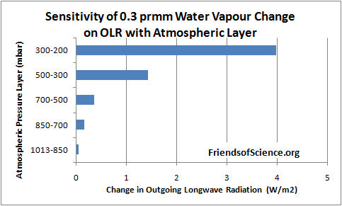
Dr. Ferenc Miskolczi performed computations using the HARTCODE line-by-line radiative code to determine the sensitivity of OLR to a 0.3 mm change in precipitable water vapor in each of 5 layers of the NVAP-M project. The program uses thousands of measured absorption lines and is capable of doing accurate radiative flux calculations. Figure 2 shows the effect on OLR of a change of 0.3 mm in each layer.
The results show that a water vapor change in the 500-300 mb layer has 29 times the effect on OLR than the same change in the 1013-850 mb near-surface layer. A water vapor change in the 300-200 mb layer has 81 times the effect on OLR than the same change in the 1013-850 mb near-surface layer.

Figure 2. Sensitivity of 0.3 mm precipitable water vapor change on outgoing longwave radiation by atmospheric layer.
Table 2 below shows the change in OLR per change in water vapor in each layer, and the change in OLR from 1990 to 2001 due to the change in precipitable water vapor (PWV).
| L1 | L2 | L3 | Sum | CO2 | ||
| OLR/PWV | W/m2/mm | -0.329 | -1.192 | -4.75 | ||
| OLR/CO2 | W/m2/ppmv | -0.0101 | ||||
| OLR change | W/m2 | -0.569 | 0.679 | 2.613 | 2.723 | -0.171 |
Table 2. Change of OLR by layer from water vapor and from CO2 from 1990 to 2001.
The calculations show that the cooling effect of the water vapor changes on OLR is 16 times greater than the warming effect of CO2 during this 11-year period. The cooling effect of the two upper layers is 5.8 times greater than the warming effect of the lowest layer.
These results highlight the fact that changes in the total water vapor column, from surface to the top of the atmosphere, is of little relevance to climate change because the sensitivity of OLR to water vapor changes in the upper atmosphere overwhelms changes in the lower atmosphere.
The precipitable water vapour by layer versus latitude by one degree bands for the year 1991 is shown in Figure 3. The North Pole is at the right side of the figure. The water vapor amount in the Arctic in the 500 to 300 mb layer goes to a minimum of 0.53 mm at 68.5 degrees North, then increases to 0.94 mm near the North Pole.

Figure 3. Precipitable water vapor by layer in 1991.
The NVAP-M project extends the analysis to 2009 and reprocesses the Heritage NVAP data. This layered data is not publicly available. The total precipitable water (TPW) data is shown in Figure 4, reproduced from the paper Vonder Haar et al (2012) here. There is no evidence of increasing water vapor to enhance the small warming effect from CO2.

Figure 4. Global month total precipitable water vapor NVAP-M.
The Radiosonde Data
Water vapor humidity data is measured by radiosonde (on weather balloons) and by satellites. The radiosonde humidity data is from the NOAA Earth System Research Laboratory here.

Figure 5. Global relative humidity, middle and upper atmosphere, from radiosonde data, NOAA Earth System Research Laboratory.
A graph of the global average annual relative humidity (RH) from 300 mb to 700 mb is shown in Figure 5. The specific humidity in g/kg of moist air at 400 mb (8 km) is shown in Figure 6. It shows that specific humidity has declined by 14% since 1948 using the best fit line.

Figure 6. Specific humidity at 400 mb pressure level
In contrast, climate models all show RH staying constant, implying that specific humidity is forecast to increase with warming. So climate models show positive feedback and rising specific humidity with warming in the upper troposphere, but the data shows falling specific humidity and negative feedback.
Many climate scientists dismiss the radiosonde data because of changing instrumentation and the declining humidity conflicts with the climate model simulations. However, the radiosonde instruments were calibrated and the data corrected for changes in response times. The data before 1960 should be regarded as unreliable due to poor global coverage and inferior instruments. The near surface radiosonde measurements from 1960 to date show no change in relative humidity which is consistent with theory. Both the satellite and radiosonde data shows declining upper atmosphere humidity, so there is no reason to dismiss the radiosonde data. The radiosonde data only measures humidity over land stations, so it is interesting to compare to the satellite measurements which have global coverage.
Comparison Between Radiosonde and Satellite Data
The specific humidity radiosonde data was converted to precipitable water vapor for comparison with the satellite data. Figure 7 compares the satellite data to the radiosonde data for the years 1988 to 2001.

Figure 7. Comparison between NOAA radiosonde and NVAP satellite derived precipitable water vapor.
The NOAA and NVAP data compares very well for the period 1988 to 1995. The NVAP satellite data shows less water vapor in the upper and middle layers than the NOAA data. In 2000 and 2001 the NVAP data shows more water vapor in the near-surface layer than the NOAA data. The vertical change on the logarithmic graph is roughly equal to the forcing effect of each layer, so the NVAP data shows water vapor has a greater cooling effect than the radiosonde data.
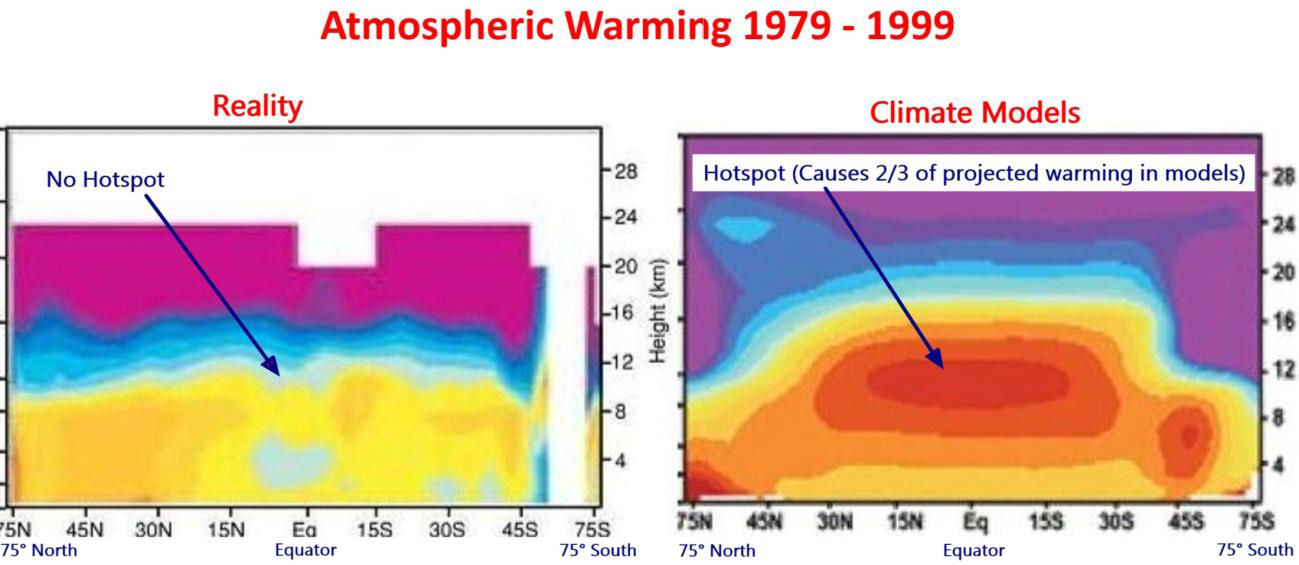
The Tropical Hot Spot
The models predict a distinctive pattern of warming – a “hot-spot” of enhanced warming in the upper atmosphere at 8 km to 13 km over the tropics, shown as the large red spot in Figure 8. The temperature at this “hot-spot” is projected to increase at a rate of two to three times faster than at the surface. However, the Hadley Centre’s real-world plot of radiosonde temperature observations from weather balloons shown below does not show the projected hot-spot at all. The predicted hot-spot is entirely absent from the observational record. If it was there it would have been easily detected.
The hot-spot is forecast in climate models due to the theory that the water vapor profile in the tropics is dominated by the moist adiabatic lapse rate, which requires that water vapor increases in the upper atmosphere with warming. The moist adiabatic lapse rate describes how the temperature of a parcel of water-saturated air changes as it move up in the atmosphere by convection such as within a thunder cloud. A graph here shows two lapse rate profiles with a larger temperature difference in the upper atmosphere than at the surface. The projected water vapor increase creates the hot-spot and is responsible for half to two-thirds of the surface warming in the IPCC climate models.

Figure 8. Climate models predict a hot spot of enhanced warming rate in the tropics, 8 km to 13 km altitude. Radiosonde data shows the hot spot does not exist. Red indicates the fastest warming rate. Source: http://joannenova.com.au
The projected upper atmosphere water vapor trends and temperature amplification at the hot-spot are intricately linked in the IPCC climate theory. The declining upper atmosphere humidity is consistent with the lack of a tropical hot spot, and both observations prove that the IPCC climate theory is wrong.
A recent technical paper Po-Chedley and Fu (2012) here compares the temperature trends of the lower and upper troposphere in the tropics from satellite data to the climate model projections from the period 1981 to 2008.2 The upper troposphere is the part of the atmosphere where the pressure ranges from 500 mb to 100 mb, or from about 6 km to 15 km. The paper reports that the warming trend during 1981 to 2008 in the upper troposphere simulated by climate models is 1.19 times the simulated warming trend of the lower atmosphere in the tropics. (Note this comparison is to the lower atmosphere, not the surface, and includes 10 years of no warming to 2008.) Using the most current version (5.5) of the satellite temperature data from the University of Alabama in Huntsville (UAH), the warming trend of the upper troposphere is only 0.973 of the lower troposphere in the tropics for the same period. This is different from that reported in the paper because the authors used an obsolete version (5.4) of the data. The satellite data shows not only a lack of a hot-spot, it shows a cold-spot just where a hot-spot was predicted.
Conclusion
Climate models predict upper atmosphere moistening which triples the greenhouse effect from man-made carbon dioxide emissions. The new satellite data from the NASA water vapor project shows declining upper atmosphere water vapor during the period 1988 to 2001. It is the best available data for water vapor because it has global coverage. Calculations by a line-by-line radiative code show that upper atmosphere water vapor changes at 500 mb to 300 mb have 29 times greater effect on OLR and temperatures than the same change near the surface. The cooling effect of the water vapor changes on OLR is 16 times greater than the warming effect of CO2 during the 1990 to 2001 period. Radiosonde data shows that upper atmosphere water vapor declines with warming. The IPCC dismisses the radiosonde data as the decline is inconsistent with theory. During the 1990 to 2001 period, upper atmosphere water vapor from satellite data declines more than that from radiosonde data, so there is no reason to dismiss the radiosonde data. Changes in water vapor are linked to temperature trends in the upper atmosphere. Both satellite data and radiosonde data confirm the absence of any tropical upper atmosphere temperature amplification, contrary to IPCC theory. Four independent data sets demonstrate that the IPCC theory is wrong. CO2 does not cause significant global warming.
Note 1. The NVAP data in Excel format is here.
Note 2. The lower troposphere data is: http://www.nsstc.uah.edu/public/msu/t2lt/uahncdc.lt
The upper troposphere data is calculated as 1.1 x middle troposphere – 0.1 x lower stratosphere; where middle troposphere is: http://www.nsstc.uah.edu/public/msu/t2/uahncdc.mt and the lower stratosphere is:http://www.nsstc.uah.edu/public/msu/t4/uahncdc.ls
============================================================
The original article is located at http://www.friendsofscience.org/index.php?id=483
Ken Gregory, I notice on that interesting graphic that the SE Asian monsoon is putting one huge belch of water way up every year. So much so, that it reaches, or exceeds, the maximum on the color-scale. [I remember the rainfall statistics for Cherrapunji from my high-school atlas!]
Are the numbers available for that gridded data, and can the demo be made to run slowly enough that I can take a better look as it changes during a single year?
Thanks, m
ut Richard says:
March 6, 2013 at 11:15 am
“Most scientists agree that doubling the amount of carbon dioxide (CO2) in the atmosphere, which takes about 150 years, would theoretically warm the earth by one degree Celsius if there were no change in evaporation”
Why? are they really sure?
###########################
read the text. See the reference to HARTCORT?
HARTCORT is one of the many validated, field tested, LBL radiation transfer codes.
What is a Radiation transfer code? That is a tested, validiated model used to predict how
radiation propagates through gases and particles. These models have their roots in the
work down by the department of defense. Why? suppose you want to calculate how far a
radar can see through the atmosphere. What you do is run radiation transfer codes and you
find out how much of the energy is transmitted, how much is absorbed, and how much is reflected by the atmosphere. These models rely on a huge database of physical data called HITRAN. That database was created by the air force.
If you are designing a radar or an IR missile or a plane that is supposed to be stealthy, you are required by contract to design the device using these codes. And then your predictions are tested.
These models are used when you estimate land surface temperature from a satellite. Basically if your engineering job is to figure out how radiation ( light, radar, lasers, any EM) transfers through the atmosphere, you use these codes. They are tested. They work. We rely on them for weather satellite images, radar engineering, IR engineering, IR astronomy.
The answer to “what happens if you double the water content in the air” can be answered by applying these codes. And then you can test that by doing field experiments with different amounts of water in the air, for example. Like doing tests in antarctica where the atmosphere is more dry. The coes allow you to predict how visible a IR target will be under different atmopsheric conditions.. like clouds or haze.. or changes for different parts of the world, deserts, tropics.. etc.
Hopefully you get the picture. These codes are working science. without them you cant build satellites that work, radars than work, IR detectors. Yes they are models. Like F=MA is a model of how things work.
The estimate for what happens of you double C02 comes from two numbers.
1. The increased Watts for doubling.
2. The sensitivity to forcing with and without feedbacks
#1. when you double c02 from 280 to 560, the radiation transfer codes predict 3.7 More
watts of forcing. If you want to doubt that number, you can collect a nobel prize by proving that the models are wrong. They are used every day by engineers. they are valididated. Knock yourself out. For reference, Lindzen, Christy, Spencer, Michaels, all credible skeptics buy this number. Sky dragons do not. They are wrong.
#2. The sensitivity to forcing without feedbacks means the 3.7Watts produces a 1.2C change
The argument is over whether feedbacks are positive or negative.
Assuming no feedbacks you get 1.2C per doubling.
Assume Positive feedbacks and this number can be as high as 6C
Assume negative feedbacks.. you get numbers less than 1.2C
now of course people dont just assume positive or negative feedbacks, they present arguments.
skeptics, like lindzen, presents arguments for negative feedbacks, consensus science argues for positive feedbacks. But both agree that.
” If everything else is held constant, doubling C02 will get you around 1.2C of warming.”
That’s why the real science argument is not over #1 ( more c02 is more forcing) but rather
over number #2. are feedbacks ‘equal” ( 1.2C) negative ( less than 1.2C) or positive ( >1.2c)
If you know nothing, your best guess is 1.2C Plus or minus “something” and the minus something cannot be that big, for paleo reasons.
As I had mentioned in previous comments, part of the reason for the fall in upper atmosphere humidity may be due to instrument and calibration issues. I am simply reporting the data and results. I don’t think the OLR change due to the reduction in upper atmosphere humidity can be so much greater than the OLR change due to CO2 increases over longer time periods. We will have to wait on the NVAP-M results.
G. Karst says:
March 6, 2013 at 9:02 pm
The total column humidity changed by +0.61 mm in 11 years, or by 0.055 mm/year on average, if you take the measurements at face value. The global average rainfall is 990 mm/year. So the change in total column humidity might cause a 0.0056% change in rainfall. Not something to worry about.
@Steven Mosher says on March 6, 2013 at 9:54 pm
Steven, do you have a reference for that? I thought that surface temperature was estimated using radiometers. See Estimating near-surface air temperature with NOAA AVHRR (Riddering and Queen, 2006), page 3 of the pdf:
There does not appear to be any overt reference to either HARTCORT OR HITRAN. Maybe the reference to them is implicit, but, if so, I would appreciate a reference or other explanation. Thanks.
Uh, how do you get that the negative feedbacks can not be that big from paleological arguments?
The last half a billion years have seen the planet remain between 10 and 20 Celsius on average over periods of millions of years at a time, barring the brief excursion at the Permian-Triassic boundary.
As for the dragons, some of them go a bit overboard, but some like Postma bring up rather convincing points upon examination. Myself, I remain unconvinced that radiative processes are as dominant in the determination of the surface temperature as they are presented. Infrared up/down is a result of the surface/atmosphere temperature, not the cause of it, and observing that there is IR bouncing around in the atmosphere doesn’t make it an energy source.
You might want to add that the 3.7 W/m^2 forcing is not independent of other assumptions, the surface temperature, height of the atmosphere, presence of water vapor, changes in pressure from the surface to the tropopause, stratospheric inversions due to ozone heated by the sun, and so on are all assumed to be at certain standard values in the radiative transfer codes.
The location itself is also important when making such calculations, but heck, don’t take my word for it.
http://forecast.uchicago.edu/Projects/modtran.html
Go play with the modtran codes yourself.
Trends in tropospheric humidity from reanalysis systems
A. E. Dessler1 and S. M. Davis2,3
JOURNAL OF GEOPHYSICAL RESEARCH, VOL. 115, D19127, doi:10.1029/2010JD014192, 2010
Based on the available evidence, it is our judgment
that negative trends in the tropical mid and upper troposphere
in response to long‐term climate change are spurious.
So, the data did get “reanalyzed” and the above judgement is the basis for throwing out any analysis using such data. The one and ONLY justification. Amazing.
observa says:
March 6, 2013 at 6:51 pm
I was going to suggest if the extreme weather catastrophists have coopted the polar bear as their iconic symbol, climate realists adopt the intrepid camel as ours. Our ship of the science desert.
Talking of camels, I came across this at the BBC – it is well established that camels evolved in north America, but now it turns out that their peculiar adaptations suiting them to desert life might first have arisen as adaptaions to cold and a near-Arctic habitat:
http://www.bbc.co.uk/news/science-environment-21673940
I’m not understanding why this isn’t a huge, huge story. Is there some other side to this I’m not aware of, some doubt or question about the data or the radiative physics? Because, on the face of it, it seems like it just strangles CAGW in the crib. Without a positive water vapor feedback, what is there to justify any concern about CO2 warming potential?
Okay, I guess this remark answers part of my question:
“the authors of the NVAP-M dataset do not think their data can be used for trend analysis.”
What I’d like to know is why is this data reliable for seasonal analysis, but not longer term trend analysis? Is it not properly calibrated? Or is it that the result of trend analysis is too embarrassing to the climate science community, and therefore has to be ignored or dismissed as insignificant one way or another?
Steven Mosher says:
March 6, 2013 at 9:54 pm
Not sure how you get that number, Steven, perhaps you could explain.
Let’s assume that the average surface temperature is say 14°C. If we assume an emissivity of 1 (blackbody), this gives us a Stefan-Boltzmann radiation of 385.5 W/m2.
Now, let’s suppose we add your claimed 1.2C to the temperature, giving us 15.2°C. The Stefan-Boltzmann radiation corresponding to that is 392 W/m2 …
This means it takes 6.5 W/m2 to raise the surface temperature by 1.2°C.
However, this is at the surface, not the TOA (top of atmosphere) where the change in forcing of 3.7 W/m2 is measured.
So we have to increase the 3.7 W/m2 by the increase due to the greenhouse. We have 340 W/m2 of solar energy available to and entering the climate system, and a surface radiating at about 390 W/m2. This means that the entire climate system, clouds, oceans, land, water vapor and other GHGs, the whole deal concentrates the incoming energy by 390 / 340 ≈ 1.15, a 15% increase in W/m2 from the TOA to the surface.
So a 3.7 W/m2 increase at the TOA will be reflected as a 3.7 * 1.15 ≈ 4.2 W/m2 increase at the surface, other things being equal … they never are, but for this calculation we can dream.
In any case, S-B says it takes 6.5 W/m2 at the surface to raise the temperature 1.2°. I can only see 4.2 W/m2 available at the surface from a TOA change of 3.7 W/m2.
Perhaps you could explain the discrepancy, and how you calculated the 1.2°C raise from the 3.7 W/m2? Because from the 4.2 W/m2 at the surface, that only converts to a 0.8°C rise from a doubling …
Thanks,
w.
[UPDATE] I think I see what you’ve done. If I’m correct, you’ve taken the increase of surface W/m2 over the net incoming solar radiation after albedo. This gives 390 W/m2 divided by 235 W/m2, instead of properly dividing it by the actual TOA incoming solar radiation of 340 W/m2.
In that case, you’d incorrectly calculate the increase due to the greenhouse effect as 390/235 = 1.66, and 1.66 * 3.7 gives 6.1 W/m2, near the 6.5 required.
However, this is an incorrect assumption. 340 W/m2 of solar energy actually enters the system. That is in fact the downwelling solar radiation at the TOA. In other words, if the earth were a blackbody with no atmosphere, that’s the radiation it would receive.
So that needs to be our starting point when we calculate the efficiency of the system. You can’t calculate efficiency AFTER losses of incoming energy, doesn’t work that way. 340 W/m2 is our baseline to see how well the entire climate works to increase the surface temperature. We have to include all of the various radiation flows, not just the net flows.
It’s like calculating miles per gallon if you have a leak in your tank. You can’t calculate what mileage you get after the leak. Your actual mileage, which is based on the amount of gas you have to put in the tank to go some distance, has to include the gas lost to the leak.
Similarly, you have to include all of the solar energy in the climate efficiency calculations, you can’t use just energy after the leakage of some of the solar radiation back to space. You have to add 340 W/m2 of downwelling solar at the TOA to make it work, not 235 W/m2. You have to include the energy lost to the leak.
Willis,
Steven’s figure is commonly quoted. It uses S-B, but not as a black-body calc. They say that
P = ε σ T^4
where effective emissivity ε is worked out from balancing the 238 W/m2 which is normally radiated with the 287°K average. Then ε = 238/σ/288^4 = 0.62.
Then for a small change:
dP = 3.7 W/m2 = 4 * ε σ T^3 * dT = 3.32*dT
so dT=1.12 °C
I prefer this explanation for what the surface temperature rise would be due to a 3.7 watts/m2 decrease in OLR.
The effective temperature of the Earth as measured by radiation to space (240 w/m2) results in a value of Teff=255K . The surface of the Earth has a temperature of 288K (399 w/m2). So the net effect of the atmosphere is to reduce IR radiation from the surface by a factor of 0.61 to that emitted to space
For OLR at the TOA to increase by 3.7 W/m2 the surface will increase by 3.7/0.61 = 6.1 W/m2 . The temperature change is governed by S-B. So differentiating Stefan Boltzman equation we get DS/DT = 4*sigma*T^3 or DT = DS/(4*sigma*T^3) .
So putting in the numbers in at the previous TOA we get DT = 0.98 C
and putting the numbers in for the surface we get DT = 1.12 C
Figure 3. The North Pole is at the right side of the figure. The water vapor amount in the Arctic in the 500 to 300 mb layer goes to a minimum of 0.53 mm at 58.5 degrees North, then increases to 0.94 mm near the North Pole.
From the figure, it looks more like 68.5 degrees North.
Manfred says:
March 6, 2013 at 8:52 pm
3. Forcing of water vapour is much lower than thought
May I suggest
4. Global (and especially tropical!) cloud cover was reduced during the nineties (check Ole Humlum’s excellent http://www.climate4you.com for data for that)
Berényi Péter, as far as you know have any models incorporated the depiction of water vapor that you describe? It seems to me that they (climate alarmists) spend inordinate effort to prove that water vapor is modeled correctly but only with average values, and not verifying the spatial distribution that dictates the water vapor feedback (if any).
When I argued about this years ago at http://www.realclimate.org/?comments_popup=334 one answer (Ike Solem) was that the modelers can predict that it will be warmer in July than in January (in the NH) and Dan basically insisted models are validated and others avoided discussion the issue.
Since then I have seen little progress in validating water vapor feedback in models. Mostly they use very crude measurements subject to interpretation and then devolve into circular logic (models proving validity of other models).
CAGW – It is a Dead Parrot!
Now that’s what I call a dead parrot.
This parrot is definitely deceased.
This parrot wouldn’t voooom if I put 4000 volts through it.
It’s bleeding demised.
It’s not pining it’s passed on.
This parrot is no more! It has ceased to be!!
It’s expired and gone to meet its maker.
This is a late parrot!
It’s a stiff! Bereft of life it rests in peace.
If it hadn’t been nailed to the perch it would be pushing up the daisies.
Its’ run down the curtain and joined the choir invisible.
This is an ex-parrot!!
(if you want to get anything done in this country you’ve
got to complain until you are blue in the mouth)
I may have missed this, but do we definitely know that reduced upper atmosphere water vapor means cooling? Or is that what the models say?
Very interesting. Aside from the implications on feedbacks and forcing sensitivity, a higher temperature atmosphere with less humidity may well have less heat.
Nick Stokes says:
March 7, 2013 at 2:04 am
Willis,
Steven’s figure is commonly quoted. It uses S-B, but not as a black-body calc. They say that
P = ε σ T^4
where effective emissivity ε is worked out from balancing the 238 W/m2 which is normally radiated with the 287°K average. Then ε = 238/σ/288^4 = 0.62.
Then for a small change:
dP = 3.7 W/m2 = 4 * ε σ T^3 * dT = 3.32*dT
so dT=1.12 °C
—————————
By introducing an Emissivity term which is calculated based on the surface temperature …
ε = 238/σ/288^4 = 0.62.
You are using an unphysical emissivity term – emissivity in the tropopause depends on the surface temperature ? Nobody knows what the true emissivity is at the tropopause. In effect, the formula assumes that the lapse rate will remain unchanged. 1.12C increase at the tropopause will increase temperatures at the surface by 1.12C that is far from certain.
This dT shortcut is just a shortcut and noone should accept it as scientific truth like Mosher does.
Steve Mosher says:
“These codes are working science. without them you cant build satellites that work, radars than work, IR detectors. Yes they are models. Like F=MA is a model of how things work”
Fine, I get that. You say the argument is all about positive or negative feedbacks. I also get that, thank you.
Currently I am in the negative feedback camp resulting in an effective warming of 0.4 C or so from a doubling of CO2. I do not have the skills to prove that, but I think water vapour is the elephant in the room, and CO2 is only a mouse. So far the earth is proving my guess right by not warming for 16 years. I also like warmth, and I like feeding plants more CO2 food, so I am not an alarmist by any measure.
Steve Mosher:
If you know nothing, your best guess is 1.2C Plus or minus “something”
Agreed.
and the minus something cannot be that big, for paleo reasons.
Are you sure?
But there will be more snow and rain, just closer to the Equator. Less Solar heat incoming at the Equator, reduced Jet Stream blocking, and more Polar Cold extending toward the Equator.
Closer to the Equator more humidity/water vapor mixing with cold from the Poles -> more of snow/rain.
Indeed, Ed_B. What Steve Mosher should have said is “These codes are working science, in that with individual parametrizations and tweaks, they work ADEQUATELY”.
They all have to be judged against some kind of standard as to what is considered adequate. The same codes are also used in models that predict the tropospheric hot-spot.
The hot-spot is not observed but some still consider the models adequate. Strange thinking.
***
joeldshore says:
March 6, 2013 at 5:21 pm
***
For shame, Joel. A trained physicist that can’t get by Anthony’s very liberal posting policies?
Bloke down the pub says:
March 7, 2013 at 2:21 am
Yes, the 58.5 degrees North should be 68.5 degrees North. Thanks for finding this typo. I corrected it on my website,
http://www.friendsofscience.org/index.php?id=626
[MODERATOR; Please make this correction in the lead post, the sentence before Figure 3, change 58.5 to 68.5. Also, as previously noted, in the third line of the Conclusion, please change 1998 to 1988.]
[FIXED: -w.]
Nick Stokes says:
March 7, 2013 at 2:04 am
Many thanks, Nick, that’s what I suspected.
But “effective emissivity”? Sounds like they’re torturing S-B in there. They’re just calculating how efficiently the total climate system concentrates the energy at the surface. And how efficient the total system is has little to do with emissivity, nor does it relate to S-B in any way. Sure, you can stuff that part of the calculation inside the underlying S-B equation if you want, but that’s not an accurate reflection of reality. It’s an efficiency calculation, and it should be outside the S-B equation.
In addition, by Kirchoff’s Law, if the earth truly did have something called the “effective emissivity”, it would perforce have to be matched by an equal “effective absorptivity” … how come no one mentions that? And what would an “effective absorptivity” look like in the real world?
In any case, it sounds from your description like they’ve made the exact error that I speculated they’d made. They start with the energy AFTER albedo ( ≈ 238 W/m2), rather than the total energy available ( ≈ 340 W/m2), giving them an incorrect “effective emissivity”. Let me repeat my argument against this from above:
340 W/m2 of solar energy actually enters the system. That is in fact the downwelling solar radiation at the TOA. In other words, if the earth were a blackbody with no atmosphere, that’s the radiation it would receive.
So that needs to be our starting point when we calculate the efficiency of the whole system. You can’t calculate efficiency AFTER losses of incoming energy, doesn’t work that way. 340 W/m2 is our baseline to see how well the entire climate works to increase the surface temperature. We have to include all of the various radiation flows, not just the net flows.
It’s like calculating miles per gallon if you have a leak in your tank. You can’t calculate what mileage you get after the leak is taken into account, that’s just some theoretical number that will be much higher than the reality.
Your actual mileage, which is based on the amount of gas you have to put in the tank to go some distance, has to include the gas lost to the leak.
Similarly, you have to include all of the solar energy in the climate efficiency calculations. You can’t use just energy after the leakage of some of the solar radiation back to space. You have to use the full 340 W/m2 of downwelling solar at the TOA to make it work, not 235 W/m2. You have to include the energy lost to the leak, or you get a false, artificially high value for the efficiency.
It’s not “effective emissivity”, that’s a very misleading term.
It is the efficiency of the climate system in concentrating the solar energy at the surface, which has little to do with emissivity and a lot to do with all of the other losses in the system. The question of interest is, given how much energy the system has available, is how much of the incoming energy ends up concentrated at the surface.
We know that there is 340 W/m2 of downwelling solar at the TOA, and that the temperature at the surface give a radiation of 390 W/m2. This means that the increase is about 390 / 340 – 1 = about a 15% increase in total radiation from the TOA to the surface. That’s how well the climate system works—out of all the incoming energy, the surface is 15% above that. The rest of the energy is lost in a thousand ways—radiated straight to space, lost as sensible and latent heat, evapotranspiration, reflected by to space.
Your method, with the incorrect “effective emissivity”, claims a 66% increase over incoming energy … but that’s only because your method ignores part of the incoming energy. So of course it’s larger … but it’s also wrong. You make the claim above that “238 W/m2 … is normally radiated” by the earth … sorry, but the earth is not radiating away 238 W/m2, nor is there only 238 W/m2 of incoming energy. It is radiating away 340 W/m2, the same amount it receives. You can’t simply ignore part of the radiation when you make your calculations.
Again, thanks for the reply, Nick.
w.
[UPDATE] As I said, although I dislike the formulation and the name for being misleading, the math itself works when you call it an “effective emissivity”. The problem is that you’ve put in 235 W/m2 as the amount “normally radiated” by the earth. In fact the earth radiates what it receives, 340 W/m2.
When you use the correct number in your formula, you get:
Then for a small change:
dP = 3.7 W/m2 = 4 * ε σ T^3 * dT = 4.72*dT
so dT=0.78 °C
This is in exact agreement with my alternate method proposed in the first post.
w.