Part 2 – Do Observations and Climate Models Confirm Or Contradict The Hypothesis of Anthropogenic Global Warming?
Guest Post by Bob Tisdale
OVERVIEW
This is the second part of a two-part series. There are, however, two versions of part 1. The first part was originally published as On the SkepticalScience Post “Pielke Sr. Misinforms High School Students”, which was, obviously, a response to the SkepticalScience post Pielke Sr. Misinforms High School Students. That version was also cross posted at WattsUpWithThat asTisdale schools the website “Skeptical Science” on CO2 obsession, where there is at least one comment from a blogger who regularly comments at SkepticalScience. The second version of the post (Do Observations And Climate Models Confirm Or Contradict The Hypothesis of Anthropogenic Global Warming? – Part 1) was freed of all references to the SkepticalScience post, leaving the discussions and comparisons of observed global surface temperatures over the 20th Century and of those hindcast by the climate models used by the Intergovernmental Panel on Climate Change (IPCC) in their 4thAssessment Report (AR4).
INTRODUCTION
The closing comments of the first part of this series read:
The IPCC, in AR4, acknowledges that there were two epochs when global surface temperatures rose during the 20th Century and that they were separated by an epoch when global temperatures were flat, or declined slightly. Yet the forced component of the models the IPCC elected to use in their hindcast discussions rose at a rate that is only one-third the observed rate during the early warming period. This illustrates one of the many failings of the IPCC’s climate models, but it also indicates a number of other inconsistencies with the hypothesis that anthropogenic forcings are the dominant cause of the rise in global surface temperatures over the 20th Century. The failure of the models to hindcast the early rise in global surface temperatures also illustrates that global surface temperatures are capable of varying without natural and anthropogenic forcings. Additionally, since the observed trends of the early and late warming periods during the 20th Century are nearly identical, and since the trend of the forced component of the models is nearly three times greater during the latter warming period than during the early warming period, the data also indicate that the additional anthropogenic forcings that caused the additional trend in the models during the latter warming period had little to no impact on the rate at which observed temperatures rose during the two warming periods. In other words, the climate models do not support the hypothesis of anthropogenic forcing-driven global warming; they contradict it.
In this post, using the “ENSO fit” and “volcano fit” data from Thompson et al (2009), the observations and the model mean data are adjusted to determine if there was any impact of volcanic aerosols and El Niño and La Niña events on the trend comparisons during the four epochs (two warming, two cooling) of the 20thCentury. In another set of comparisons, the HADCRUT observations are replaced with the mean of HADCRUT3, GISS LOTI, and NCDC land-plus-ocean surface temperature anomaly datasets, just to assure readers the disparities between the models and the observations are not a function of the HADCRUT surface temperature observations dataset that was selected by the IPCC. And model projections and observations for global sea surface temperature (SST) anomalies will be compared, but the comparisons are extended back to 1880 to also see if the forced component of the models matches the significant drop in global sea surface temperatures from 1880 to 1910. For these comparisons, the average SST anomalies of five datasets (HADISST, HADSST2, HADSST3, ERSST.v3b, and Kaplan) are used.
But there are two other topics to be discussed before addressing those.
CLARIFICATION ON THE USE OF THE MODEL MEAN
Part 1 provided the following discussion on the use of the mean of the climate model ensemble members.
HHHHHHHHHHHHHHHHHHHHHHHHHHHHHHHHHHH
The first quote is from a comment made by Gavin Schmidt (climatologist and climate modeler at the NASA Goddard Institute for Space Studies—GISS) on the thread of the RealClimate post Decadal predictions. At comment 49, dated 30 Sep 2009 at 6:18 AM, a blogger posed the question, “If a single simulation is not a good predictor of reality how can the average of many simulations, each of which is a poor predictor of reality, be a better predictor, or indeed claim to have any residual of reality?” Gavin Schmidt replied:
“Any single realisation can be thought of as being made up of two components – a forced signal and a random realisation of the internal variability (‘noise’). By definition the random component will uncorrelated across different realisations and when you average together many examples you get the forced component (i.e. the ensemble mean).”
That quote from Gavin Schmidt will serve as the basis for our use of the IPCC multi-model ensemble mean in the linear trend comparisons that follow the IPCC quotes. As I noted in my recent video The IPCC Says… Part 1 (A Discussion About Attribution), in the slide headed by “What The Multi-Model Mean Represents”, Basically, the Multi-Model (Ensemble) Mean is the IPCC’s best guess estimate of the modeled response to the natural and anthropogenic forcings. In other words, as it pertains to this post, the IPCC model mean represents the (naturally and anthropogenically) forced component of the climate model hindcasts. (Hopefully, this preliminary discussion will suppress the comments by those who feel individual models runs need to be considered.)
HHHHHHHHHHHHHHHHHHHHHHHHHHHH
Gavin Schmidt’s use of the word noise resulted in a number of discussions on the thread of the cross post at WattsUpWithThat. There blogger Philip Bradley provided a quote from the National Center for Atmospheric Research (NCAR) Geographic Information Systems (GIS) Climate Change Scenarios webpage. The quote also appears on the NCAR GIS Climate Change Scenarios FAQ webpage:
“Climate models are an imperfect representation of the earth’s climate system and climate modelers employ a technique called ensembling to capture the range of possible climate states. A climate model run ensemble consists of two or more climate model runs made with the exact same climate model, using the exact same boundary forcings, where the only difference between the runs is the initial conditions. An individual simulation within a climate model run ensemble is referred to as an ensemble member. The different initial conditions result in different simulations for each of the ensemble members due to the nonlinearity of the climate model system. Essentially, the earth’s climate can be considered to be a special ensemble that consists of only one member. Averaging over a multi-member ensemble of model climate runs gives a measure of the average model response to the forcings imposed on the model. Unless you are interested in a particular ensemble member where the initial conditions make a difference in your work, averaging of several ensemble members will give you best representation of a scenario.”
So, Gavin Schmidt basically used “noise” in place of “variations of the individual ensemble members ‘due to the nonlinearity of the climate model system’”. Noise is much quicker to write. Gavin also used “realisation” instead of “ensemble member”.
In summary, by averaging of all of the ensemble members of the numerous climate models available to them, the IPCC presented what they believe to be the “best representation of a scenario,” as created by the natural and anthropogenic forcings that served as input to the climate models. And again, as it relates to this post, the multi-model ensemble mean represents the (naturally and anthropogenically) forced component of the climate model hindcasts of the 20thCentury.
NOTE ABOUT BASE YEARS
The base years for anomalies of 1901 to 1950 are still being used. Those were the base years selected by the IPCC for their Figure 9.5 in AR4.
A MORE BASIC DESCRIPTION OF WHY THE INSTRUMENT TEMPERATURE RECORD AND CLIMATE MODELS CONTRADICT THE HYPOTHESIS OF ANTHROPOGENIC GLOBAL WARMING
In part 1, we established that the IPCC accepts that Global Surface Temperatures rose during two periods in the 20thCentury, from 1917 to 1944, and from 1976 to 2000. The two periods were separated by a period when global surface temperatures remained relatively flat or dropped slightly, from 1944 to 1976. The IPCC in AR4 used the Hadley Centre’s HADCRUT3 global surface temperature data in their comparisons with the model hindcasts. During the two warming periods, the instrument-based observations of global surface temperatures rose at the same rate, Figure 1, at approximately 0.175 deg C per Decade.

Figure 1
Climate Models, on the other hand, do not recreate the rate at which global surface temperatures rose during the early warming period. They do well during the late 20th Century warming period, but not the early one. Why? Because Climate Models use what are called forcings as inputs in order to recreate (hindcast) the global surface temperatures during the 20th Century. The climate models attempt to simulate many climate-related processes, as they are programmed, in response to those forcings, and one of the outputs is global surface temperature. Figure 2, as an example, shows the effective radiative forcings employed by the Goddard Institute of Space Studies (GISS) for its climate model simulations. Refer to the Forcing in GISS Climate Model webpage.

Figure 2
GISS also provides the datathat represents the Global Mean Net Forcing of all of those individual forcings. Shown again as an example in Figure 3, there is a significant difference in the trends of the forcings during the early and late warming periods. (Note: GISS has updated the forcing data recently, so the data may have been slightly different when the simulations were performed for CMIP3 and the IPCC’s AR4.)

Figure 3
The GISS Model-ER is one of the many climate models submitted to the archive called CMIP3 from which the IPCC drew its climate simulations for AR4. Figure 4 shows the individual ensemble members and the ensemble mean for the GISS Model-ER global surface temperature hindcasts of the 20thCentury. Basically, GISS ran their climate model 9 times with the climate forcings shown above and those model runs generated the 9 global surface temperature anomaly curves illustrated by the ensemble members. Also shown are the trends of the GISS Model-ER ensemble mean during the early and late warming periods. The difference between the trends of the model ensemble mean during the early and late warming period is not as great as it was for the forcings, but the trend of the ensemble mean (the forced component of the GISS Model-ER) during the late warming period is about twice the trend for the early warming period. According to observations, however, Figure 1, they should be the same.

Figure 4
For their global surface temperature comparisons in Chapter 9 of AR4, the IPCC included the ensemble members from 11 more climate models in its model mean. And as illustrated in Figure 5, there is a significant disparity between the trends of the model mean during the early warming period and the late warming period. The ensemble mean during the late warming period warmed at a rate that is about 2.9 times faster than the trend of the early warming period—but they should be the same.

Figure 5
So in summary, for our examples, the net forcings of the GISS climate models rose at a rate that was approximately 3.8 times higher during the late warming period than it was during early warming period, as shown in Figure 3. And let’s assume, still for the sake of example, that the model forcings for the other models were similar to those used by GISS. Then the increased trend in the forcings during the late warming period, Figure 5, caused the model mean to warm almost 2.9 times faster in the late warming period than during the early warming period. But in the observed, instrument-based data, Figure 1, global surface temperatures during the early and late warming periods warmed at the same rate. This clearly indicates that, while the trends of the models during the early and late warming periods are dictated by the natural and anthropogenic forcings that serve as inputs to them, the rates at which observed temperatures rose are not dictated by the forcings. And as discussed in part 1, under the heading of ON THE IPCC’S CONSENSUS (OR LACK THEREOF) ABOUT WHAT CAUSED THE EARLY 20th CENTURY WARMING, the IPCC failed to provide a suitable explanation for why the models failed to rise at the proper rate during the early warming period. The bottom line: the differences between the modeled and the observed rises in global surface temperatures during the two warming periods acknowledged by the IPCC actually contradicts the hypothesis of anthropogenic global warming.
ENSO- AND VOLCANO-ADJUSTED OBSERVATIONS AND MODEL MEAN GLOBAL SURFACE TEMPERATURE DATA
I’ve provided this discussion in case there are any anthropogenic global warming proponents who are thinking the additional wiggles in the instrument data caused by the El Niño and La Niña events are causing the disparity between the models and observations during the early warming period. I’m not sure why anyone would think that would be the case, but let’s take a look anyway. We’ll also adjust both datasets for the effects of the volcanic aerosols, and we’ll be adjusting the model and observation-based datasets for the volcanoes by the same amount. To make the El Niño-Southern Oscillation (ENSO) and volcanic aerosol adjustments, we’ll use the “ENSO fit” and “Volcano fit” datasets from the Thompson et al (2008) paper “Identifying signatures of natural climate variability in time series of global-mean surface temperature: Methodology and Insights.”Thompson et al (2009) used HADCRUT3 global surface temperature anomalies, just like the IPCC in AR4, so that’s not a concern. Thompson et al (2009) described their methods as:
“The impacts of ENSO and volcanic eruptions on global-mean temperature are estimated using a simple thermodynamic model of the global atmospheric-oceanic mixed layer response to anomalous heating. In the case of ENSO, the heating is assumed to be proportional to the sea surface temperature anomalies over the eastern Pacific; in the case of volcanic eruptions, the heating is assumed to be proportional to the stratospheric aerosol loading.”
The Thompson et al method assumes global temperatures respond proportionally to ENSO, but even though we understand this to be wrong, we’ll use the data they supplied. (More on why this is wrong later in this post.) Thompson et al (2009) were kind enough to provide data along with their paper. The instructions for use and links to the data are here.
During the late warming period, Figure 6, and the mid-century “flat temperature” period, Figure 7, the trends of the volcano-adjusted Multi-Model Ensemble Mean (the forced component of the models) are reasonably close to the trends of the ENSO- and volcano-adjusted observed global surface temperature anomaly data. During the late warming period, Figure 6, the models slightly underestimate the warming, and during the mid-century “flat temperature” period, Figure 7, the models slightly overestimate the warming. However, as with the other datasets presented in Part 1, the most significant differences show up in the early warming period and the early “flat temperature” period. The trend of the ENSO- and volcano-adjusted global surface temperature anomalies during the early warming period, Figure 8, are about 3.3 times higher than the trend of the volcano-adjusted model data. And during the early “flat temperature” period, Figure 9, the trend of the observation-based data is slightly negative, while the model mean shows a significant positive trend.
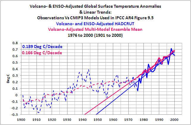
Figure 6
HHHHHHHHHHHHHHHHHHHHHHHHHHHHHHHHHHHHH

Figure 7
HHHHHHHHHHHHHHHHHHHHHHHHHHHHHHHHHHHHH
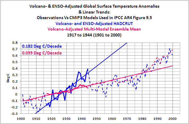
Figure 8
HHHHHHHHHHHHHHHHHHHHHHHHHHHHHHHHHHHHH
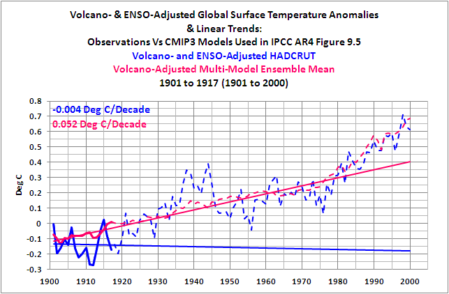
Figure 9
HHHHHHHHHHHHHHHHHHHHHHHHHHHHHHHHHHHHH
Adjusting the data for ENSO events and volcanic eruptions does not help to cure the ills of the climate models.
USING THE AVERAGE OF GISS, HADLEY CENTRE, AND NCDC GLOBAL SURFACE TEMPERATURE ANOMALY DATA
The IPCC chose to use HADCRUT3 Global Surface Temperature anomaly data for their comparison graph of observational data and model outputs in Chapter 9 of AR4. If we were to replace the HADCRUT3 data with the average of HADCRUT3, GISS Land-Ocean Temperature Index (LOTI) and NCDC Land+Ocean Temperature anomalies, would the model mean better agree with the observations? The trends of the late warming and mid-century “flat temperature” epochs still agree well, and trends of the early warming and early “flat temperature” periods still disagree, as illustrated in Figures 10 through 13.
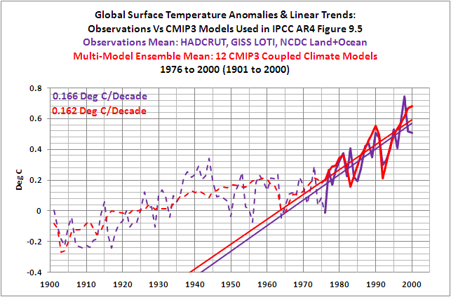
Figure 10
HHHHHHHHHHHHHHHHHHHHHHHHHHHHHHHHHHHHH

Figure 11
HHHHHHHHHHHHHHHHHHHHHHHHHHHHHHHHHHHHH

Figure 12
HHHHHHHHHHHHHHHHHHHHHHHHHHHHHHHHHHHHH

Figure 13
HHHHHHHHHHHHHHHHHHHHHHHHHHHHHHHHHHHHH
So the failure of the models is not dependent on the HADCRUT data.
SEA SURFACE TEMPERATURES – THE EARLY DIP AND REBOUND
When I first started to present Sea Surface Temperature anomaly data at my blog, I used the now obsolete ERSST.v2 data, which was available at that time through the NOAA NOMADS website. What I always found interesting was the significant dip from the 1870s to about 1910, Figure 14, and then the rebound from about 1910 to the early 1940s. Global Sea Surface Temperature Anomalies in the late 1800s were comparable to those during the mid 20thCentury “flat temperature” period.

Figure 14
NOTE: I wrote a post about that dip and reboundback in November 2008. The only reason I refer to it now is to call your attention to the first blogger to leave a comment on that thread. That’s John Cook of SkepticalScience. His explanations about the dip and rebound didn’t work then, and they don’t work now. But back to this post…
That dip and rebound exists to some extent in all current Sea Surface Temperature anomaly datasets, more so in the ERSST.v3b and HADSST2 datasets, and less so in the HADSST3, HADISST, and Kaplan datasets. Refer to Figure 15.

Figure 15
So how well do the model mean of the forcing-driven climate models compare with the long-term variations in Global Sea Surface Temperature anomalies? We’ll use the average of the long-term Sea Surface Temperature datasets that are available through the KNMI Climate Explorer, excluding the obsolete ERSST.v2. The datasets included are ERSST.v3b, HADISST, HADSST2, HADSST3, and Kaplan. And you will note in the graphs that the number of models has decreased from 12 to 11. TOS (Sea Surface Temperature) data for the MRI CGCM 2.3.2 was not available through the KNMI Climate Explorer. This reduces the ensemble members by 5 or about 10%, which should have little impact on these results, as you shall see. And you’ll also note that the years of the changeover from cooling to warming epochs and vice versa are different with the sea surface temperature data. The changeover years are 1910 (instead of 1917), 1944, and 1975 (instead of 1976).
As one would expect, the forced component of the models (the model mean) does a reasonable job of hindcasting the trend in sea surface temperatures during the late warming period, Figure 16, and also during the mid-century “flat temperature” period, Figure 17. The trend of the model mean during the early warming period, Figure 18, however, is only about 33% of the observed trend in the mean of the global surface temperature anomaly datasets. That failing is similar to the land-plus-sea surface temperature data. And then there’s the early cooling period, the dip of the dip and rebound, Figure 19. The model mean shows a slight warming during that period, while the observed Sea Surface Temperature anomaly mean has a significant negative trend. Yet another failing of the models.

Figure 16
HHHHHHHHHHHHHHHHHHHHHHHHHHHHHHHHHHHHH

Figure 17
HHHHHHHHHHHHHHHHHHHHHHHHHHHHHHHHHHHHH
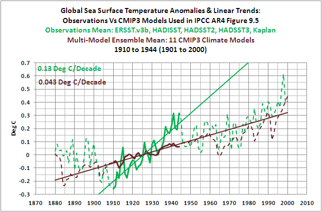
Figure 18
HHHHHHHHHHHHHHHHHHHHHHHHHHHHHHHHHHHHH

Figure 19
HHHHHHHHHHHHHHHHHHHHHHHHHHHHHHHHHHHHH
THE IMPACT OF THE 1945 DISCONTINUITY CORRECTION
If you were to scroll up to the Sea Surface Temperature dataset comparison, Figure 15, you’ll note how the HADSST3 data is the only Sea Surface Temperature anomaly dataset that has been corrected for the 1945 discontinuity, which was presented in the previously linked paper Thompson et al (2009). Raising the Sea Surface Temperature anomalies during the initial years of the mid-century flat temperature period has a significant impact on the observed linear trend for that epoch. And as one would expect, the trend of the model mean no longer comes close to agreeing with the HADSST3 data during the mid-century “flat temperature” period, because the observed temperature anomalies are no longer flat, as illustrated in Figure 20.

Figure 20
ENSO INDICES DO NOT REPRESENT THE PROCESS OF ENSO
Earlier in the post I noted that Thompson et al (2009) had assumed global temperatures respond proportionally to ENSO, and that that assumption was wrong. I have been illustrating that fact in numerous ways in dozens of posts over the past (almost) three years. The most recent discussions appeared in the following two-part series that I wrote at an introductory level:
ENSO Indices Do Not Represent The Process Of ENSO Or Its Impact On Global Temperature
AND:
DO OBSERVATIONS AND CLIMATE MODELS CONFIRM OR CONTRADICT THE HYPOTHESIS OF ANTHROPOGENIC GLOBAL WARMING?
Just in case you missed the obvious answer to the title question of this two-part post, the answer is they contradict the hypothesis of anthropogenic global warming. The climate models presented by the IPCC in AR4 show how global surface temperatures should have risen during the 20th Century if surface temperatures were driven by natural and by anthropogenic forcings. As illustrated in Figure 5, the climate models show that surface temperatures during the late 20th Century warming period, from 1976 to 2000, should have risen at a rate that was approximately 2.9 higher than the rate at which they warmed during the early warming period of 1917 to 1944. But, as shown in Figure 1, the observed rates at which global temperatures rose during the two warming periods of the 20thCentury were the same, at approximately 0.175 deg C/decade.
CLOSING
In this post we illustrated that…
1. regardless of whether we adjust global surface temperature data for ENSO and volcanic aerosols,
2. regardless of whether we use the global surface temperature dataset presented by the IPCC in AR4 (HADCRUT3) or use the average of the GISS, Hadley Centre, and NCDC datasets, and
3. regardless of whether we examine global land-plus-sea surface temperature data or only global sea surface temperature data
…the model mean (the forced component) of the coupled ocean-atmosphere climate models selected by the IPCC for presentation in their 4thAssessment Report CANNOT reproduce:
1. the rate at which global surface temperatures fell during the early 20thCentury “flat temperature” period, or
2. the rate at which global surface temperatures warmed during the early 20thCentury warming period.
The model mean (the forced component) of those same climate models CANNOT reproduce the rate at which global surface temperatures fell during the mid-20thCentury “flat temperature” period if the Sea Surface Temperature data during that period have been corrected for the “1945 discontinuity” discussed in the paper Thompson et al (2009).
As illustrated and discussed in parts 1 and 2 of this post, global surface temperatures can obviously warm and cool over multidecadal time periods at rates that are far different than the forced component of the climate models used by the IPCC. This indicates that those variations in global surface temperature, which can last for 2 or 3 decades, or longer, are not dependent on the forcings that were prepared solely to make the climate models operate. What then is the purpose of using those same models, based on assumed future forcings, to project climate decades and centuries out into the future? The forcings-driven climate models have shown no skill whatsoever at replicating the past, so why is it assumed they would be useful when projecting the future?
ABOUT: Bob Tisdale – Climate Observations
SOURCES
NOTE: The Royal Netherlands Meteorological Institute (KNMI) recent revised the security settings of their Climate Explorer website. You will likely have to log in or registerto use it. For basic information on the use of this valuable tool, refer to the post Very Basic Introduction To The KNMI Climate Explorer.
The sea surface temperature and combined land+sea surface temperature datasets are found at the Monthly observationswebpage of the KNMI Climate Explorer, and the model data is found at their Monthly CMIP3+ scenario runswebpage.
For the Global HADSST2 data, I used the data available through the UK Met Office website, specifically the annual global time-series data that is found at this webpage, then changed the base years for the anomalies to 1901-1950.
I’m confused by this statement also:
“…global surface temperatures are capable of varying without natural and anthropogenic forcings.”
If a forcing is not natural or anthropogenic, what other category could it fall under? Supernatural? What other possibilities are there?
Dr. Dan;
Try Wordpad. Much less demanding and more compatible.
If by definition there are forcings, they may be
a) individually weak
b) not included in the models
c) unknown.
Pick one, two or three of the above.
Smokey says:
December 12, 2011 at 7:31 pm
Gates, let an expert explain it for you:
For small changes in climate associated with tenths of a degree, there is no need for any external cause. The earth is never exactly in equilibrium. The motions of the massive oceans where heat is moved between deep layers and the surface provides variability on time scales from years to centuries. Recent work suggests that this variability is enough to account for all climate change since the 19th Century.
~Prof Richard Lindzen
Skeptics understand that climate is not like a roulette wheel. It’s the UN/IPCC that peddles that sort of nonsense.
———-
Smokey,
“The motions of massive oceans where heat is moved between deep layers…” is a completely deterministic process. And certainly is does provide variability as Lindzen so describes, and that creates a forcing on the climate. But it is a critical error to suggest that variability does not amount to a natural forcing as certainly it does. From Milankovitch cycles to solar variations lasting decades or centuries, greenhouse gas concentrations and volcanic activity, all these provide natural variability that is both deterministic and chaotic.
It is not just the honest skeptics who understand that the climate is not like a roulette wheel, but all climate scientists, who with each new discovery, fill in a bit more of the full deterministic interactions of this amazingly complex and beautiful climate system.
Philip Bradley says:
“And I’ll note you haven’t addressed my point that climate can be affected by factors that affect feedbacks. Unless you say all factors affecting feedbacks are automatically forcings. But then it starts to look tautological.”
———–
Please give some examples of what you consider to be “factors that affect feedbacks”. In my mind, the very laws of physics right down to the quantum level could be considered as a factor affecting feedbacks. For example, the absorption spectrum of both water vapor or CO2 is determined by the specific electron configuration of the molecules, and this is a factor that affects feedback. The distinction between a factor affecting a feedback and a forcing is one of form versus actual function. The factors are forms that determine function…i.e. The laws of physics are the form, and the actual variation in solar energy striking the earth or LW being absorbed by greenhouse gases are the functions.
Brian H says:
December 12, 2011 at 10:01 pm
If by definition there are forcings, they may be
a) individually weak
b) not included in the models
c) unknown.
Pick one, two or three of the above.
———-
Forcings may:
1) be weak or strong
2) be short-term, long-term, and everything in between
3) be included or not in the models and to greater or lessor degrees of accuracy
4) be known or unknown
5) be natural or anthropogenic
6) work in concert or in opposition to each other
7) produce their own unique set of feedbacks or unique combinations of feedbacks when multiple forcings are at work
Louis says:
“If a forcing is not natural or anthropogenic, what other category could it fall under? Supernatural? What other possibilities are there?”
He’s merely stating that global average temperature is subject to “drift” or variation without an external forcing, i.e.: internal variability. This part is not controversial (see Gavin quote above). The post demonstrates quite well that the climate modelers’ claim that “ensembles” of climate models cancel out similar internal variation revealing the projected global average temperature due to forcings and thus mimics the climate is not supported by historical observations.
Either the models are missing significant forcings, or, ensembles of models don’t cancel out internal variation analogous to the climate, or, the models don’t accurately approximate forcing vectors. The ensembles of models don’t accurately reflect the effect of forcings, feedbacks, and internal variability on global average temperature as evidenced by it’s inability to accurately hindcast the 1917-1944 0.175 deg C/decade warming, the 1944-1976 warming hiatus, AND the 1976-2000 0.175 deg C/decade warming. The fact that the ensemble matches one of these three periods is insufficient verification that it can be trusted to accurately project future climate trends as claimed.
Dishman says:
December 12, 2011 at 5:06 pm
R. Gates wrote:
Climate is not a random walk, nor does it exist in a state of quantum uncertainty.
This is true only if you define Climate as the ensemble of all random-walks, including weather and longer term variability. If that is your definition, then whether or not we actually know Earth’s current climate is at best in dispute.
——–
Of course I would not define climate an the ensemble of random walks, but rather the physical manifestation of the sum product of all actual forcings working through specific laws of physics to create, control, and otherwise manipulate the flow of energy to, from, and within Earth’s atmosphere, hydrosphere, and biosphere.
R.G.;
My list of 3 was not an exhaustive list of types/characteristics of forcings, merely a statement of what may render any claim to have such an exhaustive and well-characterized list dubious or non-functional. Particularly one composed of/headed by candidates selected by exclusion or argument from ignorance. Such as CO2.
Without getting into a long discussion about what is a feedback, I’ll define it as any net climate warming/cooling process that is not directly a radiative forcing.
An example of a feedback is heat transport upwards in the atmosphere by water vapor and then heat release thru condensation/precipitation. This process occurs primarily as a consequence of radiative heating of the surface.
Anything that affects the speed of this process will affect the speed of heat loss to space. Make it faster and the climate cools. Recent studies show a large effect by aerosols on water vapor condensation/precipitation. While the studies didn’t measure the time from surface evaporation to condensation/precipitation, its a reasonable inferrence that they accelerate the process. Thus acting to cool the climate by affecting a feedback.
R. Gates says: “You’ve not addressed at all the key issue I had with your summary from part 1…”
Thanks for the reminder. You began that comment with, “So, please give an example of global surface temperatures varying without some natural or anthropogenic forcing.”
When you read the term “internal variability” in a paper, don’t you interpret that to mean unforced?
I’m sure you’ve heard of the Atlantic Multidecadal Oscillation, which is principally expressed as natural multidecadal variations in the Sea Surface Temperature anomalies of the North Atlantic. It is considered to be one of the forms of internal, unforced climate (surface temperature and pressure) variability. One of the key papers to investigate the process was Knight et al (2005):
http://holocene.meteo.psu.edu/shared/articles/KnightetalGRL05.pdf
They isolated the internal variability by maintaining constant levels of external forcing. So it is believed the surface temperature of the North Atlantic can vary on a multidecadal basis without “some natural or anthropogenic forcing” causing those variations.
Bob,
if you have time to do so, could you please comment on this new approach here …
http://www.iac.ethz.ch/people/knuttir/papers/huber11natgeo.pdf
Roger Pielke sen. has left a comment over at his blog but it would be interesting to learn what you think about it.
Thanks
Ray Berger
Ray Berger says: “Bob,if you have time to do so, could you please comment on this new approach here …”
Huber and Knutti (2011) is a climate model study. Enough said.
It’s quite informative to look at what the adjustments made by hadSST3 look like.
Here is a plot of the difference between hadSST3 and the ICOADs data it is based on:
http://oi44.tinypic.com/1zee6ut.jpg
Note the vertical temperature scale here, The adjustments are almost a big as the whole of 20th warming we’re all supposed to sacrifice our futures to for. So do they make sense? Here’s some points worth noting:
The post war cooling discontinuity gets partially “corrected” when it occurred (which was from one month to the next) the rest gets faded it in a way that reduced the trough before 1960 as Bod noted. If you look at the difference between 1939 and 1946 there was still a huge 0.15C cooling over such a short period, that would be remarkable. In fact they only correct half the discontinuity.
The huge warming of the pre war period. What’s this about ?
Well from 1885 to 1920 there is a 0.3 warming “correction”. From then on to 1940 a 0.1 cooling. If we recall what Bob says about the inconvenient dip and rebound you can see they’ve fixed the model by changing the data.
Finally a little up tick after 2000 the “hide the decline”.
In fact looking at the general form of this adjustment it has what looks like a cyclic trend of about 140y that hit it’s trough around 1990. Did someone say “natural” cycles ?
Well there used to be one, but this adjustment just happens to be the other way up.
Now I’m not suggesting that Thompson et al and the rest of the Met Office are a bunch of crooks trying to deceive the world by removing any natural trends form the data and frig the data to fit their super computer models. But if they were , they may well be tempted to produce something very similar to the adjustments contained in hadSST3.
If anyone wanted to look for a natural cycle , I think the M.O. have done a great job of identifying for us.
Bob T. et. al.,
I appreciate the general perception by some that the fluctuation, or as some call “internal variability” of the AMO does not stem from some forcing, but this perception is by no means universal. I would direct your attention to just a few examples:
http://meetingorganizer.copernicus.org/EGU2009/EGU2009-4926.pdf
http://www.nature.com/ngeo/journal/v3/n10/full/ngeo955.html
http://www.sciencedirect.com/science/article/pii/S0273117707005418
When I hear the term “natural variability” or “internal variability” I immediately get the notion that “we really don’t know what is causing these fluctuations, so we’ll just call it ‘natural or internal variability’.
R. Gates: Your opinion is noted. That doesn’t mean I agree with it. I’ve read it. We’ve both shown that we can provide links to climate studies that support forced or unforced variability of North Atlantic Sea Surface Temperatures. That’s a no-win discussion. So let’s change tacks.
We’ll change roles. Now I’ll ask you a question. Let’s make it two. They’re easier to phrase as two sentences. There’s a long introduction, though.
In all of the early warming period (1917-1944) graphs above, surface temperatures are shown to be warming at rates that are around 3 times faster than the model mean data. And the rates at which surface temperatures rose in the early period are always comparable to the surface temperature trends in the late warming period (1976-2000). And based on the quotes from Gavin Schmidt and NCAR, we have interpreted the model mean to be the forced component of the climate models. And let’s assume for these questions that the observational data are correct and the forced components (model mean) are correct; the climate scientists have had 20plus years to get the forcings right, and the climate modelers have also had 20plus years to tune the climate models so that they respond properly to the forcings. You claim the difference between trends of the model mean and the trends of the observed rise in temperature during the early warming period cannot be caused by an unforced component, because unforced components don’t exist. How then do you explain (in plain English, for those without technical backgrounds who are reading this) the additional rate at which surface temperatures rose during that early warming period? And why are the rates at which surface temperatures rose during the early warming period (1917-1944) and the late warming period (1976-2000) comparable, while the forcings have risen by a factor of about three?
Interesting thread.
Thanks to Bob and others including R, Gates.
“The failure of the models to hindcast the early rise in global surface temperatures also illustrates that global surface temperatures are capable of varying without natural and anthropogenic forcings. ”
I vote for super-natural forcings.
In this situation (all forcings removed – except the super-natural ones) the Earth’s temperature *will* vary. The variations will be on a steadily decreasing trendline; it will grow cold. All of its internal heat will fade away and radiate into space.
This has nothing to do with the failure of models, it’s gobbledy-gook purdeed up with graphs.
Bob T. asked:
Question 1: “How then do you explain (in plain English, for those without technical backgrounds who are reading this) the additional rate at which surface temperatures rose during that early warming period?”
Question 2: “And why are the rates at which surface temperatures rose during the early warming period (1917-1944) and the late warming period (1976-2000) comparable, while the forcings have risen by a factor of about three?”
_____
As a background to answer both these questions, let me just take a brief detour for a moment to go back to my fundamental position, and that is that all climate change is related to a forcing or more common, a combination of forcings. So called “natural variability” or “internal variability” is simply a chaotic system of forcings that haven’t been (or can’t be, based on our current mathematics) put into a model. The very fact that there is a periodicity to the AMO, for example, is a wonderful example of a chaotic oscillating system. This is a system that is deterministic, not random, and thus some forcing or combination thereof drives it, we simply haven’t the tools to fully model it.
Now, to answer your questions in plain English. Not all models do as poor a job at hindcasting the rapid rise in temperatures during the period of 1917-1944, nor of course, the end of the 20th century during the period of 1976 – 2000. I would highly advise you and others read this full research article:
http://onlinelibrary.wiley.com/doi/10.1002/wcc.18/full#fig2
In simple terms, some (but not all) models failed in their ability to model the early 20th century warming, as the totality of solar forcing influences, including EUV affects on ozone and stratospheric circulation (which have only recently been quantified and added to some models), were underestimated, and when included, match up well with the early 20th century temperature rise. See:
http://scostep.apps01.yorku.ca/wp-content/uploads/2010/07/Gray_etal_2009RG000282.pdf
This answers question 1. Which is– the models which take into account to full range of solar forcing do a good job at displaying the early 20th century temperature increases.
For question 2, your assumption seems to be that the same apparent effect (i.e. a temperature rise) has the same combination of forcings as its cause, and though the temperature rise in the early 20th century might appear to be the same as the later 20th, the models would actually disagree with you, and even very nicely break down the different types of forcings (natural and anthropogenic) that caused each period of temperature increases. So to say that the “forcings have risen by a factor of 3” is an incorrect statement. Some forcings decreased while some forcings increased. What matters to make up the climate is of course the net result of all forcings combined. Furthermore, the early 20th century temperature rise (as measured by troposphere temps or ocean temps, was not identical to the late 20th century temperature rise, in that stratospheric temperatures were rising in the early 20th century, but were falling in the later 20th century. Thus, the early 20th century temperature rise has a more classic solar influence signature and of course, the later 20th century, would be more indicative of greenhouse gas forcing. A perfect example of the combination of forcings leading to a net result that is not as simple as saying “a tripling of forcings” is the flattening of temperatures during the last decade, during which time the decreased activity of the sun, increased volcanic activity and human aerosol creation have pretty much masked the visible greenhouse gas forcing for the time being. I would love to see a model run with the current low solar output combined with the additional aerosols and the extended La Nina period but with CO2, N2O, and methane kept at pre-industrial levels. It will be interesting to see which prevails in the short-term, though in the long-term, the continually rising greenhouse gases certainly will.
Thus, the early 20th century temperature rise has a more classic solar influence signature and of course, the later 20th century, would be more indicative of greenhouse gas forcing.
There is evidence to support this position. For example the paper below. Which shows solar effects have a better correlation with 20th century temperatures up until 1990
http://adsabs.harvard.edu/abs/2008AGUSMGC43A..06M
But then we run into the CO2 lag problem that CO2 rises lag temperature rises since 1970. Causation can never work backwards.
http://www.nature.com/nature/journal/v343/n6260/abs/343709a0.html
Its a pet issue of mine that determining what causes (say annual) changes in the climate is a fairly easy statistical exercise assuming you have decent measurements. Climate science avoids these analyses like the plague because they show CO2 changes have close to zero correlation with annual temperature changes.
http://www.scirp.org/Journal/PaperInformation.aspx?paperID=3447&utm_source=newsletter&utm_medium=ijg13&utm_campaign=01
What they resort to (as R Gates does) is a priori arguments. Which is OK as long as your underlying theory is sound. If it isn’t, a priori arguments are worthless.
So we come down to our point of difference, is the Forcing model a valid theory of climate change?
I think the data indicates it doesn’t have sufficient explanatory/predictive power to be a valid theory of climate change, and Bob’s analysis adds to this evidence.
No amount of a priori argument will persuade me. Only data will.
Finally, it is a perfectly valid scientific answer to say ‘we don’t know what causes climate change’.
R. Gates says: “Not all models do as poor a job at hindcasting the rapid rise in temperatures during the period of 1917-1944, nor of course, the end of the 20th century during the period of 1976 – 2000. I would highly advise you and others read this full research article: http://onlinelibrary.wiley.com/doi/10.1002/wcc.18/full#fig2”
The period in question is not the late warming period of 1976-2000. As illustrated in this post, the models have problems with the early warming period of 1917-1944. If you were to look at Figure 6 of Lean 2010 you’d note Judith Lean’s empirical model actually does a very poor job of recreating the rise in surface temperature from 1917 to 1944. It’s comparable to the poor job of the model mean of the IPCC’s models from Figure 9.5 of AR4. And I believe our discussion pertains to the general circulation models used in AR4 for their hindcast comparison. Please advise the readers who are following this thread what coupled ocean-atmosphere model was presented by the Lean 2010 paper that you linked. I’ll save you some time. There wasn’t one. The empirical model (based on linear regression analysis) was presented in the Lean and Rind (2009) paper “How will Earth’s surface temperature change in future decades?”
http://www.unity.edu/facultypages/womersley/2009_Lean_Rind-5.pdf
R.Gates says: “In simple terms, some (but not all) models failed in their ability to model the early 20th century warming…”
In reality, the model mean for all the CMIP3 models chosen by the IPCC for their Figure 9.5 model-observations comparison (and reproduced as Figure 27 in your linked Gray et al 2009) “failed in their ability to model the early 20th century warming”:
http://i40.tinypic.com/11ueu7p.jpg
I produced Table 1 for part 1 of this post, but I decided it would detract from the post, so I didn’t include it.
R.Gates says: “This answers question 1. Which is– the models which take into account to full range of solar forcing do a good job at displaying the early 20th century temperature increases.”
The model data (Table 1) disagrees with your assumption, because no models “do a good job at displaying the early 20th century temperature increases”.
R. Gates says: “For question 2, your assumption seems to be that the same apparent effect (i.e. a temperature rise) has the same combination of forcings as its cause………..”
I’ll re-ask the second question. I accidentally wrote “forcings” instead of “forced component of the models.” My mistake. The forcings had risen by a factor of four. It was the forced component (the model mean) that rose by a factor of three. Sorry. Here’s the question again:
And why are the rates at which surface temperatures rose during the early warming period (1917-1944) and the late warming period (1976-2000) comparable, while the forced component (the model mean) have risen by a factor of about three?
Posted on December 12, 2011 by Anthony Watts
Do Observations and Climate Models Confirm Or Contradict The Hypothesis of Anthropogenic Global Warming?
Guest Post by Bob Tisdale
“Climate Models, on the other hand, do not recreate the rate at which global surface temperatures rose during the early warming period. They do well during the late 20thCentury warming period, but not the early one. Why? Because Climate Models use what are called forcings as inputs in order to recreate (hindcast) the global surface temperatures during the 20th Century. The climate models attempt to simulate many climate-related processes, as they are programmed, in response to those forcings, and one of the outputs is global surface temperature. …. The forcings-driven climate models have shown no skill whatsoever at replicating the past, so why is it assumed they would be useful when projecting the future?
I think the data available have to explained by physical processes and logic; a model that includes not the physics nor the well known relations and laws of nature cannot put out more than what is still known or unknown.
It would be great to simulate the hole dynamic solar system as perpetual motion using the physics of thermodynamic, heat currents and heat sources, and if this do not match with the size of a computer, we have to make it by Excel or by hand.
An example may be the nature of the sea level profiles in time. The University of Colorado has puplished a graph of the global mean sea level with a linear fit of the rising level of about 3.2 mm per year since 1993.
Beside some anomalies visible after a 60 day smooth a dropping of the sealevel of 6 mm in the year 2010 was discussed in the science community. But a detailed view on the oscillations before the 60 day smooth shows that the frequency of the mean oscillation superimposed to the linear increasing sea level is about 117 maxima in 18.655 years or 6.271 periods per year.
This is remarkable, because the synodic frequency of the planet couple of Mercury/Earth of 3.1519 periods per year [sf_me_er = 4.15194 – 0.99996 = 3.1519 y^-1] is exactly the half of the sealevel oscillation frequency from Jason-2 data of 6.271 periods per year.
It seems that there is no cause visible for a longtime linear sealevel rise of 3.2 mm per year, but I think it makes sense to analyse the mysterious superimposed frequency of twice the synodic Mercury/Earth frequency for several reasons.
The tidal effect on the Sun from the different bodies are, if Earth = 1.0: Jupiter = 2.26, Venus 2.15, Mercury at perihelion = 1.9, and Mercury at aphelion = 0.54. This means that the tide effects from the couple of Mercury/Earth on the Sun are varying depending on the distance of Mercury from its eccentric path.
The question comes up, why the measured global sealevel do rise and fall synchronous with the tide system of Sun, Mercury and Earth. But moreover, the oscillations of the global temperature measured from UAH fits in this tide profile:
http://volker-doormann.org/images/sealevel_vs_abc.gif
In the strong period of the sealevel height variation of 6.271 periods per year are several phase jumps, and amplitude variations which suggest one or more similar frequencies as the synodic tide frequency of Mercury/Earth. And adding three more synodic pattern from the couples of Venus/Earth, Mercury/Jupiter, and Earth/Jupiter because of their expected high tide effects the blue line results as a sum of the solar tide effects corresponding in geometry with the sea level oscillations.
This shows that here is a connection between the solar tide effects and the global temperatures on Earth, along with a time coherent global sea level swing of some mm.
A rough calculation shows that a temperature change of 0.1°Cel of 1000 m deep ocean part results in a height change of ~23 mm because from the property of water. Whatever is the cause of this sea level dynamic of the substracted 3.2 mm per year function, solar tide effects of some planets play a role in this up and downs of as well sea level and SST. There are hints that other solar tide like couples beyond Jupiter can take a long term increase of the global temperature, which could explain the seeming ‘linear’ ocean height rise of 3.2 mm per year in the last 18 years.
However, it will take good ideas from physics to explain the shown connection between solar tide geometries, the sea level change and terrestrial climate frequencies as a heat current from the Sun.
I think this method is superior to simple models feed with functions of no base in real nature, especially because it has the capability to simulate climate of the history and of the future in high fidelity.
Science has not to show what is not. Science has to show what IS.
V.
Is what’s good for the goose not good for the gander?
On RC Rasmus Benestad discredits the predictive value of a statistical model presented in a recent paper by hindcasting and demonstrating the hindcast does not match the proxy derived temperature tends.
“It is well known that one can fit a series of observations to arbitrary accuracy without having any predictability at all. One technique to demonstrate credibility is by assessing how well the statistical model does on data that was not used in the calibration.” http://www.realclimate.org/index.php/archives/2011/12/curve-fitting-and-natural-cycles-the-best-part/#bib_1
Bob Tisdale has discredited the predictive value of the AR4 models as well as the ensemble with the same technique, yet this is somehow inappropriate here (WUWT) on “physical” models but is appropriate at RC on “statistical” models. [see above]
Are we to believe that because of their authority on the subject that even though their models don’t hindcast well that they still have predictive value even though they dispute the predictive value of another’s model because it doesn’t hindcast well?
Why shouldn’t physical models be able to demonstrate predictive value in the same way as statistical model is expected to be able to?
Why should “experts” get a pass on the test that they use to criticize “amateurs”?
We’ve recently seen evidence that even models that hindcast well may not have predictive value. That internal variation is inherently unpredictable and its magnitude overwhelms the conjectured anthropogenic forcing.
http://wattsupwiththat.com/2011/12/13/csus-klotzbach-and-gray-suspend-december-hurricane-forecast/
Why should models that don’t hindcast well be considered predicatively skillful?
As it has been said many times in many ways by many people on WUWT: How many years and how many ways must the models diverge from observations before they are rejected as useless video game novelties?
John West says: “Bob Tisdale has discredited the predictive value of the AR4 models as well as the ensemble with the same technique, yet this is somehow inappropriate here (WUWT) on ‘physical’ models but is appropriate at RC on ‘statistical’ models.”
Who said my analysis was inappropriate?