Guest post by Steve Goddard
UPDATE 1-15-08:
I tried an experiment which some of the null questioners may find convincing. I took all of the monthly data from 1978 to 1997, removed the volcanic affected periods, and calculated the mean. Interestingly, the mean anomaly was positive (0.03) i.e. above the mean anomaly for the 30 year period.
This provides more evidence that normalizing to null is conservative. Had I normalized to 0.03, the slope would have been reduced further.
Yesterday’s discussion raised a few questions, which I will address today.
We are all personally familiar with the idea that reduced atmospheric transparency reduces surface temperatures. On a hot summer day, a cloud passing overhead can make a marked and immediate difference in the temperature at the ground. A cloudy day can be tens of degrees cooler than a sunny day, because there is less SW radiation reaching the surface, due to lower atmospheric transparency.
Similarly, an event which puts lots of dust in the upper atmosphere can also reduce the amount of SW radiation making it to the surface. It is believed that a large meteor which struck the earth at the end of the Cretaceous, put huge amounts of dust and smoke in the upper atmosphere that kept the earth very cold for several years, leading to the extinction of the dinosaurs. Carl Sagan made popular the idea of “nuclear winter” where the fires and dust from nuclear war would cause winter temperatures to persist for several years.
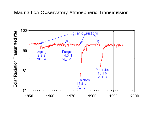
Large volcanic eruptions can have a similar effects. This was observed in 1981 and 1992, when volcanic eruptions caused large drops in the measured atmospheric transmission of shortwave radiation at the Mauna Loa observatory. These eruptions lowered atmospheric transmission for several years, undoubtedly causing a significant cooling effect at the surface. At one point in late 1991, atmospheric transmission was reduced by 15%. An extended period like that would lead to catastrophically cold conditions on earth.
In recent years, there has been a lot of interest in measuring how much warming of the earth has occurred due to increased CO2 concentrations from burning fossil fuels. This is difficult to measure, but one thing we can do to improve the measurements is to filter out events which are known to be unrelated to man’s activities. Volcanoes are clearly in that category. In yesterday’s analysis, I chose to null out the years where atmospheric transparency was affected by volcanic eruptions, as seen in the image below. Atmospheric transmission is in green, and UAH satellite temperatures are in blue.
Atmospheric transmission in green. Monthly temperature deviation in blue, with overlap periods nulled out.
The question was raised, why did I null out those periods?
I made that decision because the null level is the mean deviation for the period, and because that is the most conservative approach. As you can see in the image below, there is a large standard deviation and variance from month to month, which makes other approaches extremely problematic. There were also corresponding El Ninos during both of the null periods, which would have been expected to raise the temperature significantly in the absence of the the volcanic dust. Had I attempted to adjust for the El Nino events, the reduction in slope (degrees per century) would have been greater than what I reported. This is because the temperature anomaly during each El Nino would have been greater than zero (above the null line.)
Due to the large standard deviation and large monthly variance, any attempt to calculate what the temperature “should have been” in the absence of the volcanic dust would likely introduce unsupportable error into the calculation. One can play all sorts of games based on their belief system about what the temperature should have been. I chose not to do that, and instead used the mean as the most conservative approach.
There is no question that the volcanic dust lowered temperatures during those periods, and because of that the 1.3C/century number is too high. My approach came up with 1.0. A reasonable ENSO based approach would have come up with a number much less than that. If you take nothing else away from this discussion, that is the important point.
UAH, with non-nulled temperatures in green.
Furthermore, it is also important to realize that the standard approach of reporting temperature trends as linear slopes is flawed. Climate is not linear, which is why Dr. Roy Spencer fits his UAH curves with a fourth or fifth order function, rather than a line.
I’ve been thinking (always a dangerous thing!) about this…
The best thing to do seems to depend on what duration of trend you want to find and the relative sizes of ‘gap’ and oscillations in the data. If you are looking for the trend over the entire range of data (long term warming signal), I would concatenate the data minus the gaps, then fit a least squares line through it, find the slope of that line, and then use that slope for ‘infill’ data. This would be my base case.
I could see using that base case to do another fit and get an even more representative slope for the infill (iteration #2) but doubt if the change would be significant.
For shorter duration trends of interest you would need to use shorter spans of data for the LSF to create infill more representative of local conditions. At some limit short range you begin to create too much error by amplifying local oscillations where you have partial cycles in the data being least square fit… such as the ‘ramp’ leading into gap #2.
In particular, and of relevance here, only the particulates in the stratosphere will have enough dwell time to affect weather. Turbulence of the tropopause and the physical size of the particulate determine dwell time. (Particulates below the tropopause settle out within hours.)
The maximum dwell for particulates above the tropopause is a few years. Particulates on the order of 100 microns settle out within a few days, on the order of 10 microns within a few weeks, and so on. All particulates will have settled out within 24 to 36 months.
Very interesting.
Question (for all): What of the effect of aerosols that do make it to the stratosphere? Would they not come out primarily at the poles and 30 N and S?
They would obviously have a much lower albedo than polar ice so they would also have a positive contribution to total solar insolation absorbed by the surface over the course of, potentially, 24 – 36 months!?! I wonder if the net effect 2 years after a major eruption has been thoroughly fleshed out…
Steve Goddard
Using relaxation, the slope for the UAH in the woodfortrees data you listed in your post to Filipe, is 0.009067 plus/minus 0.0032% difference for removing the data indicated in your part 1 using linest in Excel and relaxation as I posted. As I also indicated, it improves your argument. The trend is lower, plus you replace the data, not with null data, but with the estimate of the trend, such that claims of incorrectly weighting are answered by the assumption. The assumption is that there is a linear trend, that volcanoes (plus or minus) are not part of. By replacing the data with the trend of the remaining data, your corrected slope is as neutral as possible.
For this period, assuming no net forcing for volcanoes, the predicted increase in temperature based on the average rate of the period used for the estimation will be 0.907 C degrees per century.
John Pittman,
Thank you very much for your explanation and calculations. That is what WUWT is all about!
Katherine says:
Sorry about that. I did realize that I had made that mistake and issued a post correcting it (time stamp 07:58:38, 15/1/09) which ended up 3 posts down from my original post.
Well, I should have checked my work twice. I got your number Steve. The corrected is 0.0118 +/- 0.06% difference.
Ok, I just did it using robust ** methods. The slope goes from 1.3 K/century with the full data to 1.0 K/century by removing the period with the volcanoes (I prefer Kelvin since it spares me the degrees). It’s almost the same result as the regular least squares, confirming that Steve’s result isn’t controlled by a possibly well placed outlier.
That’s not totally unexpected since the monthly residuals follow a nearly gaussian distribution with standard deviation 0.16 K (+-.01K). In these conditions least squares should perform rather nicely. One can even put an error bar in the slope from least squares. The error in the estimated slope is about 0.12 K/century, So we have an 8-sigma “warming” signal at 1.0 K/century.
** least squares «reacts badly» when replacing even a single point by a very large outlier (it has a rupture limit of zero). Methods which use the median of all possible pairs of points like Theil and Sen allow something like 29% of random outliers, while the repeat median from siegel can tolerate something like 50% random outliers. I checked both.
I would like to note also that this is just a way to infer if the data follow an increasing or decreasing behaviour in THIS time interval, and if it mimics the trend expected from models.
Filipe,
Thanks for following up!
It appears that the statistical experts here came up with a slope as low or lower than my original analysis, confirming that my calculation was conservative. Given the coincident El Nino events, a climatologically corrected adjustment would likely have produced slopes less than 1.0K/century.
It is interesting, but not expected, that the three different methods give essientially the same number. I also get 1.175K/century by replacing the highest 1998, and the lowest 2008 with the estimated slope indicating that the the estimated signal remains with removal of the “battle of the weather noise” complaints. You can play around with outliers, decrease and increase the spliced parts, but they all hang around that 1.1 to 1.2 K/century, providing futher confirmation that using the satellite data without accounting for “cooling the past” by the random effect of volcanoes will give a higher predicted trend. It also confirms why people have expressed their concern about GISS cooling the past. Such methodology DOES give a higher trend, real or not.
The potential for problems is shown by a mathematical example, below. So I took my corrected UAH data for volcanoes and the 1998/2008 “”weather”” and computed a trend of 1.14 K/century, the lowest I got without cherry picking. The next step was to go to the midpoint and compute the average, which is 0.097668439. Next, I computed each point forward and backward from the midpoint where I inserted the average, replacing the actual data with the computed data generated by our slope of 1.14 K/century. So what happens if you correct for 1 K in one century on a monthly basis? With this assumption 1K/100 years/12 months equals 0.000833333. Then from the midpoint backwards to the start, I subtracted stepwise 0.0008333 each month to induce a “cooling of the past”; and I added 0.0008333 each month to induce a systemic rise such as unaccounted UHI effect in a stepwise manner, or GISS “correction”. Then I computed, using LINEST in Excel, the trend. The trend went from 1.144 k/Century to 2.144 K/century. Not really unexpected is it? A cooling of 1K per century from the present to the past, induces an addition of 1K per century to the trend.
Now, exactly what does GISS, Hadley, and others do? It is quite easy to prove that it matters; as would the local anthropogenic effect of introducing warming in the recent decades. So lets correct using a step change for a step change. Replace the 1.144 trend endpoints with the 2.144 trend endpoints and compute the LINEST, it is now 1.161, not 2.144. So using a trend to replace a stepfunction introduces a false trend in a computation. As has been pointed out several posters, whether you do this at the beginning or end, or both, can impart a false trend in your computations.
The question is “What does the homogenization by GISS impart to the trend, if a step function occurs and the data is changed incrementally rather than as a step change”.
John Pittman,
I always expected that everyone would come up with approximately the same number. My reasoning being that the unaffected period from 1978-1997 was essentially a flat line, masked by a Gaussian scatter. Any correct method of analysis involving substitution or elimination would thus come up with essentially the same answer.
“My reasoning being that the unaffected period from 1978-1997 was essentially a flat line, masked by a Gaussian scatter”
Yes, if you order the residuals and compute the 16% and 84% percentil you get a robust estimator for twice the standard deviation. When you then bin the residuals and compare the histogram with the gaussian for that std the agreement in shape is rather remarkable.
On the other hand, when I do a fft to the data I do get a nice peak in my 8th shortest baseline (using the 361 months), so there is possibly one significant periodicity in the data.
The loudest volcano in recorded history , Krakatoa exploded Aug 26-7, 1883.
It is said that global temperature dropped by an average of 1.2 degrees C and that weather patterns were disrupted for five years.
In light of this, how ethical is it for Giss to start their global warming thermometer in the 1880’s?
And what of the pre 1880 record which must exist, since thermometers were invented in the 1400’s, and the historical record mentions a pre 1880 average temp?
http://home.casema.nl/errenwijlens/co2/ At Hans site you can get some nice graphs, and I believe access to the data underneath that answers your question papertiger.