How did the El Chichón and Pinatubo volcanic eruptions affect global temperature records? – Part 2

Guest post by Steve Goddard
UPDATE 1-15-08:
I tried an experiment which some of the null questioners may find convincing. I took all of the monthly data from 1978 to 1997, removed the volcanic affected periods, and calculated the mean. Interestingly, the mean anomaly was positive (0.03) i.e. above the mean anomaly for the 30 year  period.

This provides more evidence that normalizing to null is conservative. Had I normalized to 0.03, the slope would have been reduced further.

Yesterday’s discussion raised a few questions, which I will address today.
We are all personally familiar with the idea that reduced atmospheric transparency reduces surface temperatures.  On a hot summer day, a cloud passing overhead can make a marked and immediate difference in the temperature at the ground.  A cloudy day can be tens of degrees cooler than a sunny day, because there is less SW radiation reaching the surface, due to lower atmospheric transparency.
Similarly, an event which puts lots of dust in the upper atmosphere can also reduce the amount of SW radiation making it to the surface.  It is believed that a large meteor which struck the earth at the end of the Cretaceous, put huge amounts of dust and smoke in the upper atmosphere that kept the earth very cold for several years, leading to the extinction of the dinosaurs.  Carl Sagan made popular the idea of “nuclear winter” where the fires and dust from nuclear war would cause winter temperatures to persist for several years.
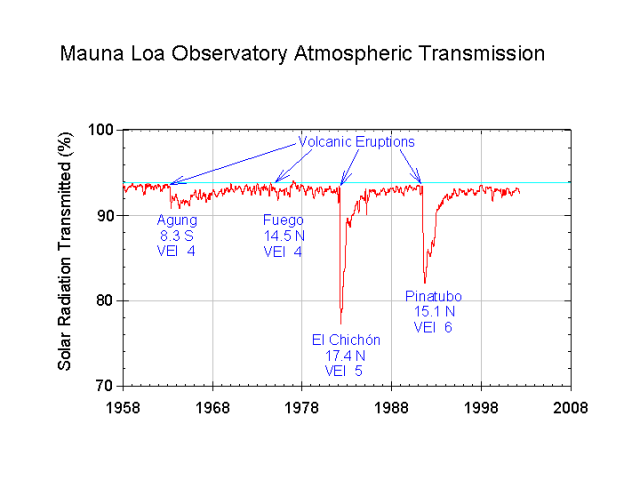
Large volcanic eruptions can have a similar effects.  This was observed in 1981 and 1992, when volcanic eruptions caused large drops in the measured atmospheric transmission of shortwave radiation at the Mauna Loa observatory.  These eruptions lowered atmospheric transmission for several years, undoubtedly causing a significant cooling effect at the surface.  At one point in late 1991, atmospheric transmission was reduced by 15%.  An extended period like that would lead to catastrophically cold conditions on earth.
In recent years, there has been a lot of interest in measuring how much warming of the earth has occurred due to increased CO2 concentrations from burning fossil fuels.  This is difficult to measure, but one thing we can do to improve the measurements is to filter out events which are known to be unrelated to man’s activities.  Volcanoes are clearly in that category.  In yesterday’s analysis, I chose to null out the years where atmospheric transparency was affected by volcanic eruptions, as seen in the image below.  Atmospheric transmission is in green, and UAH satellite temperatures are in blue.
Atmospheric transmission in green. Monthly temperature deviation in blue, with overlap periods nulled out.
The question was raised, why did I null out those periods?  
I made that decision because the null level is the mean deviation for the period, and because that is the most conservative approach.  As you can see in the image below, there is a large standard deviation and variance from month to month, which makes other approaches extremely problematic.  There were also corresponding El Ninos during both of the null periods, which would have been expected to raise the temperature significantly in the absence of the the volcanic dust.  Had I attempted to adjust for the El Nino events, the reduction in slope (degrees per century) would have been greater than what I reported. This is because the temperature anomaly during each El Nino would have been greater than zero (above the null line.)
Due to the large standard deviation and large monthly variance, any attempt to calculate what the temperature “should have been” in the absence of the volcanic dust would likely introduce unsupportable error into the calculation.  One can play all sorts of games based on their belief system about what the temperature should have been.  I chose not to do that, and instead used the mean as the most conservative approach.
There is no question that the volcanic dust lowered temperatures during those periods, and because of that the 1.3C/century number is too high.  My approach came up with 1.0.  A reasonable ENSO based approach would have come up with a number much less than that. If you take nothing else away from this discussion, that is the important point.
UAH, with non-nulled temperatures in green.
Furthermore, it is also important to realize that the standard approach of reporting temperature trends as linear slopes is flawed.  Climate is not linear, which is why Dr. Roy Spencer fits his UAH curves with a fourth or fifth order function, rather than a line.
0 0 votes
Article Rating
88 Comments
Oldest
Newest Most Voted
Inline Feedbacks
View all comments
January 15, 2009 12:42 am

I’m really starting to think that the temp trends are much flatter than advertised, something I wouldn’t have imagined even a year ago.
What adds to the conclusion of this post is the discontinuity in RSS from my last post. If you look only at the trend of the sat records, removing the discontinuity the average for RSS and UAH is only about 0.011 C/year for the LT. This should be 1.2 times the ground data.
Dr. John Christy UAH read my last article and provided an additional paper from 07 which confirms this discontinuity is the primary point of disagreement between RSS and UAH. What’s more the disagreement is resolved by checking radiosonde data leaving UAH as the superior measure.
After review of the data and the effects of the discontinuity, it is pretty obvous to me now that the flatter UAH trend is at this point more correct. Just cutting out the section of disagreement and averaging the remaining slopes puts the LTroposphere satellite slope at only 0.011 C/year which is very close to UAH 30 year trend of 0.127 C/decade.
http://noconsensus.wordpress.com/2009/01/15/1853/

Brooklyn Red Leg
January 15, 2009 12:54 am

Just to quibble for a moment, but wasn’t Nuclear Winter disproven because Sagan et al had calculated it based on force exchange that resulted in nothing but ground bursts (which produce LOTS of particulates/fallout) using weapons in the mutli-megaton range? This despite the fact that only hardened military targets (bunkers etc) would be ground-burst targets as well as the doctrine shift to smaller blast yields (standard Soviet and American was somewhere in the range of 550kT IIRC) using more efficient targeting vehicles due to improved technology. The days of the Tsar Bomba were long over.

Willem de Rode
January 15, 2009 12:59 am

I still wondering about the logics behind the reasoning.
If you leave out a natural cooling effect from a series of temperatures that shows a upward trend, then I think you must end up with a faster increasing trend !
It sounds complete unlogical to me that our planet warms up slower when one could take away the natural cooling events ?
Although the mathematics in these articles do give the reported results, these results appear to me contradictionary to the common sense that skipping a cooling fase must lead to a faster warming.
Sorry, but I think applying the reported mathematics on a series of global temperatures is scientific not justifiable or defendable.

John Finn
January 15, 2009 2:38 am

Steve Goddard
I’m not sure if you can answer this question, but what is the possibility to accurately model the volcano-affected years. I would have thought this would be relatively straightforward since NASA claim to have successfully modeled the Pinatubo cooling. In fact, the Pinatubo event is often used to justify GCM predictive skills.
The only other issue would be the ENSO effects which were positive either during or immediately after both eruptions. During 1982/83 there was a particularly intense El Nino, while ther were moderate El Ninos in 1991/92 and 1993.
In both cases, the affected periods would, without the volcanos, have likely included local temperature maximums, and, apart from the 1998 spike would leave the long term plot looking virtually flat.

John J
January 15, 2009 3:10 am

Steve
Something else this analysis points out is that there is a better way to control global warming. If man-made global warming exists, and I emphasize IF, and it is deemed a serious problem by a true consensus of rational experts, then the way to correct the problem may be to effect the albedo of the earth rather than totally rearrange the world’s economies. Whereas the idea of injecting SO2 into the upper atmosphere may sound ridiculous, when placed alongside the current plan of spending trillions of dollars on a solution that is not really a solution, it sounds extremely logical.

kim
January 15, 2009 3:33 am

‘Albedo’ is a word which eventually all citizens must come to understand. It is a fudge factor that will allow almost any interpretation to be placed on climate processes. It is fortunate that we have such things as discrete vulcanism to provide something on the order of a controlled experiment.
===========================================

January 15, 2009 3:33 am

Steve, your nulled out periods are still way too long. They need to be 1 and 2 yrs as per your Wiki chart.

Katherine
January 15, 2009 3:50 am

Willem de Rode wrote:
I still wondering about the logics behind the reasoning.
If you leave out a natural cooling effect from a series of temperatures that shows a upward trend, then I think you must end up with a faster increasing trend !
It sounds complete unlogical to me that our planet warms up slower when one could take away the natural cooling events ?

If you remove the natural cooling in the past, then the remaining signal is warmer. To give a numerical example, if the natural cooling resulted in an anomaly of -5 of the “normal” in the past and the present temperature anomaly is +5 (for a spread of 10), removing the natural cooling signal results in 0 anomaly (i.e., “normal”) in the past and therefore a spread of only 5, instead of 10.

January 15, 2009 4:11 am

Willem de Rode (00:59:26) :
“It sounds complete unlogical to me that our planet warms up slower when one could take away the natural cooling events ?”
Willem, it is the effect of WHERE in the timeline the cooling events have been zeroed out. Since both eruptions take place early in the time line, the zeroing out has effect of “warming up the past”. Thus, the overall observed warming trend flattens out – it’s still ending up in the same place, but the starting point is now higher than it was.
Personally, I think this a perfectly valid exercise. If Steve had decided to give the zeroed out periods a value higher than zero (as other have pointed out, the eruptions would have been “masked” an underlying warming trend) then the result would be a further flattening of the observed warming trend, making it approach zero, which is closer to the truth.
John J (03:10:17) :
It is my firm belief, bolstered by many of the things I have read on this subject over the years, that there is nothing to fix. I cringe every time I read of some grand plan to fix global warming (which I contend is entirely a social delusion, and not a fact of science) such as dumping scrap iron in the ocean to help algae fix more CO2, or to put aerosols into the atmosphere to reduce shortwave radiation from the Sun, or spraying water (a powerful GHG) into the air to cool it. Fixing a problem that does not exist is a recipe for disaster. None of these schemes have been thought through enough. Like the attempts to fix wildlife “problems” by controlling one species to favour another, we prove time and again that we are not capable of grasping the balance of nature, and create problems worse than the ones we thought we were solving (see Yellowstone, Australia, or Macquarie Island).
Honestly, we live on an ice planet that has occasional and brief periods of warmth. It is a bistable chaotic system that is in a cold phase for longer periods of time than in a warm phase, and we have people worrying it is “too warm”. I say, enjoy it while it lasts, because it won’t last forever. If anything is sure, we WILL experience another ice age (probably not within our lifetimes), as sure as the sun rises each morning.

Wally
January 15, 2009 4:39 am

The better approach is to just leave the data out for the volcano years not make it zero. Making them zero will artificially lower the absolute magnitude of the slope as well as decrease the standard deviation of the data. A plot of the slopes versus the number of months/years dropped from the data may be interesting.

Tom in chilled Florida
January 15, 2009 4:41 am

Willem de Rode ,
If we eliminate the effects of these two eruptions our starting point for temperature change is raised. This then reflects a lower rate of change to get to the temperatures we show today. If we accept this lower rate of change as real, then the AGW alarmists are wrong and we are not effecting the natural climate change as fast as they say we are.
What I don’t understand is why the AGW alarmists like to point out the so called “masking” of global warming by these eruptions. If that is correct and Steve is right then my first paragraph holds true and they fall on their own sword. Of course they do argue that using the lower temperatures created by the eruptions incorrectly lowers the average temperature for the chosen period. But I think they are mixing apples and oranges as one point addresses rate of temperature change over the period and the other addresses the average temperature over the period.
So, is the peanut gallery learning or do I need to sit quietly with muted fingers?

Pearland Aggie
January 15, 2009 4:48 am

while on the topic of temperatures…
All In
http://sciencepolicy.colorado.edu/prometheus/all-in-4873
It is a bit early in the year to staking out a position in the race for boneheaded move of the year in the climate wars, but NASA GISS has done just that but doubling down on its prediction that 2009 or 2010 will be the warmest on record. One might think that the surprising 2008 global temperatures (i.e., surprising to folks making short-term predictions at least) would motivate some greater appreciation for uncertainty. Not so. Here is what NASA GISS says:
. . . in response to popular demand, we comment on the likelihood of a near-term global temperature record. Specifically, the question has been asked whether the relatively cool 2008 alters the expectation we expressed in last year’s summary that a new global record was likely within the next 2-3 years (now the next 1-2 years). . . Given our expectation of the next El Niño beginning in 2009 or 2010, it still seems likely that a new global temperature record will be set within the next 1-2 years, despite the moderate negative effect of the reduced solar irradiance.

Pearland Aggie
January 15, 2009 4:50 am

did you notice that last part….
despite the moderate negative effect of the reduced solar irradiance.
i thought solar irradiance was irrelevant with respect to climate variation??? 😉

John Finn
January 15, 2009 4:54 am

Willem de Rode (00:59:26) :
Although the mathematics in these articles do give the reported results, these results appear to me contradictionary to the common sense that skipping a cooling fase must lead to a faster warming.
Sorry, but I think applying the reported mathematics on a series of global temperatures is scientific not justifiable or defendable.

I’m not sure whether the posts which have addressed your query have clarified things for you, but you might do well to consider the possibility that the problem lies with your understanding rather than the mathematics.

Willem de Rode
January 15, 2009 4:58 am

I can follow the way of thinking that say that leaving out the vulcano induced cooling periods will bring up the start of the temperature line so that the trend towards the end becomes flatter (slower warming up)
But still I am not convinced that this way of doing is valid in this case. By simply ignoring the cooling events we also ignore the cumulative effect. If the world did not undergo a cooling effect during a certain period, then after that period the remaining temperature would be higher. The starting temperature after the cooling period will be higher without the actual cooling. And this is not taken into account by simply leaving out the cooling and not correction the temperature after that.
Let me better explain (sorry I am very bad in English) by simulating the world by a glas of water. If we take two glasses and fill them with water of the same tempeature. We place the two glasses into the same (high) temperature circumstances. The temperature of the water in both glasses will rise but will be identical.
Now we take one glass and put it for 1 hour in the fridge (to simulate the volcanic cooling). If we take the glass out of the refridgirator the temperature of the water will be lower than the temperature of the water in the other glass.
We now put again the two glasses in the same (high) temperature conditions.
The temperature of the water in both glasses will rise. But the glass that has undergone a cooling event will show during long time a lower temperature than the glass that did not undergo this cooling event.
Even if we try to calculate the (theoretical) temperature of the cooled glass we will end up lower than the actual temperature in the non-cooled glas if we just ignore the cooling and do the calcualtions with the temperature after the cooling being identical with the temperature just before cooling.
The non cooled glass did accumulate heat during the cooling period of the other. If we would like to simulate the temperature without the cooling phase by justignoring the cooling, then we must correct the other (younger) data as well because by not cooling the earth did not loose temperature and will be warmer. All following temperature influencing events will start with a warmer earth….
So to end…if El Chichon and Pinatubo did not errupt the global temperature would be higher than now. Yielding the same trend in warming only the same temperature will be reached a bit later.

janama
January 15, 2009 5:00 am

So we are looking at the influence of two volcanoes. Two that we know about as they occured on 29% of the earth’s surface, the land.
So how many volcanoes occured under the sea in the other 71% of the earth’s surface and how much is their influence is built into the science and the models?

Steve M.
January 15, 2009 5:06 am

No bwainer:
Steve, your nulled out periods are still way too long. They need to be 1 and 2 yrs as per your Wiki chart.
It could be argued that there should be some kind of “step” for the 3 years…more cooling the first year, a bit less the second, etc. The 2nd eruption is so close to the mid point of the graph as to have little affect on the trend. This will be an interesting to look at in 5-10 years as these events move to the left end of a 30 year trend.
Maybe Lief can answer this, but can the temperatures be recalculated based on the atmospheric transmissions? Am I in the the wrong ballpark saying a drop of 10% will drop the temperature .1c?

January 15, 2009 5:20 am

A little anecdote on fixing the climate. Some time back the Vice Chair of the IPCC, the Russian academician Yuri Izrael, told the press that ‘global warming’ was over-hyped. He was part of the Russian science fraternity that advised Putin not to sign Kyoto because the science was dodgy (many solar scientists in Russia talked of imminent cooling). As we know Putin eventually signed – and Russia stands to make a lot of money selling carbon credits. Izrael went quiet. His Institute is now researching spreading sulphur at high altitude – perhaps a hefty grant from the Kremlin keeps him too busy to comment publicly these days.

Richard111
January 15, 2009 5:44 am

OK, I am still confused. Why did my kids get sunburnt on completely overcast day?

Bernie
January 15, 2009 5:45 am

Doesn’t any significant reduction in the “unexplained” warming trend make the relative contribution of other non-CO2 factors to any warming trend more significant and therefore they need to be explicitly included in the GCMs?

John Philip
January 15, 2009 5:57 am

I maintain that simply substituting zero for the volcano periods is not a good choice, as it represents the mean temperature for the period 1978 to Dec 1998, which is obviously depressed by the volcanoes themselves and it does not cover the last decade of the trend period.
As an alternative I took the average anomaly for the three years before and after each of the volcano periods (where available) then averaged the 2 averages [IYSWIM] as a reasonable estimate of the uninfluenced temperature in the period, this gave infill values of -0.0946 for El Chicon and +0.046 for Pinatubo. Not a big difference, however substituting these in gives a trend of 0.12C / decade for the whole UAH record. This compares well with the IPCC modelled trend of 0.135 C / decade for the period 1990-2010 and the IS92a BAU scenario.
http://www.grida.no/CLIMATE/IPCC_TAR/WG1/552.htm
There is no perfect way of doing this but I think these choices are at least as legitimate, arguably more so, than just whacking in a zero.
BTW fitting a line to data does not necessrily imply that you believe the data has a linear trend; it just enables you to see if values are rising or falling, on average.

Steven Goddard
January 15, 2009 6:05 am

You can’t “remove years” from the analysis. That would make the slope artificially steep, and the data set meaningless.
Nulling does have the effect of flattening the slope, and is nearly identically to what a normal Gaussian distribution around the trend would have produced. If you look closely at the UAH data, you can see that the period from 1978-1997 had a small slope, and should be represented that way.
If earlier temperatures are artificially low, that increases the slope – just as artificially high temperatures later in the time period would do.

John W.
January 15, 2009 6:50 am

Brooklyn Red Leg (00:54:43) :
Just to quibble for a moment, but wasn’t Nuclear Winter disproven because Sagan et al had calculated it based on force exchange that resulted in nothing but ground bursts (which produce LOTS of particulates/fallout) using weapons in the mutli-megaton range?

You’re almost remembering correctly. The TTAPS team ran a variety of scenarios. Sagan picked the worst case of the worst cases to popularize in his appeal for unilateral U.S. disarmament. (Apparently he believed Soviet nuclear weapons wouldn’t contribute.) Subsequently, the rest of the TTAPS group distanced themselves from Sagan.
The technical flaws were:
1. The assumption that all particulates would go into the stratosphere.
2. Atmospheric persistence would be many years (I think 5).
3. All bursts would be ground bursts.
4. All target areas would have fuel equivalent to a mature forest or modern suburb.
5. Assumptions about the albedo of the particulates were too high.
The only beneficial outcome was funding for a lot of research into the persistence of particulates in the atmosphere.
In particular, and of relevance here, only the particulates in the stratosphere will have enough dwell time to affect weather. Turbulence of the tropopause and the physical size of the particulate determine dwell time. (Particulates below the tropopause settle out within hours.)
The maximum dwell for particulates above the tropopause is a few years. Particulates on the order of 100 microns settle out within a few days, on the order of 10 microns within a few weeks, and so on. All particulates will have settled out within 24 to 36 months.

EdwardT
January 15, 2009 6:53 am

“It sounds complete unlogical to me that our planet warms up slower when one could take away the natural cooling events ?”

Fallacy. No, it cannot imply faster warming unless you extend the graph back in time to contrast with earlier temperatures – and then you’d have to take away earlier volcanic cooling events that affected those temperatures too.
Overall, the trend would be flatter because these eruptions have a cooling influence – which is the party bag for you to take home.
Note that AGW proponents also claim AGW warming due to CO2 happened, and disproportionately so compared to earlier years, in the period under observation.
It is therefore significant according to AGW “unlogic” (unlogical is not a word, btw) if the removal of cooling due to volcanic activity would result in a flatter trend at this time in particular.

Steven Goddard
January 15, 2009 7:04 am

John Finn,
Good question about modeling the effects of the volcanoes. There are good radiative transfer models in existence which can fairly accurately model the SW and LW effects of aerosols at different levels in the atmosphere. Someone has probably applied those to the volcanic aerosols from these eruptions at one point or another.

Steven Goddard
January 15, 2009 7:09 am

Geoff Sharp,
Shortening up the null period has no effect on the results within the reported precision. Also remember that even a 1% decrease in SW radiation produces more than a 1C difference in average temperature. The peak reduction was 15%.

Hank
January 15, 2009 7:12 am

Speaking of Sagan. I remember him on national TV at the time of the Iraq war stating that Richard Turco had some models that indicated the smoke from the oil well fires would loft to the stratosphere and create catastrophic global cooling. Did anything close to that show up in any of the data? Here is an interesting article that sounds a lot like current rhetoric I see about global warming.
http://www.anomalies.net/archive/Fringe-Political_Belief/KUWAITEV.TXT

johnvanvliet
January 15, 2009 7:23 am

Steve,
Nulling the data during the volcanic periods is not ideal, but it is not terrible either. Having said that, you did not *null* the data points. You set them equal to zero. Why did you not just remove them from the calculation? That would make a lot more sense.
As for the El Ninos during the volcanic periods, correcting for El Nino would decrease the temperatures (just as correcting for volcanoes would increase the temperatures). Decreasing the temperatures near the start of the period would *increase* the trend. You report that “the reduction in slope (degrees per century) would have been greater than what I reported” if you “attempted to adjust for the El Nino events”. That’s just plain wrong.

Dodgy Geezer
January 15, 2009 7:27 am

“..It is a bit early in the year to staking out a position in the race for boneheaded move of the year in the climate wars, but NASA GISS has done just that but doubling down on its prediction that 2009 or 2010 will be the warmest on record…”
If I were in charge of producing a set of figures and you asked me to bet on whether the figures would go up or down, I would happily take your money. But then, I am a bit dodgy….

Tom in now it's just cold Florida
January 15, 2009 7:42 am

Richard111 (05:44:48) :
“OK, I am still confused. Why did my kids get sunburnt on completely overcast day?”
The burning UV rays can still penetrate the clouds. The problem is that because you do not feel as much intensity from the other energy you are not as uncomfortable and can tolerate the heat better. This false comfort zone tends to make people remain outside and consequently stay exposed too long.

Steven Goddard
January 15, 2009 7:43 am

I tried an experiment which some of the null questioners may find convincing. I took all of the monthly data from 1978 to 1997, removed the volcanic affected periods, and calculated the mean. Interestingly, the mean anomaly was positive (0.03) i.e. above the median for the period.
This provides more evidence that normalizing to null is conservative. Had I normalized to 0.03, the slope would have been reduced further.

Joel Shore
January 15, 2009 7:45 am

Katherine says:

If you remove the natural cooling in the past, then the remaining signal is warmer. To give a numerical example, if the natural cooling resulted in an anomaly of -5 of the “normal” in the past and the present temperature anomaly is +5 (for a spread of 10), removing the natural cooling signal results in 0 anomaly (i.e., “normal”) in the past and therefore a spread of only 5, instead of 10.

If we eliminate the effects of these two eruptions our starting point for temperature change is raised. This then reflects a lower rate of change to get to the temperatures we show today. If we accept this lower rate of change as real, then the AGW alarmists are wrong and we are not effecting the natural climate change as fast as they say we are.

However, the problem with this argument is that it is very dependent on the period we look at. Yes, it is true that the effect of removing a few cold years in the first half of the 1979-2008 satellite record is to lower the trend over that period. However, if you looked over the period of, say, 1970 to 1994, then removing this data would be removing data in the second half of the period and it would make that slope greater. (Unfortunately, we don’t have satellite data before 1979 although we do have surface data.)
And, if you looked at a longer period of, say, 1970 to 2008, removing that data would probably make essentially no change in the trend.
Worse yet, Steve’s whole analysis has assumed that we can remove the effect of volcanoes simply by removing a short period of a year or two after the eruption. However, volcanoes presumably do have a small longer term effect on the climate too…and this effect would be to make things cooler than they would otherwise be. So, in fact, in the absence of these major volcanic eruptions, we would expect the temperature trend to have been somewhat higher than it is.
So, in other words, by restricting the time period over which he considers the trend…and by assuming the effect of volcanoes is only over a short period with absolutely no effect over the longer term, Steve has managed to convert a natural process that would generally tend to lower the temperature trend over what it would be in the absence of that process to one that does the reverse.

gary gulrud
January 15, 2009 7:45 am

“Given our expectation of the next El Niño beginning in 2009 or 2010, it still seems likely that a new global temperature record will be set within the next 1-2 years, despite the moderate negative effect of the reduced solar irradiance.”
This expectation is rather obviously a WAG, not even one involving looking at past history, a la D’Aleo, where with negative PDO, 60% of the next 30 years will endure La Nina conditions. The remaining 40% will be split between neutral and El Nino conditions.
Whistlin’ past the graveyard…Jimbo forecast a super El Nino for 2007. How’d that work out? “Dead? He’s worse than dead, Jim!”

Joel Shore
January 15, 2009 7:58 am

Sorry, the second paragraph in the blockquote of my previous post should be attributed to “Tom in chilled Florida”. Only the first paragraph is from Katherine.

Joel Shore
January 15, 2009 8:05 am

Steve Goddard says:

Furthermore, it is also important to realize that the standard approach of reporting temperature trends as linear slopes is flawed. Climate is not linear, which is why Dr. Roy Spencer fits his UAH curves with a fourth or fifth order function, rather than a line.

While it may be true that we don’t expect exactly a linear relation, over a short enough time the higher order terms are unlikely to be that significant (i.e., all functions are locally linear over some period as long as you are not right at a point of zero slope). Fitting a higher order function just results in overfitting of the data. At the moment, you folks like this overfitting since, due to the La Nina, it tends to produce significant downward curvature near the endpoint. However, once we have the next El Nino and such a high order polynomial fit yields upward curvature near the endpoint, it will be interesting to see if you in the “skeptic” community are still singing the praises of these higher order fits!

johnvanvliet
January 15, 2009 8:09 am

Anthony — I didn’t realize you were holding comments for moderation.
Is that normal for everyone or am I being held for some reason?
Thanks.
Reply: It’s not personal. Anthony is sick, I went shopping, and the other moderators probably had something come up. Occasionally that happens. All posts are current now. ~ dbstealey, mod.

Harold Vance
January 15, 2009 8:32 am

Pearland Aggie:
If you cool the past, then you warm the present. (Obviously, you already know this.) I fully expect to see higher highs in the GISS data for 2009 or 2010 in the event of a run-of-the-mill El Nino. My prediction is that the adjusters will adjust their adjustments just enough to do the trick.
One thing that everybody keeps missing is that the GISS data set shows higher highs whereas the others do not. From a public relations (psy-ops) perspective, this is a highly significant difference. One could argue that it is the only thing that matters. The public doesn’t care if the difference is statistically insignificant or within one standard deviation. A higher high means big bold headlines splashed on newsprint and computer monitors all over the world. It sets the narrative, which in turn affects funding, livelihoods, regulations and who knows what else. It’s the narrative that counts. The earth could be entering a new mini-ice age for all we know but it doesn’t matter if people don’t believe it.

jorgekafkazar
January 15, 2009 8:44 am

Willem, good buddy. Let me try to explain what the paper is saying:
The objective is to find the correct temperature TREND–the SLOPE. Not what the global temperature IS, but whether it is going up or down or level, and by how much–what is the angle?
The angle (the ‘slope’) is set by the total area of the T line on each side of the midpoint year, which is similar to the center-of-gravity of the data:
There are five kids on each end of a teeter-totter, four fat (hot), one thin (cold). If you take the thin kid off the left end of the teeter-totter, the right end goes down. The slope is lower.
Trying to account for the missing heat isn’t relevant to the slope. Factoring in the missing heat is like lowering the entire teeter-totter a half inch closer to the ground. That doesn’t effect the SLOPE.
Janama: FYI, there are about 200,000 sub-sea volcanoes.

Filipe
January 15, 2009 8:48 am

«You can’t “remove years” from the analysis. That would make the slope artificially steep, and the data set meaningless. »
You lost me there. Removing data points during periods where you know your measures are affected is what is done in most fields of science.
You can check that with a situation where there are no errors to mess up things:
x=[1,2,3,4,5]
y=[1,2,3,4,5]
If you fit them to
y=a*x+b
One gets, a=1, b=0
Removing the points with x=[2,3] from the data set won’t change the slope from the fit.
x=[1,4,5]
y=[1,4,5]
still has a slope of 1.
But replacing those same points with y=3, that is using the y average for two of them:
x=[1,2,3,4,5]
y=[1,3,3,4,5]
gets you a slope of 0.9
Using the mean is still a biased approach: you are replacing a trended set of points with a non-trended one. One should simply not use those years when computing the slope.

Filipe
January 15, 2009 8:50 am

I forget to tell I was using regular least-squares, with no weighting.

John Philip
January 15, 2009 8:51 am

The Douglass and Christy paper contains a series of invalid assumptions. The most obvious being that the calculations are based on just the tropics, having rejected the Global, Northern and Southern extratropic anomalies because the Northern extratropics show more rapid warming than the tropics or the globe.
“However, it is noted that NoExtropics is 2 times that of the global and 4 times that of the Tropics. Thus one concludes that the climate forcing in the NoExtropics includes more than CO2 forcing. …”
Does one also conclude that everywhere else its pure CO2 and nothing else?
The global values, however, are not suitable to analyze for that signal because they contains effects from the NoExtropic latitude band which were not consistent with the assumption of how Earth’s temperature will respond to CO2 forcing.
1. The effect of the oceans and heat uptake is ignored, the thermal inertia and differential heat capacity of land and sea explain most of the different rates of warming in different latitudes. There is a higher proportion of ocean in the tropics and hence a slower temperature response. Pretty basic stuff. Globally, the effect of oceans is to add a delay to temperature response to forcing.
2 Polar amplification: The paper fails to acknowledge the predicted and observed property of the global climate system that produces greater relative warming at high latitudes due to snow + ice albedo feedback as well as the higher relative land surface area.
In other words – the glaring error is to assume that a globally uniform forcing from well-mixed CO2 should produce a uniform temperature change The more rapid warming in the North is an expected consequence of the greater proportion of land, with its lower heat capacity, than the mainly oceanic South, rather than evidence that other forcings are at work.
You would expect a paper that demonstrates that a key conclusion of the IPCC is wrong would have generated something of a scientific storm … I’d be interested to learn if this was submitted/accepted anywhere other than Energy & Environment?

John W.
January 15, 2009 9:28 am

Joel Shore (08:05:45) :
While it may be true that we don’t expect exactly a linear relation, over a short enough time the higher order terms are unlikely to be that significant (i.e., all functions are locally linear over some period as long as you are not right at a point of zero slope). Fitting a higher order function just results in overfitting of the data. At the moment, you folks like this overfitting since, due to the La Nina, it tends to produce significant downward curvature near the endpoint. However, once we have the next El Nino and such a high order polynomial fit yields upward curvature near the endpoint, it will be interesting to see if you in the “skeptic” community are still singing the praises of these higher order fits!

Fair enough.
By way of rebuttal, here are a few observations and my concern:
1. The average value of a sine wave is zero.
2. Very nearly 50% of the time amplitude is increasing.
3. Very nearly 50% of the time amplitude is decreasing.
My concern is that some persons lacking in ethics might take a period when the sine wave is increasing in amplitude, “extrapolate” a linear progression, and claim that the amplitude would continue increasing for a long time to very large values. Furthermore, they might claim this was reasonable, since over some period it’s locally linear. Even worse, in the real world, some individuals with ulterior motives might manipulate the measurements of the amplitude in order to hide the fact that the real world phenomena was oscillating.
BTW, I think you’ll find our response to an upward curvature to be along the lines of “now the climate’s in a warming period.” The denial you’re projecting is on the other side of this issue.

Steven Talbot
January 15, 2009 9:33 am

Steven Goddard,
Firstly, it is self-evident that if you remove below average data from the first half of a rising linear trend then you will reduce its pitch. However, the opposite is equally true: thus if you were to null out these same periods from a linear trend of temperatures from the beginning of the 20th century you would increase the linear warming trend.
Secondly, as has been pointed out already, you would need to be able to show that you have only removed below average data which is solely attributable to volcanic aerosol cooling . You are a long way from doing that, and the presumption that ‘zero’ is a fair value to enter for a substitution of data in the first half of a rising trend is obviously unsound (you seem to confuse the mean for a period with the expected value for data points within that period).
Thirdly, you state that you have set the flat-lined periods to the mean. However, this mean was calculated including the data from those periods and would be a different figure if that data had actually been flat-lined according to your substitution. So, even apart from the fact of my second point, your recalculation of trend is without useful accuracy.
I think it is reasonable to say that if one could calculate how to remove natural negative forcings from the first half of the period in question it would reduce that period’s warming trend (whilst increasing the trend of the longer record). However, it would also be reasonable to say that removal of negatives from the latter part of the period would increase the warming trend – the reduction in solar output and the 2008 La Nina, for example. Why is it that you have only mentioned considering the removal of a warming influence from the latter part – the 1998 El Nino, that is? It would appear that you have only considered adjustments that would reduce the warming trend for the period you are considering. Is that confirmation bias on your part, or, if not, how do you account for it?

jorgekafkazar
January 15, 2009 10:03 am

Filipe (08:48:55) : “…Removing data points during periods where you know your measures are affected is what is done in most fields of science. You can check that with a situation where there are no errors to mess up things:
x=[1,2,3,4,5]
y=[1,2,3,4,5]”
Your statement is incorrect, Filipe, and your example, is way off the mark. A high school algebra exercise won’t cover the situation. The thesis here involves a timeline. You can’t just scissor out extraneous data and close up the gap; to do that, you have to scissor out part of the abscissa, as well. Using your analogy, you’d be left with:
x=[3,4,5] (2 and 3 no longer exist, The abscissa value formerly known as 1 has been moved up adjacent to 4)
y=[1,4,5],
which does have a different slope.
Besides, climate science doesn’t just “remove data points,” Fililpe. From what I’ve seen, there’s a tendency to make new ones up, instead.

Bill P
January 15, 2009 10:23 am

Honestly, we live on an ice planet that has occasional and brief periods of warmth. It is a bistable chaotic system that is in a cold phase for longer periods of time than in a warm phase, and we have people worrying it is “too warm”. I say, enjoy it while it lasts, because it won’t last forever. If anything is sure, we WILL experience another ice age (probably not within our lifetimes), as sure as the sun rises each morning.

The relationship between warm / cool periods of Earth’s history is, I suppose, at the hear of the ongoing discussion here. I believe one of the sleaziest tricks of the climatologists, and a cause of a lot of our (mis)conceptions about climate is the “(mis)framing” of the period of time we’re referring to. Not to be seen on Wikipedia is the following perspective on Paleoclimate, at the 500 million year level. (Please scroll down to the graph in “Ice House or Hot House?”)
http://www.scotese.com/climate.htm
Scotese is (also) an artist whose work appear(s) (or used to) on paleo exhibits at the Denver Museum of Nature and Science. His method of researching the graph was to study the movement of the continents and the types of rocks formed at different phases of the planet’s development. Read more here http://www.scotese.com/climate1.htm for his “Methods Used to Determine Ancient Climates”.
Finally, an astute blogger at “Free Republic” superimposed an equally long record of atmospheric CO2 onto Mr. Scotese’ temp graph to provide an interesting insight: there appears to be little correspondence. (I don’t know how the Paleo – CO2 record was determined). See link below.
I agree with you that Earth’s temperature over geological time scales is constantly fluctuating. But following the logic of this research, Earth is likely to experience warmer times in the next few million years whether people are around to see it or not.
http://www.freerepublic.com/focus/f-news/1644060/posts

hotrod
January 15, 2009 11:23 am

Well we might get the opportunity to investigate volcanic cooling in real time, USGS is reporting a quake in eastern Russia , Magnitude 7.3 – EAST OF THE KURIL ISLANDS.
If the so called champagne effect is real this might be intense enough to cause some activity in the Aleutian island volcanoes.
No word yet on any significant details location = 46.888°N, 155.167°E
http://earthquake.usgs.gov/eqcenter/recenteqsww/Quakes/us2009bwa8.php
Larry

lgl
January 15, 2009 11:39 am

Without the volcanoes the temperature would have followed the ninos like it has done the last decade. We would have seen close to 98 level already in 83 and Hansen, if surviving his heart attack, would have predicted +5 degC by 2020.
Temperature early 90s would have been equal to mid 2000 and the hysteria would be gone by now.
http://virakkraft.com/temp_wo_volc.jpg

Steve Keohane
January 15, 2009 11:40 am

I’ don’t have a problem with Steve Goddard’s methodology here. I was around to help implement and use statistical quality control (SQC) a la Deming in manufacturing for HP, c. 1980. Any outlying point, ie. >3 sigma, for which a special cause could be attributed was truncated/eliminated from the dataset thereafter. We kept a record on paper of the event, but the digital files never saw that point again for consideration. This helped keep +/- 3 sigma small or tighter, and we battled daily to minimize it, thus continually improving the manufacturing process. We ended up with computer chips that had tigher electronic properties, and higher yields. A better product for less money.
Goddard’s work is a great first pass at looking at what is really going on when we subtract ‘weather’ from ‘climate’, though I don’t think we will have enough measured ‘weather’ to comprise ‘climate’ for several decades yet. Most of the complaints re: methodology seem to bear a concern for the particular change in trend that results. All we have is 30 years of pretty good temperature measurement since Mr. Hansen has had his way with GISS. So to use the thirty years we have for determining realistic ‘climate’ trends, is nothing against Mr. Goddard.
Ideally, one could clear the record of special short-term events to end up with a record for which an actual ‘climate’ trend might be projected, or at least some of the cyclical nature(s) may better be revealed. To use the GISS file as it is can predict nothing about climate, but rather the legislation for which it is designed to incur.

MartinGAtkins
January 15, 2009 11:46 am

Steve

These eruptions lowered atmospheric transmission for several years, undoubtedly causing a significant cooling effect at the surface.

But they didn’t, even by the graphic you used they didn’t significantly effect SRT for more than a year.
http://tinyurl.com/7rve6j

Les Johnson
January 15, 2009 12:07 pm

Steven Goddard: your
This provides more evidence that normalizing to null is conservative. Had I normalized to 0.03, the slope would have been reduced further.
As I said yesterday, commenting on your original posting, you get the same slope, but the whole graph shifts down, when a new reference period is calculated. Positive peaks are lower, and negative troughs are deeper.
However, the slope, when I delete the volcano years, is indeed slightly lower, compared to the values when zero is input. But not by much.
If the volcano years are deleted, there is the same slope, regardless of the calculated reference period.
My slopes:
All data 1.275
Zero values in volcano years 1.0365
delete volcano years 1.0203

MartinGAtkins
January 15, 2009 12:07 pm

Make that four years.

January 15, 2009 12:23 pm

John J — I remember the 70s and the fix for the ‘global ice age hoax’ was to cover Antarctica and Greenland with carbon black. The then brand new 747 could be fitted out with dump tanks to make dispersal of the carbon black easy., Old tires could serve as an almost limitless source of carbon black. The ice would melt, we would do this as long as necessary, staving off the coming ice age.
What if we had actually done this and then the solar maximum of the late 20th century occurred and then … WOW would we and the polar bears been sorry then.
I say we leave it alone. Keep our planet as clean as we can, and enjoy. Study the science until we have a really good idea of what is really going on with climate. I would say that 100,000 years of study with decent instruments would be a good time frame.
I say we hold off on the SO2 and the various AGW fixes, how do taxes fix the climate, anyone, and just stick to science, real science.
Yeah, there is more than a little dollop of cheek in here, but the truth is there also.

Filipe
January 15, 2009 12:58 pm

jorgekafkazar please…
That wasn’t high-school algebra, I teach this stuff at the university. I win my life doing lest squares. You can’t replace trended data with non-trended data, you add a bias that lowers the slope estimate.
In a timeseries a data point is an (x,y) point. When you remove the x you remove the corresponding y.

Richard M
January 15, 2009 1:27 pm

After reading all the comments so far I have to agree (with Joel and others) that this exercise in invalid. If the volcanoes were independent events, that is, the temperatures after the volcanoes were exactly the same as they would have been without the volcanoes, then this exercise would be valid. However, we all know that is not true. Climate inertia is real.
For example, let’s say I go gambling for 10 hours and play the slots, get lucky and win $2000. However, I took a break in the middle and lost $2000 at blackjack. I can’t walk out and ignore the blackjack losses when computing my trend over the 10 hours. While I could track a trend of SLOT WINS, using only the slots wins in total win/loss is invalid.
This is essentially what this exercise is doing with heat.

John F. Pittman
January 15, 2009 1:49 pm

Steve Goddard, it is easy to show that your method is not conservative. Remove all your data and replace it with the average, the slope is 0.0 by definition. There have been several suggestions. For what you proposed you can put it in an X:Y OLS without the data, or you can use the relaxtion method I suggested. There are other than equivalents. It would make your points stronger. As it is the slope is computed incorrectly for the point you are making.

January 15, 2009 2:29 pm

Over 200,000 new undersea volcanoes over 100 meters high discovered: click
OK, so it’s from New Scientist. But still.

Ron de Haan
January 15, 2009 3:44 pm

For who is interested in the ongoing Chaitén Volcano eruption you can find the most recent update at:
http://volcanism.wordpress.com/2009/01/15/chaiten-update-15-january-2009/
This unique volcano has the potential to blast a huge amount of basaltic silica into the stratosphere.
From the report:
“Fresh upwellings of lava, increasing the pressure beneath the unstable dome, have the potential to produce explosive collapse on a larger scale than anything we have so far seen, generating pyroclastic flows with sufficient energy to sweep through the Chaitén river valley as far as the sea. If any new lava injections are insufficient to bring about a collapse on this scale, the present steady-state situation of ongoing dome growth and constant minor collapses may continue”.
You can view the Chaitén Eruption via the North Camera stationed at the Chaitén Airport via this site: http://www.seablogger.com/?page_id=11086
This web cam provides a direct view on Chaitén with sometimes spectacular events.
A complete archive and hundreds of pictures of Chaitén can be found here:
http://inglaner.com/volcan_chaiten.htm
The SI/USGS Global Volcanism Program latest weekly report:
http://volcanism.wordpress.com/2009/01/15/siusgs-weekly-volcanic-activity-report-7-january-2009-13-january-2009/

John Finn
January 15, 2009 4:42 pm

Willem de Rode (04:58:27) :
Willem
Ok I see your point, but the temperatures, in the 2 cases, would eventually converge at some ‘equilibrium’ point – and we have had 18 years since the last eruption.

Wally
January 15, 2009 4:48 pm

If you get a chance look at monthly data plots from UAH or GISS, you will quickly see that the variability in the data makes an argument on wether the true temperature trend is 1, 1.2 or 1.3 K per century pretty much irrelevant.
I plotted the GISS data with the UAH data the plots are in my photo gallery http://gallery.me.com/wally#100002&view=grid&bgcolor=black&sel=3 both the whole trend and the 1979 to 2008 data.
I adjusted the base value of the GISS data to the average of 1979 to 2000 so it matches the UAH data set. The smoothed lines are a 13 month average.
The data sets do have slightly different linear trends and the UAH data set has more scatter but they are really close overall. I was really surprised given how bad some of the weather stations are.

janama
January 15, 2009 6:54 pm

Thankyou jorgekafkazar and smokey. so they found 200K and there is possibly 3 million volcanoes according to the new scientists article.
It appears more and more that the oceans and their currents ENSO, PDO AMO are the driving force behind world temps. Surely the amount of heat coming from the mantel below is affecting the heat content of the oceans, and thus the atmosphere.

Filipe
January 15, 2009 6:59 pm

Richard M, I disagree. Sure the stratospheric volcanoes will leave their imprint on the system, but not a long term one (unless they are much more frequent). Once atmospheric transmission goes back to normal the system should resume it’s long term trend (if any).
Steve Goddard’s analysis is rather interesting. The current “warming” looks more impressive than it is because of those periods with a large change in atmospheric transmission.
I only disagree with this awkward habit seen in climate scientists of patching the data when doing their fits. Sometimes one needs to do it (like when trying to get the shape of some distribution function) but I fail to see the need for that when computing a simple straight line.
Are these data available somewhere? I would like to make a robust slope estimation (least squares is not adequate to this kind of data with strong outliers).

Wally
January 15, 2009 7:15 pm

Filipe,
The GISS and UAH monthly data are at http://vortex.nsstc.uah.edu/data/msu/t2lt/uahncdc.lt
http://data.giss.nasa.gov/gistemp/tabledata/GLB.Ts.txt
You can fit more complex functions to the data and get better correlations coefficients but I’m not sure they mean much. The fit I liked best used two sin terms and a linear term, the fit was about the same as a 4th order polynomial but it blew up less when extrapolated.

Richard M
January 15, 2009 7:46 pm

Filipe (18:59:07) :
“Richard M, I disagree. Sure the stratospheric volcanoes will leave their imprint on the system, but not a long term one (unless they are much more frequent). Once atmospheric transmission goes back to normal the system should resume it’s long term trend (if any). ”
Sorry, but you haven’t convinced me and I have no idea why you would not consider the effect to be “long term”. Ignoring possible side-effects, If the system goes back to long term heating, but from a lower base, that will show up in the trend. Just like in my gambling analogy there will be a different amount of money/heat in the system. It cannot be ignored in an honest examination. If something other than heat were being measured, then you might have a point.
The trend being measured is essentially HEAT. If the cooling of the volcanoes reduced the total heat in the system then the trend is invalid. But, notice the “if”.
Personally, I think there are all kinds of other feedbacks going on constantly in our climate system. They also impact any trends. The cooling by the volcanoes *could* have set off warming feedbacks and the net result of volcanoes might have been MORE heating. We simply don’t know.
As a result I find these kind of exercises somewhat futile.

Richard M
January 15, 2009 7:49 pm

After reviewing my post I think I missed your point.
Yes, the trend may go back to what it was before the volcanoes. However, this is not what is measured in the exercise. The trends produced above cover the the entire period including the volcanoes. That is the problem.

Steven Goddard
January 15, 2009 8:07 pm

Hi Filipe,
Thanks for your offer to do some more analysis. In part one of the article, I had mentioned the methodology was using a Google Spreadsheets linest() which assumes that all X values (years) are equally spaced. Thus the removal of a year would create an incorrect calculation.
Please note that the UAH temperature plot indicates several distinct regimes. A flat period from 1979-1997, which was punctuated primarily by the two volcanic events. This was followed by step upwards and a recent step downwards. Because the 1978-1997 period was essentially flat, the nulling of the data is essentially the same as removing those years.
I will appreciate hearing the results of your analysis, though I am quite certain that any correct method will lead to a reduction in slope from the 1.3C/century value.

Bill P
January 15, 2009 8:29 pm

Smokey,
Thanks for the volcano article cited. I find it quite fascinating.

Satellites can detect volcanoes that are more than 1500 m high because the mass of the submerged mountains causes gravity to pull the water in around them. This creates domes on the ocean’s surface that can be several metres high and can be detected from space.

This relief map of the ocean’s floor is an artist’s impression of soundings done prior to 1981. It’s interesting to behold and ponder. The mid-Atlantic rift area seems particularly interesting.
http://shop.nationalgeographic.com/product/889/4777/703.html

janama
January 15, 2009 11:19 pm

Great link Bill P especially when you look at
The Pacific Warm Pool.
http://i42.tinypic.com/2hdqydy.jpg
http://s7d2.scene7.com/is/image/NationalGeographic/1074183.jpg?

Katherine
January 16, 2009 1:18 am

Joel, a bit more care when quoting, please. I believe it was Tom in Florida who said:

If we eliminate the effects of these two eruptions our starting point for temperature change is raised. This then reflects a lower rate of change to get to the temperatures we show today. If we accept this lower rate of change as real, then the AGW alarmists are wrong and we are not effecting the natural climate change as fast as they say we are.

which you attributed to me.

January 16, 2009 1:35 am

janama said (18:54:03) :
‘Thank you jorgekafkazar and smokey. so they found 200K and there is possibly 3 million volcanoes according to the new scientists article.’
Does anyone know what perecentage of;
a) the earths surface they represent?
b) What % of the oceans floor they represent?
c) The range of their influence-for example a 1sq mile volcano affecting the temperature for a 1 sq mile area around them is not necessarily significant but affecting 20sq miles would be.
I guess we ought to add in other ‘heat sources’ such as geysers to the above calculations.
Just trying to get some idea of the overall impact of these types of heat sources as that big ball of molten rock at the Earths core must ultimately have some effect.
TonyB

Filipe
January 16, 2009 7:17 am

«I had mentioned the methodology was using a Google Spreadsheets linest() which assumes that all X values (years) are equally spaced.»
Ok, that explains it, you do need to replace the values with something. I’ll still try to get the slope by not using those points though (as soon as uah pages come back online).

Wilson Flood
January 16, 2009 8:45 am

Good article. I have been mulling over the volcano effect on the MSU record also and “guesstimated” a correction for the mean similar to yours (my Excel abilities being less than yours). The effect of the two volcanoes on the MSU data makes it look to the untutored eye as if there is a global warming problem. All they have done is to introduce a downward bias on the first half of the record and exaggerate the warming in the second half. Had these volcanoes not gone off we might not have had this AGW hysteria.

gary gulrud
January 16, 2009 8:49 am

I agree with Ron de Haan, Chaiten will blow even while it lulls us to sleep.

Steven Goddard
January 16, 2009 8:57 am

Filipe,
I figured out how to add X values to linest() and tried removing the volcanic tainted months, as you suggested. This actually lowered the slope slightly, but at the reported precision is still 1.0 . The value changed to 1.02, which is the same as Les Johnson reported above.
I’m interested to hear what you come up with. thx.

Steven Goddard
January 16, 2009 9:00 am

Filipe,
You can also get the UAH data here:
http://www.woodfortrees.org/data/uah/from:1978

E.M.Smith
Editor
January 16, 2009 11:43 am

I’ve been thinking (always a dangerous thing!) about this…
The best thing to do seems to depend on what duration of trend you want to find and the relative sizes of ‘gap’ and oscillations in the data. If you are looking for the trend over the entire range of data (long term warming signal), I would concatenate the data minus the gaps, then fit a least squares line through it, find the slope of that line, and then use that slope for ‘infill’ data. This would be my base case.
I could see using that base case to do another fit and get an even more representative slope for the infill (iteration #2) but doubt if the change would be significant.
For shorter duration trends of interest you would need to use shorter spans of data for the LSF to create infill more representative of local conditions. At some limit short range you begin to create too much error by amplifying local oscillations where you have partial cycles in the data being least square fit… such as the ‘ramp’ leading into gap #2.

atmoaggie
January 16, 2009 12:13 pm

In particular, and of relevance here, only the particulates in the stratosphere will have enough dwell time to affect weather. Turbulence of the tropopause and the physical size of the particulate determine dwell time. (Particulates below the tropopause settle out within hours.)
The maximum dwell for particulates above the tropopause is a few years. Particulates on the order of 100 microns settle out within a few days, on the order of 10 microns within a few weeks, and so on. All particulates will have settled out within 24 to 36 months.
Very interesting.
Question (for all): What of the effect of aerosols that do make it to the stratosphere? Would they not come out primarily at the poles and 30 N and S?
They would obviously have a much lower albedo than polar ice so they would also have a positive contribution to total solar insolation absorbed by the surface over the course of, potentially, 24 – 36 months!?! I wonder if the net effect 2 years after a major eruption has been thoroughly fleshed out…

John F. Pittman
January 16, 2009 1:50 pm

Steve Goddard
Using relaxation, the slope for the UAH in the woodfortrees data you listed in your post to Filipe, is 0.009067 plus/minus 0.0032% difference for removing the data indicated in your part 1 using linest in Excel and relaxation as I posted. As I also indicated, it improves your argument. The trend is lower, plus you replace the data, not with null data, but with the estimate of the trend, such that claims of incorrectly weighting are answered by the assumption. The assumption is that there is a linear trend, that volcanoes (plus or minus) are not part of. By replacing the data with the trend of the remaining data, your corrected slope is as neutral as possible.
For this period, assuming no net forcing for volcanoes, the predicted increase in temperature based on the average rate of the period used for the estimation will be 0.907 C degrees per century.

Steven Goddard
January 16, 2009 3:57 pm

John Pittman,
Thank you very much for your explanation and calculations. That is what WUWT is all about!

Joel Shore
January 16, 2009 4:18 pm

Katherine says:

Joel, a bit more care when quoting, please. I believe it was Tom in Florida who said:

which you attributed to me.

Sorry about that. I did realize that I had made that mistake and issued a post correcting it (time stamp 07:58:38, 15/1/09) which ended up 3 posts down from my original post.

John F. Pittman
January 16, 2009 6:34 pm

Well, I should have checked my work twice. I got your number Steve. The corrected is 0.0118 +/- 0.06% difference.

Filipe
January 16, 2009 7:42 pm

Ok, I just did it using robust ** methods. The slope goes from 1.3 K/century with the full data to 1.0 K/century by removing the period with the volcanoes (I prefer Kelvin since it spares me the degrees). It’s almost the same result as the regular least squares, confirming that Steve’s result isn’t controlled by a possibly well placed outlier.
That’s not totally unexpected since the monthly residuals follow a nearly gaussian distribution with standard deviation 0.16 K (+-.01K). In these conditions least squares should perform rather nicely. One can even put an error bar in the slope from least squares. The error in the estimated slope is about 0.12 K/century, So we have an 8-sigma “warming” signal at 1.0 K/century.
** least squares «reacts badly» when replacing even a single point by a very large outlier (it has a rupture limit of zero). Methods which use the median of all possible pairs of points like Theil and Sen allow something like 29% of random outliers, while the repeat median from siegel can tolerate something like 50% random outliers. I checked both.
I would like to note also that this is just a way to infer if the data follow an increasing or decreasing behaviour in THIS time interval, and if it mimics the trend expected from models.

Steven Goddard
January 17, 2009 6:23 am

Filipe,
Thanks for following up!
It appears that the statistical experts here came up with a slope as low or lower than my original analysis, confirming that my calculation was conservative. Given the coincident El Nino events, a climatologically corrected adjustment would likely have produced slopes less than 1.0K/century.

John F. Pittman
January 17, 2009 6:54 am

It is interesting, but not expected, that the three different methods give essientially the same number. I also get 1.175K/century by replacing the highest 1998, and the lowest 2008 with the estimated slope indicating that the the estimated signal remains with removal of the “battle of the weather noise” complaints. You can play around with outliers, decrease and increase the spliced parts, but they all hang around that 1.1 to 1.2 K/century, providing futher confirmation that using the satellite data without accounting for “cooling the past” by the random effect of volcanoes will give a higher predicted trend. It also confirms why people have expressed their concern about GISS cooling the past. Such methodology DOES give a higher trend, real or not.
The potential for problems is shown by a mathematical example, below. So I took my corrected UAH data for volcanoes and the 1998/2008 “”weather”” and computed a trend of 1.14 K/century, the lowest I got without cherry picking. The next step was to go to the midpoint and compute the average, which is 0.097668439. Next, I computed each point forward and backward from the midpoint where I inserted the average, replacing the actual data with the computed data generated by our slope of 1.14 K/century. So what happens if you correct for 1 K in one century on a monthly basis? With this assumption 1K/100 years/12 months equals 0.000833333. Then from the midpoint backwards to the start, I subtracted stepwise 0.0008333 each month to induce a “cooling of the past”; and I added 0.0008333 each month to induce a systemic rise such as unaccounted UHI effect in a stepwise manner, or GISS “correction”. Then I computed, using LINEST in Excel, the trend. The trend went from 1.144 k/Century to 2.144 K/century. Not really unexpected is it? A cooling of 1K per century from the present to the past, induces an addition of 1K per century to the trend.
Now, exactly what does GISS, Hadley, and others do? It is quite easy to prove that it matters; as would the local anthropogenic effect of introducing warming in the recent decades. So lets correct using a step change for a step change. Replace the 1.144 trend endpoints with the 2.144 trend endpoints and compute the LINEST, it is now 1.161, not 2.144. So using a trend to replace a stepfunction introduces a false trend in a computation. As has been pointed out several posters, whether you do this at the beginning or end, or both, can impart a false trend in your computations.
The question is “What does the homogenization by GISS impart to the trend, if a step function occurs and the data is changed incrementally rather than as a step change”.

Steven Goddard
January 17, 2009 7:25 am

John Pittman,
I always expected that everyone would come up with approximately the same number. My reasoning being that the unaffected period from 1978-1997 was essentially a flat line, masked by a Gaussian scatter. Any correct method of analysis involving substitution or elimination would thus come up with essentially the same answer.

Filipe
January 17, 2009 1:54 pm

“My reasoning being that the unaffected period from 1978-1997 was essentially a flat line, masked by a Gaussian scatter”
Yes, if you order the residuals and compute the 16% and 84% percentil you get a robust estimator for twice the standard deviation. When you then bin the residuals and compare the histogram with the gaussian for that std the agreement in shape is rather remarkable.
On the other hand, when I do a fft to the data I do get a nice peak in my 8th shortest baseline (using the 361 months), so there is possibly one significant periodicity in the data.

papertiger
January 17, 2009 9:47 pm

The loudest volcano in recorded history , Krakatoa exploded Aug 26-7, 1883.
It is said that global temperature dropped by an average of 1.2 degrees C and that weather patterns were disrupted for five years.
In light of this, how ethical is it for Giss to start their global warming thermometer in the 1880’s?
And what of the pre 1880 record which must exist, since thermometers were invented in the 1400’s, and the historical record mentions a pre 1880 average temp?

John F. Pittman
January 18, 2009 4:29 am

http://home.casema.nl/errenwijlens/co2/ At Hans site you can get some nice graphs, and I believe access to the data underneath that answers your question papertiger.

%d
Verified by MonsterInsights