Sorry this is so late. The NCDC and GISS updates were delayed by the government shutdown. Because it is so late, it includes the September 2013 HADCRUT4 data from the UKMO. It’s so late I’ve already published the Preliminary October 2013 sea surface temperature update here.
Initial Notes: This post contains graphs of running trends in global surface temperature anomalies for periods of 12+ and 16 years using UKMO global historical surface temperature anomalies (HADCRUT4) data. They indicate that we have not seen a warming hiatus this long since the 1970s for the 12-year trends, or about 1980 for the 16-year trends.
Much of the following text is boilerplate. It is intended for those new to the presentation of global surface temperature anomaly data.
GISS LAND OCEAN TEMPERATURE INDEX (LOTI)
Introduction: The GISS Land Ocean Temperature Index (LOTI) data is a product of the Goddard Institute for Space Studies. Starting with their January 2013 update, it uses NCDC ERSST.v3b sea surface temperature data. The impact of the recent change in sea surface temperature datasets is discussed here. GISS adjusts GHCN and other land surface temperature data via a number of methods and infills missing data using 1200km smoothing. Refer to the GISS description here. Unlike the UK Met Office and NCDC products, GISS masks sea surface temperature data at the poles where seasonal sea ice exists, and they extend land surface temperature data out over the oceans in those locations. Refer to the discussions here and here. GISS uses the base years of 1961-1980 as the reference period for anomalies. The data source is here.
Update: The September 2013 GISS global temperature anomaly is +0.74 deg C. It warmed (an increase of about 0.13 deg C) since August 2013.

GISS LOTI
NCDC GLOBAL SURFACE TEMPERATURE ANOMALIES
Introduction: The NOAA Global (Land and Ocean) Surface Temperature Anomaly dataset is a product of the National Climatic Data Center (NCDC). NCDC merges their Extended Reconstructed Sea Surface Temperature version 3b (ERSST.v3b) with the Global Historical Climatology Network-Monthly (GHCN-M) version 3.2.0 for land surface air temperatures. NOAA infills missing data for both land and sea surface temperature datasets using methods presented in Smith et al (2008). Keep in mind, when reading Smith et al (2008), that the NCDC removed the satellite-based sea surface temperature data because it changed the annual global temperature rankings. Since most of Smith et al (2008) was about the satellite-based data and the benefits of incorporating it into the reconstruction, one might consider that the NCDC temperature product is no longer supported by a peer-reviewed paper.
The NCDC data source is usually here. NCDC uses 1901 to 2000 for the base years for anomalies.
Update: The September 2013 NCDC global land plus sea surface temperature anomaly is +0.64 deg C. It increased 0.03 deg C since August 2013.
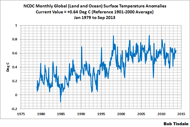
NCDC Global (Land and Ocean) Surface Temperature Anomalies
UK MET OFFICE HADCRUT4
Introduction: The UK Met Office HADCRUT4 dataset merges CRUTEM4 land-surface air temperature dataset and the HadSST3 sea-surface temperature (SST) dataset. CRUTEM4 is the product of the combined efforts of the Met Office Hadley Centre and the Climatic Research Unit at the University of East Anglia. And HadSST3 is a product of the Hadley Centre. Unlike the GISS and NCDC products, missing data is not infilled in the HADCRUT4 product. That is, if a 5-deg latitude by 5-deg longitude grid does not have a temperature anomaly value in a given month, it is not included in the global average value of HADCRUT4. The HADCRUT4 dataset is described in the Morice et al (2012) paper here. The CRUTEM4 data is described in Jones et al (2012) here. And the HadSST3 data is presented in the 2-part Kennedy et al (2012) paper here and here. The UKMO uses the base years of 1961-1990 for anomalies. The data source is here.
Update: The September 2013 HADCRUT4 global temperature anomaly is +0.53 deg C. It increased (about 0.01 deg C) since August 2013.

HADCRUT4
153-MONTH RUNNING TRENDS
As noted in my post Open Letter to the Royal Meteorological Society Regarding Dr. Trenberth’s Article “Has Global Warming Stalled?”, Kevin Trenberth of NCAR presented 10-year period-averaged temperatures in his article for the Royal Meteorological Society. He was attempting to show that the recent hiatus in global warming since 2001 was not unusual. Kevin Trenberth conveniently overlooked the fact that, based on his selected start year of 2001, the hiatus has lasted 12+ years, not 10.
The period from January 2001 to September 2013 is now 153-months long. Refer to the following graph of running 153-month trends from January 1880 to September 2013, using the HADCRUT4 global temperature anomaly product. The last data point in the graph is the linear trend (in deg C per decade) from January 2001 to the current month. It is basically zero. That, of course, indicates global surface temperatures have not warmed during the most recent 153-month period. Working back in time, the data point immediately before the last one represents the linear trend for the 153-month period of December 2000 to August 2013, and the data point before it shows the trend in deg C per decade for November 2000 to July 2013, and so on.

153-Month Linear Trends
The highest recent rate of warming based on its linear trend occurred during the 153-month period that ended in late 2003, but warming trends have dropped drastically since then. Also note that about the early 1970s was the last time there had been a 153-month period without global warming—before recently.
196-MONTH RUNNING TRENDS
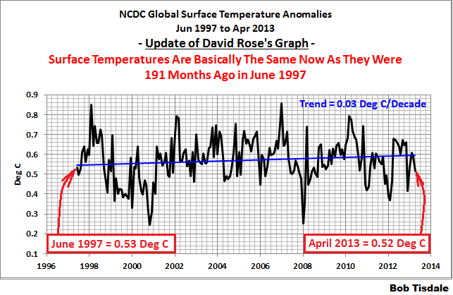
In his RMS article, Kevin Trenberth also conveniently overlooked the fact that the discussions about the warming hiatus are now for a time period of about 16 years, not 10 years—ever since David Rose’s DailyMail article titled “Global warming stopped 16 years ago, reveals Met Office report quietly released… and here is the chart to prove it”. In my response to Trenberth’s article, I updated David Rose’s graph, noting that surface temperatures in April 2013 were basically the same as they were in June 1997. We’ll use June 1997 as the start month for the running 16-year trends. The period is now 196-months long. The following graph is similar to the one above, except that it’s presenting running trends for 196-month periods.

196-Month Linear Trends
The last time global surface temperatures warmed at the minimal rate of 0.03 deg C per decade for a 196-month period was about 1980.
The most widely used metric of global warming—global surface temperatures—indicates that the rate of global warming has slowed drastically and that the duration of the hiatus in global warming is unusual during a period when global surface temperatures are allegedly being warmed from the hypothetical impacts of manmade greenhouse gases.
A NOTE ABOUT THE RUNNING-TREND GRAPHS
There is very little difference in the end point trends of 12+year and 16+year running trends if GISS or NCDC products are used in place of HADCRUT4 data. The major difference in the graphs is with the HADCRUT4 data and it can be seen in a graph of the 12+year trends. I suspect this is caused by the updates to the HADSST3 data that have not been applied to the ERSST.v3b sea surface temperature data used by GISS and NCDC.
COMPARISON
The GISS, HADCRUT4 and NCDC global surface temperature anomalies are compared in the next three time-series graphs. The first graph compares the three global surface temperature anomaly products starting in 1979. The graph also includes the linear trends. Because the three datasets share common source data, (GISS and NCDC also use the same sea surface temperature data) it should come as no surprise that they are so similar. For those wanting a closer look at the more recent wiggles and trends, the second graph starts in 1998, which was the start year used by von Storch et al (2013) Can climate models explain the recent stagnation in global warming? They, of course, found that the CMIP3 (IPCC AR4) and CMIP5 (IPCC AR5) models could NOT explain the recent hiatus.
The third comparison graph starts with Kevin Trenberth’s chosen year of 2001. All three of those comparison graphs present the anomalies using the base years of 1981 to 2010. Referring to their discussion under FAQ 9 here, according to NOAA:
This period is used in order to comply with a recommended World Meteorological Organization (WMO) Policy, which suggests using the latest decade for the 30-year average.
You’ll note that the GISS LOTI data has larger monthly variations than the other two datasets. This is likely caused, in part, by GISS masking sea surface temperature data in the polar oceans and replacing it with land surface air temperature data, which is naturally more volatile. Again, please refer to the discussions here and here.

Comparison Starting in 1979
###########

Comparison Starting in 1998
###########

Comparison Starting in 2001
AVERAGE
The last graph presents the average of the GISS, HADCRUT and NCDC land plus sea surface temperature anomaly products. The flatness of the data since 2001 is very obvious, as is the fact that surface temperatures have rarely risen above those created by the 1997/98 El Niño.

Average of Global Land+Sea Surface Temperature Anomaly Products
As ever, pertinent and informative – thanks for your tireless effort Bob.
‘Hiatus denial’ is becoming increasingly untenable.
The September anomaly of 0.74 C equalled the highest ever recorded in September in the GISS data set, along with 2005. There have been 8 warmer months since 1995, scattered amongst the other months of the year. Four of these were in 2010. The others were in 1995, 1998, 2002 and 2005.
Ooops – missed one. January 2007 can be added to that list.
The big picture seems to be slow overturning toward SST cooling.
I’m guessing there will be a 2007-style La Nina drop in SSTs early next year to conform to ENSO annual phase-locking.
Bob,
The heat will be back. It is currently hiding in the deep oceans and according to Trenberth (or is it Jones?) is conducting hit and run guerilla style attacks in random locations around the world. This year it is causing big typhoons in the western pacific and wildfires in Australia. No one knows where it will strike next.
Anthony,
Something odd with the sea ice page. Some of the arctic and antarctic are linked 3 times in a row. Also some spacing problems early with giant figure running out to margins.
REPLY: Fixed, thanks. NSIDC graphs now back to normal. – Anthony
Two remarks.
* Why is GISS so out of touch with the other two? HADCRUT4 is 0.01C, GISS is 0.13C in one month? I was wondering why and how the Wunderground blog was trumpeting September as the 4th hottest ever — obviously they were using GISS, not HADCRUT4.
This makes little sense, given the [significant] overlap in the underlying data sources for the two, and just as neither one can [increase] without bound to conform to the GCMs via constant “adjustments” because their divergence from UAH/RSS LTT would give the game away even more than it has already been lost, GISS can’t produce warming record headlines relative to HADCRUT4 month by month without causing far too obvious a divergence between the two.
BTW, this is an even better explanation for the wider variance of GISS than the one you offer. If the GISS GASTA varies by tenths a a degree month to month, it is comparatively easy to pick months that “set records” (or come close) even though the trend is neutral. After all, they only get a headline in the media when they set a high temp record, not when it falls 0.1+C the next month to less than the 15 year trend. It is left as an exercise for the audience to compute what fraction of months they can discover as “records” of one sort or another simply by computing their number in such a way that its monthly variance is 0.1-0.2C.
* Sigh… Bob, I know that there is an overwhelming temptation to take three supposedly similar numbers and average them, but it simply is not justified in this or almost any related case in climate science. NCDC, GISS, and HADCRUT4 are three different computations of supposedly the same number, GASTA. They are based on heavily overlapping data. They use different computational methods to e.g. average or smooth the data over spatiotemporal gaps, and they “adjust” the data differently for poorly known or even unmeasurable things such as UHI. They therefore are in no possible sense “independent and identically samples drawn from a common distribution” (iid). Consequently their mean is a meaningless quantity, as is their mutual variance. The Central Limit Theorem does not apply, and neither the mean nor the variance can be taken as reflective of an underlying “true mean” GASTA.
Indeed, all that their difference indicates is that at least two, more likely all three are in error by some unknown amount. This problem is even more pernicious given their substantial data overlap. Given (say) 60 to 80% common data, the averages should be much closer than they are and have very similar noise/variance around an underlying mean. As you do note above, the differences in variance are startling and are actually profound evidence that something is seriously amiss.
I know how tempting it is to assert (or rather, hope) that an average might cancel some of the errors made by each of the three methods, but as long as they share data they are in no sense independent, as long as the are based on differing methodology the are in no sense identically distributed, and there is no theorem or sound argument I can imagine that errors in methodology are unbiased, zero sum white noise drawn from some trendless distribution. Indeed, it is almost certainly not the case that this is so — the REASON that they are able to continually “adjust” the data is that they can assert that they’ve discovered a methodology error with trend.
Again, it is left as an exercise for the audience to compute the probability of (say) 6 successive adjustments for supposedly trended method error that all happen to have the same sign and the same effect, to comparatively cool the past and warm the present, but that’s another story. At this point LTT has put a stop to that. GISS appears to be reduced to desperation — getting headlines at the expense of noise while waiting for a desirable trend in LTT that permits them to observe real trended warming once again. HADCRUT4, after the last round of adjustments, actually appears to be behaving comparatively consistently with NCDC and LTT (finally). Perhaps the era of adjustment driven warming is finally over.
I’m not convinced of this, though. The more I look at correlations from quantities that ought to be correlated with GAST (note well, absolute and not the anomaly) the similarity between the first half of the 20th century and the second is profound. Given that GAST is a completely unknown quantity, I’m wondering how much of the “anomaly” is an artifact. The only thing that prevents me from thinking that it is all is sea level as measured by tide gauges, but recent evidence that a significant fraction of SLR may be caused by subsidence that we are only just barely beginning to measure with universal GPS access is making me wonder even about that. SL SHOULD be the best thermometer we have (at least not susceptible to a UHI that could make the land record increase vanish overnight), and even here we have a pitifully short, pitifully spatiotemporally undersampled reasonably reliable record, especially at depth.
rgb
My guess is an imbalace in percipitation and evaporation, a burst of sensible heat that will radiate away for a net cooling for the next month.
Friends:
In his fine post at October 31, 2013 at 6:40 am, concerning NCDC, GISS, and HADCRUT4 which are three different computations of supposedly the same number (average global temperature), Robert Brown writes
Yes! And this information is not news.
For the benefit of those who have not seen it, I again provide this link and draw especial attention to its Appendix B
http://www.publications.parliament.uk/pa/cm200910/cmselect/cmsctech/memo/climatedata/uc0102.htm
Richard
ie., could differences such as altitude range of observation affect timing of when heat is observed as temperature and explain variance. GISS being at ground level is observing a narrower section of the surface.
Just a quick aside…
It was more of a government ‘slowdown’ rather that ‘shutdown’. Even they stated that essential services were to be maintained. Of course if the others were nonessential why do we have them in the first place.
“Again, it is left as an exercise for the audience to compute the probability of (say) 6 successive adjustments for supposedly trended method error that all happen to have the same sign and the same effect, to comparatively cool the past and warm the present, but that’s another story. ”
the reason is simple. The past was colder than previously thought and the present is warmer.
its not because there is a conspiracy ( we did land on the moon) its because the past was in fact cooler.
If you compute the temperature field correctly you will see this. Any and all improvements to GISS, CRU and NCDC will result in a colder past and warmer current period. Not because they are putting their thumbs on the scale, but rather because the past was in fact colder and the present is in fact warmer.
we even saw some of this this when skeptic jeff ID did his temperature series using a method endorsed by
skeptics.
watch for more on this issue.
in simple terms you have two choices.
1. improvements in methods and data will lead to a cooler past and warmer present
because the past was in fact cooler and the present is in fact warmer
2. Improvements in methods and data lead to a cooler past and warmer present
because every group that does surface temperature averages is corrupt. including
the skeptical Jeff Id.
aaron says: “ie., could differences such as altitude range of observation affect timing of when heat is observed as temperature and explain variance. GISS being at ground level is observing a narrower section of the surface.”
aaron, all three datasets start with the same source data: land surface air temperatures and sea surface temperatures. NCDC and GISS, in fact, use the same sea surface temperature reconstruction. GISS adds some additional data in the Arctic and in Antarctica, but GISS also masks (basically deletes) sea surface temperature data anywhere sea ice forms. That way they can extend land surface air temperature data out over the oceans, and land surface air temperature data are much more volatile than sea surface temperature data.
Regards
Do I have to believe this rising figure?
Robert Brown: I fully understand and agree with you, but there is a logical reason to present the average. That way I don’t have to argue about which one is best.
Steven Mosher says:
October 31, 2013 at 9:39 am
“…the reason is simple. The past was colder than previously thought and the present is warmer.”
Let me see if I can refute this argument, using the same method as Mr. Mosher:
The past was NOT colder than previously thought and the present is NOT warmer!
There…mission accomplished.
Oh…by the way, the future IS cooler than we previously thought.
Glad that is settled.
the reason is simple. The past was colder than previously thought and the present is warmer.
its not because there is a conspiracy ( we did land on the moon) its because the past was in fact cooler.
Dear Steven,
I didn’t say anything about a conspiracy. I made a very simple statement about statistics. Let us assume that nobody in the remote past or present was deliberately trying to make their numbers either “too warm” or “too cold”. Errors from all sources — miscalibration of thermometers, reading temperatures inconsistently, poor placement of thermometers, and so on would in general be assumed to be as likely to be too warm as too cold. This is as true in the modern era as it is in the remote past. If one is correcting the record in the past, then, it should be just as likely that the correction required be negative as it is positive. If one is correcting the record in the present, it should be just as likely as that the correction be negative as it is positive. On average, one would a priori assume that while any given error one discovers might alter the overall trend up, the corrections for many errors should be as likely to alter it up as to alter it down and (within the usual square root associated with a random walk) should be zero mean, trendless.
We can thus assert the null hypothesis: All the corrections made to computed estimates of GASTA are honest and unbiased. Our prior assumption (in a strictly Bayesian sense) is that corrections are a coin flip, equally likely to increase trend as decrease trend. We could go further and talk about an actual distribution of corrections within some probable range, but let’s keep it simple with coin flips. The data is then we flip a coin six times in a row and get heads every time — every correction creates more relative warming, some of them rather significant relative warming. Does the data support the null hypothesis?
Of course not. In fact, the p-value for getting 6 heads in a row is only 1/128, much less than 1%. The probability of getting 6 corrections that all increase the warming trend in a row is (given the prior of unbiased corrections equally likely to increase or decrease trend) sufficient to reject the null hypothesis and state that it is rather likely to be the case that the prior probability of the coin flip is not, in fact, 0.5, but instead that the probability of getting heads (or a systematic increase in trend) is indeed significantly more than 0.5.
Nicholas Nassim Taleb describes this circumstance quite clearly in his lovely book, The Black Swan where he has a scientists (like yourself) and a cab driver named Joe analyze the probability of flipping just such a coin and getting just such an improbable string of heads. The scientist is asked to compute the probability of the coin coming up heads on the next flip, and of course answers 0.5, because it is a two sided coin and the coin flips are independent trials, so it is just bad luck that it came up heads so many times in a row. Joe the cab driver replies quite differently: “It’s a sure thing you’ll get heads. It’s a mugs game — the coin is fixed.”
A Bayesian agrees with Joe. A Bayesian isn’t certain that the coin is fixed, not from only six flips, but is definitely lifting an eyebrow and thinking “Oh, really?” Then we could go down the line on many more flips in climate science where the bread lands butter side down, where “adjustments” or “errors” somehow always seem to increase the warming trend but never decrease it.
Finally, one really has to ask how you know this: “the past was in fact cooler”. Are you somehow gifted with second sight so that you just “know” precisely what GAST was (within the tenths of a degree Celsius necessary to support all of the vast range of conclusions that are being made about global warming and its causes) so that you can state that it was in fact cooler? Can you be very helpful in that case and tell me how much more cooler it will end up after GISS and HADCRUT4 etc make their next set of “corrections”? Would you explain how your knowledge apparently exceeds the stated/acknowledged probable errors (which are generally presented, BTW as being symmetric and hence suggest that even the creators of HADCRUT (for example) believe their uncertainty is unbiased and symmetric — except when it comes to making a correction that is supposedly a part of that error)?
Personally, I have to say that the notion of “correcting” a data set long after the fact is a process so fraught with the opportunity for error and bias that most angels quite rightly fear to tread there. We wouldn’t tolerate it for a minute in biological research or health care, because there we have ample direct evidence that people simply cannot avoid making all “corrections” to their data improve their confidence in some desired or profitable conclusion. Obviously you have tremendous faith that this does not happen in climate science, even though it obvious is just as likely to actually happen there as it is to happen anywhere else somebody isn’t forced to double-blind their data and not adjust it once they begin analysis. You persist in this belief even though the observed series of corrections is highly improbable given presumably symmetric errors as reflected in the symmetric error bars assigned to the curves. You, my friend, are playing a mug’s game, at least according to Joe the cab driver.
I’m just sayin’.
rgb
As GISS temp numbers always change in later issues it is safe to admit that they are wrong (and ignore them).
I look at the exercise at looking at GISS temp numbers from the perspective of recording historically how these are, and how these will change.
If one looks now at the LOTI maximum values, there are peak values in the years 1998, 2002, 2007 and 2010.
One can look at these and predict how these will evolve in future issues.
We can see now the 2010 peak being lower then the 2002 peak.
Next year 2002 will decrease and be at the same level with 2010. By the end of 2014 the 2010 value will be higher then the 2002 peak. Simply as that.
By 2015 the 2010 temp value will catch up with the 2007 value, with 2002 being a clearly lower value in the continuous increase of temperatures.
So what other use is looking at GISS temp?
Even if now thinking at it, maybe one could write a paper about temporal heat transfer – based on GISS data….
Well, I will bookmark this link for later reference…. & just having fun…
Sorry Bob for this but I cannot take GISS serious.
Steven Mosher says:
October 31, 2013 at 9:39 am
the reason is simple. The past was colder than previously thought and the present is warmer.
its not because there is a conspiracy ( we did land on the moon) its because the past was in fact cooler.
If you compute the temperature field correctly you will see this. Any and all improvements to GISS, CRU and NCDC will result in a colder past and warmer current period. Not because they are putting their thumbs on the scale, but rather because the past was in fact colder and the present is in fact warmer.
Wow this is low…
And because we landed on the moon we will see the relative value of 2010 getting warmer then 2002 in the future and because the past was colder we will see 2002 getting colder. Right Steven.
Continuing with the probability theme, what is the probability that Hadcrut4 for September 2013 is exactly the same to the nearest 1/1000 degree as September 2012, namely 0.534 and that Hadcrut3 was 0.516 for both 2012 and 2013 in September? Or was there a mistake here?
the reason is simple. The past was colder than previously thought and the present is warmer.
I’m glad that you know this, for a fact. I’m very interested to know how you know this, for a fact.
Additionally, even assuming that the past was cooler and the present is warmer, why wasn’t one adjustment enough? Why are there continuing adjustments every couple of years, with each of them making the past ever cooler and the present even warmer?
With regards to GISS and Hadcrut4, check out the stats for this year. In 5 of the 9 months so far, GISS and Hadcrut4 went in opposite directions. It is almost as if they are doing different planets.
http://www.woodfortrees.org/plot/gistemp/from:2013/plot/hadcrut4gl/from:2013
I could see averaging RSS (or UAH) and Hadcru (or NCDC). They are measuring different things and they are independent.
As for Mosher’s comment …. well, it appears he knows exactly how to factor in urban heat islands, airport heat islands, agricultural heat islands, siting problems, missing “M” coding, atmospheric mixing due to large structures, land use changes and researcher bias (to name just a few). What a mental giant.
I could read RBG brilliant posts all day to be honest. Everyone interested in global warming climate change 7 maths and physics should read about “Climate as a random walk” as a model fit its much much better than anything else. This really simple WM Briggs post is brilliant
Especially Steve Mosher.
Its a really hard concept to get your head around, but the maths are really simple.
http://wmbriggs.com/blog/?p=257
I could read RBG brilliant posts all day to be honest. Everyone interested in global warming climate change 7 maths and physics should read about “Climate as a random walk” as a model fit its much much better than anything else. This really simple WM Briggs post is brilliant
If you like that, you’ll like the work of Koutsoyiannis even better. It isn’t actually best fit by a random walk, but by a Hurst-Kolmogorov process of punctuated equilibrium. It isn’t clear that the steps are trendless and unbiased, although they could be — this is enormously difficult to determine from comparatively short stretches of data. Bob Tisdale’s SST data makes this overwhelmingly obvious, and he identifies ENSO events as a trigger for the jumps, but that still doesn’t yet predict the direction of the jumps or their magnitude (that is, the long term underlying trend in the local equilibria the jumps move between).
The mathematical model for this is probably a space of local attractors with complex poincare cycles moving the climate around them, and with events or just plain time evolution causing comparatively sudden “jumps” between attractors. The motion and structure of the underlying attractor space, however, is largely unknown. I don’t even think we know the dimensionality of the space. What we see in GASTA is at best a projection onto a single axis of a complex motion around and between locally stable points.
rgb