From Dr. Roy Spencer’s Global Warming Blog
Roy Spencer
July 3rd, 2025 by Roy W. Spencer, Ph. D.
The Version 6.1 global average lower tropospheric temperature (LT) anomaly for June, 2025 was +0.48 deg. C departure from the 1991-2020 mean, down slightly from the May, 2025 anomaly of +0.50 deg. C.

The Version 6.1 global area-averaged linear temperature trend (January 1979 through June 2025) now stands at +0.16 deg/ C/decade (+0.22 C/decade over land, +0.13 C/decade over oceans).
The following table lists various regional Version 6.1 LT departures from the 30-year (1991-2020) average for the last 18 months (record highs are in red).
| YEAR | MO | GLOBE | NHEM. | SHEM. | TROPIC | USA48 | ARCTIC | AUST |
| 2024 | Jan | +0.80 | +1.02 | +0.58 | +1.20 | -0.19 | +0.40 | +1.12 |
| 2024 | Feb | +0.88 | +0.95 | +0.81 | +1.17 | +1.31 | +0.86 | +1.16 |
| 2024 | Mar | +0.88 | +0.96 | +0.80 | +1.26 | +0.22 | +1.05 | +1.34 |
| 2024 | Apr | +0.94 | +1.12 | +0.76 | +1.15 | +0.86 | +0.88 | +0.54 |
| 2024 | May | +0.78 | +0.77 | +0.78 | +1.20 | +0.05 | +0.20 | +0.53 |
| 2024 | June | +0.69 | +0.78 | +0.60 | +0.85 | +1.37 | +0.64 | +0.91 |
| 2024 | July | +0.74 | +0.86 | +0.61 | +0.97 | +0.44 | +0.56 | -0.07 |
| 2024 | Aug | +0.76 | +0.82 | +0.69 | +0.74 | +0.40 | +0.88 | +1.75 |
| 2024 | Sep | +0.81 | +1.04 | +0.58 | +0.82 | +1.31 | +1.48 | +0.98 |
| 2024 | Oct | +0.75 | +0.89 | +0.60 | +0.63 | +1.90 | +0.81 | +1.09 |
| 2024 | Nov | +0.64 | +0.87 | +0.41 | +0.53 | +1.12 | +0.79 | +1.00 |
| 2024 | Dec | +0.62 | +0.76 | +0.48 | +0.52 | +1.42 | +1.12 | +1.54 |
| 2025 | Jan | +0.45 | +0.70 | +0.21 | +0.24 | -1.06 | +0.74 | +0.48 |
| 2025 | Feb | +0.50 | +0.55 | +0.45 | +0.26 | +1.04 | +2.10 | +0.87 |
| 2025 | Mar | +0.57 | +0.74 | +0.41 | +0.40 | +1.24 | +1.23 | +1.20 |
| 2025 | Apr | +0.61 | +0.77 | +0.46 | +0.37 | +0.82 | +0.85 | +1.21 |
| 2025 | May | +0.50 | +0.45 | +0.55 | +0.30 | +0.15 | +0.75 | +0.99 |
| 2025 | June | +0.48 | +0.48 | +0.47 | +0.30 | +0.81 | +0.05 | +0.39 |
The full UAH Global Temperature Report, along with the LT global gridpoint anomaly image for June, 2025, and a more detailed analysis by John Christy, should be available within the next several days here.
The monthly anomalies for various regions for the four deep layers we monitor from satellites will be available in the next several days at the following locations:
It was the second warmest June in the UAH record, after 2024.
Moyhu.s TempLS surface temperature was similarly down 0.047C. Here is the map:
0.047 degrees?
That’s a lot of precision. The temperature of my room can’t be given to 0.001 degrees precision, as it varies by much more than than from one spot to another.
I’m not criticising Nick’s post. I’m just wondering what it means in reality to give that kind of number as the change in temperature.
Your room isn’t the world. 0.047 is not a thermometer reading. It is the outcome of a calculation based on thousands of thermometers around the globe.
When you calculate a number, you should express it to whatever precision anyone is likely to want. Then they can argue about uncertainty, but they know what your calculation found.
Sorry, but you wouldn’t pass high school physics or chemistry with metrology skills like that. You could measure a boiling beaker of water a million times with 100 thermometers or probes but in the end you not allowed to quote numbers to 6 digits if the tools are only good to 2 or 3.
And that is many magnitudes more true when measuring the “temperature of the Earth” with instantaneous probes with no time averaging, disparate and unevenly spread out locations, locations that fail measurement standards, infilling of data to a ridiculous degree… and on and on.
Dr. Spencer’s work and that of his satellite colleagues is very commendable for eliminating the concerns above.
However I don’t think any of the climate scientists are measuring the changing climate but really the urbanization effect.
Yet Dr Spencer’s data set has been warming at the same rate as the GISS and NOAA surface data sets over the past 20 years; both +0.31C per decade.
And there is no evidence in the UAH data of anything but warming at naturally occurring El Nino events.
If you think there is warming by human released CO2, then identify it in the UAH data, and give a value to it.
And it is absolutely impossible to show any CO2 warming in the surface data… it is way too corrupted by urban and site degradation.
If a particular hypothetical forcing is rising essentially continuously, but the variable that is claimed to be affected is only showing episodic transient increases at 3 or 4-year intervals, then it is time to revise the hypothesis.
Year to year radiative forcing changes are small and easily swamped by short-term variability. But over the long term, that variability averages out. What remains are the persistent forcings, like greenhouse gases and aerosol reductions. That’s why we see long term warming. So the short term fluctuations you point to don’t falsify or even challenge the mainstream explanation.
The logic in your comment is akin to walking on a treadmill that is gradually speeding up, but the moment it slows down slightly, you insist it is broken.
That’s very scientific! Wow!
Yes, CO2 warming goes on vacation after each El Nino event.
It no more goes on vacation than does the x term in y = x + sin(2x) in the portion of the graph that declines (dy/dx < 0). The x term is still there driving a long term increase in the graph. It’s just that the sin(2x) term is also acting to create short term variation that manifest as a decline in the graph on occasion.
This is referred to as the reduction fallacy. This fallacy is the result of assuming that one and only one independent variable is influencing the dependent variable.
I created the following model with 5 independent variables primarily to help people visualize how multiple factors can stack (or superimpose) on one another to create a complex ebb and flow in the dependent variable (UAH TLT) despite the fact that only one of the independent variables (CO2) is continuously increasing.
As a matter of interest, how well does that fit to, say, the GISS or HadCRUT data?
It’s a good question for which I don’t have a good answer at the moment. I’d have to train the model on the surface datasets first. That’s not something I’ve done yet.
What training would be involved? Shouldn’t it just be a matter of using the same weightings on the GISS, HadCRUT or ERA data sets?
Training the model on the other data sets is a bit too much like von Neumann’s elephant.
The surface datasets are not measuring the same thing as UAH TLT. The weightings will be different because the surface temperature does not behave the same as the lower-to-mid troposphere temperature.
It is like Neumann having both a Loxodonta africana and Elephas maximus and developing separate models for each. Sure, they’re both Elephantidae, but with enough differences that they can be classified not only as separate species, but as separate genus too. A model for one should not be expected to completely explain the other.
But the point of model overfitting is still good nonetheless. Just because the model above fits UAH TLT with an R^2 = 0.78 does not necessarily mean that it will maintain that level skill against big swaths of future data points for which the model was not trained. That’s one of the problems with machine learning in general…overfitting. But again the intent of the model isn’t to prove causation. The intent is to falsify the hypothesis that 1) CO2 is not correlated with UAH TLT and 2) the ebb and flow of UAH TLT is inconsistent with CO2 models because CO2 increases consistently and monotonically.
That’s an interesting point. Apart from a different offset in absolute temperature (negated by using anomalies) and some attenuation due to conduction and convection, should there be much difference in response between the surface and lower troposphere?
What causes different temporal response patterns?
That might be an interesting research area.
That’s the first rule of time series analysis: “Though shalt not extrapolate” 🙂
Actually, that’s somewhat over-generalised. You mostly get away with it because of strong autocorrelation, but when you don’t it can bite hard. We were in the middle of a semester-long uni exercise involving stock prices , when one of the major crashes occurred in the late 1980s
I wasn’t really thinking about the offset between datasets to be a fundamental difference in this context so it is easily corrected with a constant. I was thinking primarily about the ENSO response. The last time I did this exercise with the surface datasets I was getting a 3-month lag as opposed to a 5-month and with a lower magnitude in the response. This seems to be reasonably well known difference.
One of things I was proactive about was avoiding higher order terms (x^2, x^3, etc.). I think a lot models move too close to the overfit side of the spectrum when they use higher order terms. That’s not to say that I think this particular model can’t at least partially indicted of overfitting. Afterall, most models in this form have at least some element of it if people were being honest.
That’s interesting. I wonder why the lag is different.
What a load of waffle.
Extraordinary claims require extraordinary evidence.
If you want to convince me that combining 2 or more variables exhibiting a cyclic behavior with a another variable that monotonically increases cannot produce an output that is itself monotonically increasing then present extraordinary evidence.
The problem is that CO2 (your monotonically increasing variable) displays that behavior over a long period of time, i.e., an average. These are all time series of continuous variables that have their own periods and amplitudes. You can’t just average their behavior and say “look”.
You would need to do a Fourier or wavelet analysis to determine each piece part of each variable to get a picture of what is occurring on a continuous basis.
I’m coming in late on this conversation, but (puts consultant statistician hat on) this is exactly the approach to be taken. Would love to chat offline about how to refine models like this.
It’s clear CO2 is playing some part in global temperatures, but it’s only part of the story.
It is clear?
Again, the nonsensical disregard for the cooling effect of La Nina on display.
Thanks for producing ZERO evidence of CO2 warming in UAH. 🙂
What are you even talking about?
TFN says: ‘Again, the nonsensical disregard for the cooling effect of La Niña on display.’
And you somehow think that backs up your point? How?
Some deniers are down right stupid.
Well, that’s irrelevant word salad, isn’t it? You believe in a GHE which you can’t describe, and ignore currently known laws of physics.
That would make you ignorant and gullible.
The greenhouse effect does exist.
Is this the greenhouse effect that you can’t describe in any consistent and unambiguous way, or some other imaginary greenhouse effect?
Maybe you could claim that you aren’t really ignorant and gullible. Somebody might believe you.
Nobody rational, of course.
Someone who does not understand their own argument should be wary of pointing fingers.
No, the La Niña is just an observed pattern of temperatures. You believe otherwise, but your belief is not rational.
La Nina is not a cooling per se.
La Nina is the absence of heating the atmosphere.
El Nino heats up the atmosphere by pumping water vapor into the atmosphere. A temperature effect most noticeable at night and in the winter.
Otherwise, the CO₂ effect would be consistent with CO₂’s ppm increases.
It isn’t!
CO₂’s temperature signal is indistinguishable from any other trace input source.
Complete nonsense, unfortunately. Adding water vapour to the the atmosphere creates no heat whatsoever. As a matter of fact, the hottest places on Earth are those with the least water vapour in the atmosphere – places like Death Valley and the Lut Desert.
Someone is playing you for a fool if they have convinced you that El Niño is anything other than a name given to a pattern of observed temperatures.
Warming – if you want to call it that – is occurring at the El Nino events as step-ups. La Ninas do not have the ”cooling” effect that you are talking about but a moderating effect from the EL Nino peaks. As you would expect, warming would not be linear but most likely just as we are seeing. In fit’s and starts. You cannot deny that warming is occurring at El Ninos, but not necessarily because of them. Generally, the temp settles down slightly higher after El Nino events. They are not the cause but part of the mechanism. The cause is ocean overturning cdriven by the sun with possibly decades of lag. Nothing to do with CO2.
”
Comprehension problem?
The Version 6.1 global area-averaged linear temperature trend (January 1979 through June 2025) now stands at +0.16 deg/ C/decade”
Which part of “the last 20 years” don’t you understand?
As I made clear (but not to everyone, apparently), I was referring to the last 20-years for comparison purposes.
Where there has been two strong El Nino events.
How much of that El Nino warming was caused by CO2 ?
Waiting for an answer.
probably about 0.0001 degrees. Give or take a zero.
Comparing two different measurement models is not science. NOAA shows a ±0.3°C uncertainty for CRN station measurements, the best in the world that use an average of 3 thermometers in the same aspirated housing at 2m altitude.
Using a +0.31°C ΔT as a point value for the center of an interval makes the uncertainty interval at least [0.0°C to +0.6°C]. That means the real value could be as low as 0.0°C or as high as +0.6°C with no way to choose any temperature between the end points.
That interval is also assuming that all stations on the globe are as accurate as USCRN stations. Remember, NOAA publishes the uncertainty of ASOS (next best) stations as ±1.8°F (±1.0°C). Many MET stations, as pointed out here on several threads, have uncertainties of +2 to +5°C.
To be scientific, one must always include the uncertainty interval when quoting the point value of a measurand. Dr. Spencer, GISS, and NOAA would do well to follow that practice. The lack of an uncertainty being quoted makes the result appear unscientific.
From the JCGM 100:2008.
When the uncertainty is not quoted, there is no ability to evaluate the specificity of the measurement.
And one loses a sense of the variance in the data because in using mid-range averages (median of diurnal extremes) one doesn’t know whether there is a small range or large range because the mid-range can be the same for either.
You’re not wrong. But I think the concern at least in regard to how it may effect the global average temperature trend is unwarranted since other datasets (like ERA provided by Copernicus) use more rigorous averaging methodologies that do not depend on the diurnal extremes. Those datasets show a similar amount of warming as compared to the datasets using the (Tmax+Tmin)/2 method.
Maybe it’s just a coincidence that global warming in UAH has risen at exactly the same rate as it has in GISS and NOAA over the past 20-years, despite the fact that they measure different parts of the atmosphere.
Do you understand the difference between coincidence of measurement of different measurands and the same measurand? How about the difference between 2m and 5000m.
They ARE two different measurement models of different measurands. Any coincidence is pure luck.
coincidence could also be by design as well as luck.?
“by design “
With so much junk surface data, they can get any result they want. 😉
The difference in the GISS and NOAA data and the UAH data is the UAH data did not show a “hottest year evah” (one hotter than 1998) until 2016, yet GISS and NOAA were proclaiming “hottest year evah!” for year after year from the year 2000 until 2016, about 10 different time, if I recall correctly, and GISS and NOAA even went so far in their data bastarization to present one year after another as being hotter than the previous year.
None of that Alarmist Climate Change Propaganda can be found in the UAH chart. NO years after 1998, were hotter than 1998 until the year 2016 was reached, where 2016 was one-tenth of a degee warmer than 1998.
The UAH chart is in this article. Show me one year between 1998 and 2016 that was hotter than 1998. There are no such years.
GISS and NOAA had to beat their computers realy hard to continue the lies they told about the temperatures after 1998.
Hansen was stunned when the temperatures started cooling after 1998. He figured all along that the temperatures would continue to rise because CO2 was continuing to rise, but, Surprise! Surprise!, the temperatures cooled, so the Climate Alarmists in our government decided they needed to start mannipulating the data so they could continue the CO2-crisis Lie.
Yeah, look at the UAH chart. GISS and NOAA claim 10 years between 2000 and 2016 were hotter than the previous years.
The UAH chart shows GISS and NOAA are Climate Change Liars. The mannipulated the data for political purposes. Science Fraud.
As UAH did for 2023 and 2024?
Apparently you have a selective memory.
Indy cars and Top Fuel dragsters can reach similar speeds yet they do so very differently. Most people would admit they don’t know the intricacies of each. You, on the other hand, would say you KNOW the differences because you can read correlations and determine the casual variables.
Over the course of the race, do they finish at exactly the same time? Because that is the analogy we have when comparing UAH and the surface data.
.16 C per decade stated under graph.
“However I don’t think any of the climate scientists are measuring the changing climate but really the urbanization effect.”
Then why is UAH showing virtually the same trend in the warming of Earth’s atmosphere?
It measures a section of the atmosphere centred at 4km.
Also it cannot see the nocturnal warming at the surface under low level inversions, where the GHE shows up the most.
Nocturnal warming at surface sites is UHI effect.
That’s why it shows up most in urban areas.
UAH is measuring the surface of the Earth just like with the thermometers, so why wouldn’t it measure UHI effect? Look at the big difference between land and sea measurements.
First…why do you not want it to measure the UHI effect. The UHI effect is real. That is warming that really occurred. As such it is desirable for UAH to include it if it influences the TLT layer that they are measuring.
Second…you may be confusing the UHI effect with the UHI bias. Those are different, albeit related, concepts. As I said above the effect is real so it is preferable that it be included. The bias is not a real effect. It is an artifact of the spatial sampling, infilling, and average methodology. UAH’s methodology is mostly immune from the UHI bias.
UAH-Land is has about 1.5 x the trend of UAH-Oceans, hot are rises, so there is some small leakage of the UHI effect into the UAH data.
And thanks for admitting that surface warming is strong affected by urban heat…
… (as well bad sites, and data fabrication and manipulation)
The slower trend is due to the thermal inertia of the oceans. Land heats faster than water, for crying out loud.
Yet you’re claiming El Nino causes global warming while not even grasping the basic concept of oceanic heat lag.
You have FAILED yet again to make any case for CO2 warming.
Great that you seem to comprehend the warming from El Nino events , though
UAH-Land is the atmosphere above the land.
UAH-Oceans is the atmosphere over the ocean….
The El Nino warming effect comes FROM the oceans.
….. for crying out loud. !!
And yes, ocean heat lag is what causes the step change at each major El Nino event, as warmer water is transferred to adjacent basis.
You have yet to show any CO2 warming in the UAH data.. or to put a value to it.
Expanding on this further…it would not be unreasonable to hypothesize that if anything UAH could actually have a negative UHI bias since they tend to disproportionately oversample non-urban areas due to the way the satellites orbit the Earth and where urbanization has tended to occur.
If (and that’s a big if) this is the case I suspect the bias would be negligible because 1) the oversampling of non-urban areas could be relatively small, 2) Dr. Spencer’s UHI dataset shows that the UHI effect itself contributes only a few hundreds of degree C to the global average temperature rise, and 3) this effect would wash out through the thick TLT layer.
This would be an interesting line of research for one of the experts to tackle.
No, it’s measuring the atmosphere at various heights.
Indeed. Quite a few people assume that it does. That is why i take Spencer’s chart w a grain of salt. It can be combined w other charts for comparison but this whole lower troposphere temperature modeling still leaves me rather lukewarm. People can (and do) make of it what they will. It signifies very little given the variations in atmospheric pressures and their impact. Averaging them out does imo not signify or indicate anything useful.
But i enjoy all the nitpicking to and fros about it..
🙂
To add: i have watched myself dabble into this ‘debate’ on occasion. I see it as playing out in a virtual courtroom without a judge or witnesses, where the prosecution and defense argue about various points that often do not overlap.. The questions and answers often do not correlate and people start throwing mud and deliberate insults to see if the other side is thrown off balance.
It is the online playground. I try (and fail at times) to steer clear.
It’s funny that the Spencer graph often attracks hundreds of comments as if the starting pistol has gone off and exactly the same to and fros are drawn out again. Talking about a dead horse: keep on flogging, guys. You get ZERO points and everybody loses.
And verified via weather balloons.
Ghost hunters hunt ghosts at night because you can’t see ghosts in the daytime.
Ghost hunters can’t see ghosts night or day. A complete irrational claim by Phil.
Which is why the purported professionals set up recording apparatus and cameras for days, looking for any sign of an assumed spirit.
Independent satellite and surface temperature datasets agree more than they disagree. Also, if global temperature uncertainty were truly large, wouldn’t signals like ENSO get drowned in noise? They don’t. The peaks and troughs of each ENSO cycle are always resolved.
“The peaks and troughs of each ENSO cycle are always resolved.”
Yep, and there is no evidence of any human CO2 causation whatsoever.!
The only warming comes at those El Nino events.
ENSO produces nice distinct signals, usually about a whole degree in a short amount of time. The rest of the temp increase is small and doesn’t seem to care about the actual amount of CO2 added. And why is Mars experiencing the same kind of climate change? Is the pollution from Chins and India, etc., so bad it’s reaching there?😜
And just like that, you deflect to a completely different topic. Appreciate the confirmation that your claim about measurement uncertainty was never defensible. It sounds like a talking point you picked up without thinking it through.
Well, we are still waiting for evidence of a ‘runaway’ GHE, as it should have by now. Either CO2 does significant ‘forcing’ or it doesn’t. I am always amused by the CO2= forcing people to hear them state other factors are influencing temperature when a graph goes down but then state that it goes up because of CO2. There is really no point in further argueing..
Do surface temps show no warming for 40 odd years beginning in 1968 and earlier?
“metrology”
This is not metrology. It is calculation of a global average. There is no measuring instrument for that.
No, it’s a fantasy and completely meaningless. The Earth has cooled to its present state, in accordance with known physical laws.
Sir Isaac Newton calculated very precisely the size of New Jerusalem. You surely wouldn’t challenge the accuracy of his calculations, would you?
Calculations are worthless if based on fantasy. Averages are often the refuge of the ignorant and gullible.
That’s an opinion, and not one shared by any major scientific institute, nor by Roy Spencer and co at UAH, apparently.
But we’re all entitled to our opinions, including the daft ones.
I’ll point out to you, as I did to Nick Stokes, NIST (National Institute of Standards and Technology) Technical Note 1900 Example 2 provides a method of calculating a point value and uncertainty of series of daily Tmax temperatures.
This post, of all the ones you make, best epitomizes your lack of knowledge in making scientific physical measurements.
“But we’re all entitled to our opinions, including the daft ones.”
Try some introspection 😉
Why should I care about the opinions of unnamed “major scientific institutes”? You can’t even say what this “global average” means, in physical terms. Surface temperatures vary between about 90 C and -90 C. The average is zero.
The undefined and flexible “global average” beloved of GHE believers is a useless fantasy – unless you can demonstrate otherwise, of course.
Opinions ain’t worth spit, as they say.
Indeed. They obviously don’t care about yours.
Exactly. Like mine, all their opinions (plus $5 cash) will buy a $5 cup.of coffee.
90C?
OK, so I’m conservative.
Yes, Precision over accuracy. Thanks for that. Instrument accuracy cannot be averaged. They remain true for each individual instrument over each individual reading. And that doesn’t take into account instrument drift. 😉
What does this even mean?
The numbers you get from instruments are just numbers, like any other numbers. Of course they can be averaged.
Instrument drift is taken into account by UAH.
But it has no signification to average these measurements.
Averaging temperatures is as meaningful as averaging telephone numbers.
Only for as long as that particular instrument remains in the field.
Unfortunately, people who maintain the equipment will swipe out one instrument for another without dual measurements over time!
“What’s in that MMTS Beehive Anyway?
The maintenance article mentions mammals, insects (wasps, bees), contaminants being inside the temperature station that affect it’s accuracy.
Maintenance described, staff pick up the old beehive and plug an entirely new on in it’s space.
Making individual temperature stations not only plagued by contamination but by different equipment taking the temperature.
Great article! It gives a good description of what field instruments go through. Hauling around oscilloscopes, VTVM’s, etc. in the field, regardless of how careful you are, is not conducive to accuracy.
This doesn’t even address changes in the station infrastructure itself over time. Things like paint and UV impacts, calibration drift due to continuous heating and thermal effects on the pieces and parts, and changes to the microclimate such as trees getting taller and wider.
Which is why climatology will always be nothing more than a liberal art and not a physical science.
It is calculating, however it violates most of the criteria that is required for those calculations to be meaningful.
So you are confirming that the numbers are just made up?
Just curious then where you get the numbers that you’re calculating the global average from?
Stated on the map I showed. GHCN V4 and ERSST V5.
The map you show has no uncertainty shown for the values displayed. Does that mean there is none?
If the average is based on measurements and the result is used to “calculate” a temperature and even a ΔT temperature, then you and others are incorrectly labeling it a temperature.
I would point out that NIST accepts both the mean and standard deviation of daily Tmax as statistical parameters in NIST TN 1900. NIST uses these parameters to determine the uncertainty of the point value in an interval.
Maybe you should begin a conversation with Dr. Possolo at NIST about why they consider the mean of a number as a measurement rather than a plain old high school average of a set of 100% accurate numbers.
Yes GAT is a construct full of assumptions, not a measurement.
So again, PROBITY is woeful.
UAH uses time averaging.
UAH uses disparate and unevenly spread out locations.
UAH infills data up to ~4170 km away spatially and 2 days away temporally.
UAH does all of those things.
In other words zero.
The idea that averaging two thermometers can give you an accuracy greater than either thermometer is something so stupid that only a climate scientist could come up with it.
And no, precision is determined by the capability of the equipment you are using, not by what your customers want.
This has been explained dozens of times to Stokes, ToeFungalNail, Phil and the others, but it never goes in through their thick skulls.
You can get an extra digit – say when you eyeball the thermometer between two different degree markers but that’s it. With probes all those digits on the screen makes scientists overconfident in their numbers and prone to overlooking the exhaust fan or car exhaust blowing near the Stevenson screen.
You can get more than one digit. It depends on the specific measurement model and the correlation between inputs. For example, a measurement model with a partial derivative ∂y/∂x_i = 1/n for all x_i from 1 to n and r(x_i, x_j) = 0 then u(y) will have a result 2 decimal places to the right relative to u(x_i) when n = 10000. Refer to equation 16 in [JCGM 100:2008].
Yet again bgw abuses the GUM to get the answer he wants.
And once again, calculating an average is not a “measurement model”.
Using statistical means to reduce measurement uncertainty is only valid for multiple measurements of the same thing. Using the same instrument.
Says who?
Says the JCGM Guide, which you’ve been told again and again but refuse acknowledge.
WUWT lets us use links. Please do as I do, and insert the link, lead us to the reference, and ideally c/p it.
Per the rules of superterranean view exchange, it is first up to Mr. McGinley to back up his claim. But since you have claimed that the “same instrument” whimsy is backed up in the JCGM Guide without saying where, that same rule applies to you. Pray elucidate…
If you were familiar with metrology you would not need to be led to this. The GUM, JCGM 100:2008 is the Bible of metrology.
But to satisfy you search for knowledge here is a definition.
We all agree on what measurement processes we’ll have available in Heaven. Sorry that you missed the “in many cases” part. Now, show me where in the GUM we need to disregard the steadily improving, real world measurement processes that are used in manufacturing, medicine, engineering, around the world, pretty much forever.
You’re obviously an Engineer In Name Only. If you had actually practiced, then you would know that we:
OTOH, E’sINO like you use the excuse that we don’t yet have the Heavenly Answer to freeze in place*. You are the bane of business and science.
“steadily improving, real world measurement processes “
When those are “averaged” with 100 year old measurement processes the measurement uncertainty is dominated by those 100 year old measurement processes. Or pick 50 years ago. Or 20 years ago.
You seem to be unable to grasp that the measurement uncertainty of even current temperature measurement stations range from 0.3C to 0.5C. You simply can’t take measurements with a 0.3C measurement uncertainty and determine differences in the hundredths digit. The measurement uncertainty subsumes the difference you are trying to identify!
And the 0.3C to 0.5C intervals are the inherent calibration measurement uncertainties. The interval doesn’t include the measurement uncertainties that come from different microclimates for different station environments.
Even satellite measurements suffer from the uncertainties introduced by variable path loss of the radiance they are measuring as the satellite travels around the earth. No amount of averaging or parameterization can remove that inherent measurement uncertainty. That unknown alone legislates against an accurate estimate of temperature to the hundredth of a degree.
Error is not uncertainty.
Uncertainty increases as individual measurements are combined.
Sorry that metrology has left you in the dust.
Are you ever going to explain what you think uncertainty is, rather than just saying what it isn’t?
“Uncertainty increases as individual measurements are combined.”
Define what you mean by “combined”. I assume you are talking about an interval/set theoretic interpretation of uncertainty. But even then uncertainty does not increase as you combine measurements into an average?
“Sorry that metrology has left you in the dust.”
I’ve seen no metrological texts that suggest using interval arithmetic, except as a worst case upper limit. Usually they use probability theory.
Been there, done that.
If you wish to remain ignorant of reality, all for the sake of your CAGW party line, I cannot stop you.
It’s all right, I didn’t expect you could answer, but it was worth a try.
Don’t bother. None of them can convincingly answer the question: if the uncertainty is really as large as they claim, then why do so many independent datasets and metrics still broadly agree with each other?
https://wattsupwiththat.com/2025/07/06/uah-v6-1-global-temperature-update-for-june-2025-0-48-deg-c/#comment-4091309
I mentioned this in another thread, but take a look at CERES satellite data—which measures absorbed shortwave radiation completely independently from surface temperature measurements.
Figure 7 in this paper shows a strong correlation between absorbed solar flux and global surface temperature anomalies, with a consistent lag of 0 to 9 months. That suggests a clear, physically meaningful relationship:
https://www.mdpi.com/2673-7418/4/3/17
And yet, we’re supposed to believe the uncertainty is too large to draw any conclusions? Tim insists that the uncertainty is so significant that we can’t even tell the sign.
Then do write down what you believe the real uncertainty limits are.
Don’t just hand-wave.
Very small. Climate science has the right answer. Pat is wrong.
Got any citations for your claim?
I’ve given you plenty of evidence already. You’re just choosing to ignore it.
You ignore stuff like this:
https://wattsupwiththat.com/2025/07/08/climate-oscillations-7-the-pacific-mean-sst/#comment-4090949
And this:
https://wattsupwiththat.com/2019/10/15/why-roy-spencers-criticism-is-wrong/#comment-2822358
When will climatology ever come to grips with metrology and measurement uncertainty?
The answer is likely never because it conflicts with the answers they need.
Only in climatology are observations adjusted in order to meet expectations.
This why what you and fellow alarmists push is pure pseudoscience.
“Got any citations for your claim?”
Of course she doesn’t. Measurement uncertainty budgets are never given for climate data measurements. They are always assumed to be random, Gaussian, and cancel.
Very small? You don’t have a clue as to what the actual value is, do you?
Very small will *still* have an impact on the hundredths digit. Can you tell us what the path loss is for measuring microwave radiance through the atmosphere and any time and location?
This is par for the course. They’re whole schtick has been that averaging cannot produce an uncertainty of the mean that is lower than the uncertainty of the individual measurements that went into when those measurements are of different things.
They have never been able to cite a passage in any well established text whether it be [JCGM 100:2008], [Taylor], [Bevington], etc. backing up this extraordinary claim.
What they do is cite passages from those works that are dealing with measurements of the same thing and then by the logical fallacy of affirming the disjunct declare that all of the methods, procedures, formulas, or other content is restricted to measurements of the same thing which is just patently false.
For example, in a recent post in this article Tim declares chapter 4 as proof that the uncertainty of the average being lower only works with measurements of the same thing when I challenged Nicholas McGinley. The problem…Taylor also includes chapter 3 which does include the methods and procedures for combining uncertainty of different things. And when you apply those rules to a model like q = (x+y)/2 (the average of x and y) you see that u(q) < u(x) and u(q) < u(y). And no where in chapter 4 does Taylor ever say that chapter 4 invalidates chapter 3 or that chapter 4, and by implication measurements have to be of the same thing, is the only way to deal with uncertainty.
Watch…once we get past all of the ridiculous strawman arguments they’ll levy in response to this post they’ll go back to chapter 3 and try “proving” mathematically that Bellman and I are wrong. Except…their math “proofs” are riddled with errors some so egregious and trivial that even middle schoolers would spot them. I wish I were kidding, but I’m not.
As you’ve been told a bazillion times, the average formula is not a “measurement model”.
You are abusing the texts by pounding your square peg into the round hole.
Air temperature measurements do not qualify as repeated measurements of the same quantity.
bdgwx and bellman are champion cherry pickers. They have absolutely no basic understanding of any context or theory of metrology.
Or are intentionally lying in order to prop up the rotten framework of climatology.
Hardly surprising coming from a pack of anonymous, armchair climate contrarians.
I’ll admit I certainly don’t have deep knowledge in metrology like some of you.
But from where I’m standing, the only meaningful way to test these sweeping claims about uncertainty is through comparison across independent datasets. And what do we find? Broad agreement.
If you haven’t seen it, I’m currently in a separate thread with Pat Frank.
Honestly, it’s very surprising. He outright dismisses corroboration of independent datasets because they don’t conform to the uncertainty margins he asserts in his paper. He even goes so far as to suggest collusion or incompetence or whatever and throw shade on contrarian Roy Spencer and UAH. His position is unfalsifiable.
https://wattsupwiththat.com/2025/07/08/climate-oscillations-7-the-pacific-mean-sst/#comment-4090958
Oh yes. Bellman and I have had similar discussions with Pat Frank.
I had not bothered to read that new article until now. I chimed in. I’m not sure how much I can participate in that discussion though. I’m pretty busy at work as of late so my time is limited.
Thanks, bdgwx. I get it. I’m busy too, so I probably won’t dive into a super long back and forth.
I did send a reply just now, but it looks like it is stuck in moderation. Not sure why.
“But from where I’m standing, the only meaningful way to test these sweeping claims about uncertainty is through comparison across independent datasets. And what do we find? Broad agreement.”
In other words just apply the meme “all measurement uncertainty is random, Gaussian, and cancels”. Thus you can just ignore the measurement uncertainty and only compare the stated estimated value of the measurement.
If those “independent” datasets all have measurement uncertainties greater than the difference you are trying to identify then you really don’t know what the difference is.
Look at trying to identify a “trend”.
If you have two data points, x1 = 5 +/- 1 and x2 = 6 +/-1, what is the slope of the trend?
x2 – x1 can be
7 – 4
7 – 6
7 – 5
6-5
5 – 6
6-6
…..
Is the trend +3? +1? -1? +2? 0?
If you can’t know what the actual trend of dataset “x” is then how do you compare it to dataset “y” – especially when you can’t identify the actual trend of “y” either?
Have you *EVER* seen an actual measurement uncertainty budget for *any* climate data set measurements? I haven’t.
——————————-
From SOP 29 of NIST:
2.2 Summary This uncertainty analysis process follows the following eight steps:
1) Specify the measurement process;
2) Identify and characterize uncertainty components;
3) Quantify uncertainty components in applicable measurement units; 4)Convert uncertainty components to standard uncertainties in units of the measurement result;
5) Calculate the combined uncertainty;
6) Expand the combined uncertainty using an appropriate coverage factor;
7) Evaluate the expanded uncertainty against appropriate tolerances, user requirements, and laboratory capabilities; and
8) Report correctly rounded uncertainties with associated measurement results.
——————————
“I’ll admit I certainly don’t have deep knowledge in metrology like some of you.”
There is no reason for continued lack of knowledge concerning metrology. Don’t be like bellman and bdgwx and cherry pick, study and learn the basics.
go read this: https://www.nist.gov/system/files/documents/2019/05/13/sop-29-assignment-of-uncertainty-20190506.pdf
Hypocrisy, with the desperation of the “contrarian” ad hominem.
Read Section 5.7 where Dr. Taylor shows the derivation for Standard Deviation of the Mean.
That means each sample is identical. Do you recognize what statisticians call that?
He goes on to say.
In a given month, if one assumes that each measurement is a sample from a normal distribution, then one can also assume each sample has the same mean, τ, with a random error. See NIST TN 1900 Ex. 2.
We’ve hashed this out before. It’s the exact same logical fallacy as your argument with chapter 4. Taylor talks about a scenario where the measurements are of the same thing and you immediately jump to the conclusion that this invalidates the rest of what Taylor says especially in regard to combining uncertainty from different things. No where in chapter 5 (or in any part of the publication) does Taylor say 1) you cannot propagate uncertainty from different things or 2) the measurement function cannot be q = (x+y)/2 or 3) that equation 3.47 is incompatible with q = (x+y)/2.
BTW…the declaration that xn is for the same quantity in section 5.7 allows Taylor to substitute σ_x in place of all σ_xn without prior knowledge. If xn were not of the same quantity then the proof requires that prior knowledge. That’s it. That is the only thing Taylor’s declaration does to this proof.
And another thing. I keep hearing arguments that boil down to Taylor equation 3.47 not being compatible with q = (x+y)/2.
The problem…Taylor provides two methods for propagating the uncertainty of “any function”. You either use the step-by-step procedure in section 3.8 or the general procedure in section 3.11.
Here is an incomplete list of some of the examples that Taylor includes in the text in regards to what q can be.
q = x + yq = y – x*sin(y)q = 4π^2L/T^2q = sin(i)/sin(r)q = (v1^2 – v2^2) / 2sq = (x+y)/(x+z)q = x^2*y – x*y^2q = (1/2)MR^2ωq = (125/32μN^2) * (D^2*V/d^2*I^2)q = 2π*sqrt([L/g)q = (1-x^2)*cos((x+2)/x^3)q = (1/2)mv^2 + (1/2)kx^2q = x^2*y^3q = ∂q/∂x*u + ∂q/∂y*vq = g*[(M-m)/(M+m)]q = (x+2) / (x+y*cos(4θ))
So any reasonable person can imagine my incredulity when someone claims q = (x+y)/2 is somehow forbidden.
And if that isn’t convincing then the smoking gun is Taylor’s statement that “q = q(x, …, z) is any function of x, …, z”.
Clearly q = (x+y)/2 qualifies as “any function”.
“Clearly q = (x+y)/2 qualifies as “any function”.”
But “2” does not qualify as INDEPENDENT AND RANDOM.
Taylor doesn’t say it has to be independent and random. What Taylor says is that the uncertainties of the x and y inputs into q(x, y) have to be independent and random. Constants inside q do not forbid the use of 3.47.
“Taylor doesn’t say it has to be independent and random.”
Which only goes to prove that you have *never* actually studied Taylor’s tome, only cherry picked from it with absolutely *NO* understanding.
Taylor 3.18: “if the uncertainties in x, …, w are independent and random”
He even puts independent and random in italics.
Taylor: 3.47: “If the uncertainties in x, …, z are independent and random”
Are you selectively blind to the word “random”?
Of course constants do not forbid the use of 3.47. But 3.47 is for multiplication or division – meaning the use of relative uncertainties is the applicable method.
What you get when working through 3.47 is
[∂(Bx)/∂x] * [ u(x)/Bx] = u(x)/x
It doesn’t even actually matter if B is random or not, IT CANCELS!
ẟ(x + y)/2 ==> [f(x/2 + y/2)/∂x] [u(x)/(x/2] –> (1/2) [u(x)/(x/2) –> (1/2)(2)[u(x)/x
(I’ve omitted the same derivation for y for simplicity sake)
The uncertainty component for x is *NOT* u(x)/2, it is u(x)/x
Like I keep saying, you two jokers can’t do basic calculus or algebra.
You accuse me of not being able to do partial derivatives? You can’t do simple partial derivatives times a relative uncertainty!
You simply aren’t listening!
No one is saying your can’t find an average. What we are saying is that the uncertainty of that average is the standard deviation of the population and not the average standard deviation of the component elements. The standard deviations of the component elements add, be it directly or in quadrature, to form the standard deviation of the population.
Here is what copilot says:
“Exactly! When you’re dealing with independent sources of uncertainty, you add their variances (which are the squares of their standard deviations), and then take the square root of the total to get the combined standard deviation:”
It is the combined standard deviation that is the measurement uncertainty of the average, not the average measurement uncertainties of the individual elements nor is the “uncertainty of the mean” the measurement uncertainty because *it* isn’t the dispersion of the values that can reasonably be assigned to the measurand either.
Both you and bellman *always* want to apply the meme of “all measurement uncertainty is random, Gaussian, and cancels”. Thus you don’t have to worry about the dispersion of values that can reasonably be assigned to the measurand. You can just say that the sampling error is the measurement uncertainty of the measurand or that the average measurement uncertainty is the measurement uncertainty of the measurand.
I know. That’s what I understand you to be saying.
What I’m saying is that this is not consistent with Taylor, Bevington, JCGM 100:2008, etc.
And it’s really easy to test with the NIST uncertainty machine and prove this out for yourself.
What prompt did you give it?
First…no we aren’t.
Second…Bellman and I never get to talk about the actual distributions or correlation with you because you can’t even agree with Taylor, Bevington, NIST, JCGM 100:2008 regarding how uncertainty propagates in the trivial cases. If you can’t successfully propagate uncertainty in a trivial then discussions with you of more complex cases aren’t going to be any better.
tpg: “What we are saying is that the uncertainty of that average is the standard deviation of the population”
“What I’m saying is that this is not consistent with Taylor, Bevington, JCGM 100:2008, etc.”
OH MALARKY!
Note carefully that he uses he word *deviation”, meaning the deviation of the values from the mean. The deviation of the measurements from the mean is *NOT* the average uncertainty.
Again, this deviation is *NOT* the average measurement uncertainty, it is the average of the differences between x_i and μ.
JCGM, Section 2.2.3:
Once again, the JCGM is talking about the DIFFERENCES between the x_i and the mean, not the average of the x_i values!
“Second…Bellman and I never get to talk about the actual distributions or correlation with you because you can’t even agree with Taylor, Bevington, NIST, JCGM 100:2008 regarding how uncertainty propagates in the trivial cases”
Bullshite! The reason you can’t discuss them is because you have not the faintest idea of the reality of how measurement uncertainty propagates in even the most trivial of cases.
You can’t even understand how the measurement uncertainty of q = Bx, the most simple case available, is u(q)/q = u(x)/x because you can’t do the calculus and algebra of Eq 10 in the GUM.
You can’t figure out that [∂(Bx)/∂x] * [1/Bx] = 1/x!
Let’s work through it.
Let…
(1) q = Bx
So…
(2) ∂q/∂x = B
Therefore…
(3) u(q)^2 = Σ[ (∂q/∂x_i)^2 * u(x_i)^2 ] # GUM equation 10
(4) u(q)^2 = (∂q/∂x)^2 * u(x)^2 # expand the sum
(5) u(q)^2 = B^2 * u(x)^2 # substitute using (2)
(6) u(q) = sqrt[ B^2 * u(x)^2 ] # square root both sides
(7) u(q) = B*u(x) # simplify
(8) u(q)/q = (B*u(x)) / q # divide both sides by q
(9) u(q)/q = (B*u(x)) / (Bx) # substitute using (1)
(10) u(q)/q = u(x)/x # simplify
What specifically did I do wrong here?
Let’s work through it.
(1) [∂(Bx)/∂x] * [1/Bx]
(2) B * (1/Bx)
(3) B/B * 1/x
(4) 1 * 1/x
(5) 1/x
Therefore [∂(Bx)/∂x] * [1/Bx] = 1/x.
What specifically did I do wrong here?
You neglected to explain how this alleged cancelation of uncertainty occurs. Merely stuffing into the GUM Eq. 10 is not sufficient.
First…That doesn’t mean anything is wrong with my math.
Second…It would not be correct to say that uncertainty “cancels” when using the measurement model q = Bx. It is probably more semantically correct to say that the uncertainty scales with B.
Third…I was not told that I was supposed to provide commentary.
The reason the uncertainty scales with B is because ∂q/∂x = B and there is only one input into the measurement model.
He doesn’t have a lucid explanation.
He doesn’t seem to understand that cancellation requires the same number of pluses and minuses. What happens if you have an odd number of measurements? Especially an odd number whose variances are all over the place?
He doesn’t have a lucid explanation.
No he doesn’t, this “uncertainty scales with B” is hand-waving.
Both of them managed to contradict themselves within the space of just a couple hours.
I can only conclude they’ll say anything needed at any given moment, even if it is completely opposite to previous claims.
Both bellman and bdgwx use the term “uncertainty of the average” without ever specifying if they are speaking of the SEM or the measurement uncertainty of a set of measurements.
That way they can use the argumentative fallacy of Equivocation to use which ever definition they need at the moment.
The sad thing is that what they are calculating is NEITHER ONE.
The average measurement uncertainty is neither the SEM *or* the standard deviation of a set of measurements!
I think it is quite safe to assume neither has ever done any uncertainty calculations. They just equivocate and waffle with loads of words.
“He doesn’t seem to understand that cancellation requires the same number of pluses and minuses. What happens if you have an odd number of measurements?”
Stiff competition, but that has to be the dumbest thing you’ve written this week.
I have to disagree with you on this.
Here he said “This means that Σ[ u(x)^2, i:{1 to n}] should evaluate to u(x)^2″
Obviously the correct answer is n*u(x)^2 which I think is so mind numbingly obvious that it would have to eclipse any misunderstanding of error cancellation.
Don’t blame me for your typo’s.
Caught you, didn’t I? Your assumption that measurement uncertainty is random, Gaussian, and cancels requires equal pluses and minuses in order to get cancellation. But you simply can’t admit that, can you?
Yep, he can’t have it both ways. But he tries…
You didn’t do *anything* wrong. What’s wrong is you claiming that the uncertainty of the average is the average uncertainty. It isn’t.
The average uncertainty does *not* give the full interval containing the dispersion of values that can reasonably be assigned to the average. It is *not* the standard deviation of the data set.
Your assertion that ẟq = (ẟx + ẟy)/2 is not correct. If the measurement uncertainties are equal then the combined measurement uncertainty is 1.4(ẟx) or 1.4(ẟy).
Are you now admitting that the measurement uncertainty of the average is not the average measurement uncertainty?
I have never claimed this. In fact, I have steadfastly rejected this strawman argument of yours.
I’ve said it many times. Don’t expect me to defend arguments you created especially when they are absurd.
Yeah, I know.
Yeah, I know.
I have never asserted that.
What I asserted multiple times now is that when q = (x+y)/2 then ẟq = sqrt[(ẟx^2 + ẟy^2)/2.
No. That is not correct. Let’s work through it.
(1) q = (x+y)/2 # measurement model
(2) ẟq = sqrt[ẟx^2 + ẟy^2] / 2 # application of Taylor 3.47
(3) ẟq = sqrt[ẟx^2 + ẟx^2] / 2 # because ẟx = ẟy
(4) ẟq = sqrt[2ẟx^2] / 2 # simplify
(5) ẟq = sqrt(2) * sqrt(ẟx^2) / 2 # expand square root
(6) ẟq = sqrt(2) * ẟx / 2 # simplify
(7) ẟq = (sqrt(2) / 2) * ẟx # group
(8) ẟq = (1/sqrt(2)) * ẟx # radical rule
(9) ẟq = ẟx / sqrt(2) # formatting
As the proof shows ẟq ≠ 1.4 * ẟx but instead it is ẟq = ẟx / 1.4.
It is not clear what arithmetic mistake you made this time because you didn’t show your work.
You’re gaslighting again.
I have been steadfast in my assertion that they are not the same. See here and here. And although Bellman can speak for himself I noticed that he too has told you this.
“ ẟq = sqrt[(ẟx^2 + ẟy^2)/2.”
Unfreaking believable.
So you believe that the squares of the standard deviations of x and of y added together and divided by n is the standard deviation of q?
Standard deviations *add* RSS. They don’t add RSS/n!
If q is the *average* of a set of measurement values and is assumed to be the best estimate of the measurand then the typical assumption is that the standard deviation, i.e. it’s measurement uncertainty, of the population is the RSS of the individual measurement uncertainties, not the RSS/n!
It’s why you don’t see any “n” in Eq 10 of the GUM!
This is typically the *average* of the individual measurement stated values.
Eq 10:
for i from 1 to n
u_c^2(y) = Σ (∂f/∂x_i)^2 u^2(x_i)
It is *NOT*
[Σ (∂f/∂x_i)^2 u^2(x_i)] / n
Thus the uncertainty of the average, i.e. the best estimate of the value of the measurand, is *NOT* the average value of the individual measurement uncertainties. There is no division by “n”
For some reason you keep wanting to ignore what the average value *is* and what its measurement uncertainty is.
You’ve at least moved on from trying to claim that the SEM is the measurement uncertainty of the average. But where you’ve moved to is just as idiotic.
No. Look at the equation again. It is ẟq = sqrt[(ẟx^2 + ẟy^2)/2.
That is NOT…”the squares of the standard deviations of x and y added together and divided by n”.
What it is would be…the square root of the squares of the standard deviations of the uncertainty of x and y added together and divided by n. And that’s if you are okay with Taylor’s standard of treating “uncertainty” as if it were a standard deviation.
Read what I said above very closely.
Patently False.
I see an “n” in GUM equation 10. It appears as the upper bound of the summation.
And when y = f = Σ[x_i, i:{1 to n}] / n then when you substitute in ∂f/∂x_i the “n” appears many times.
You said “for i from 1 to n”…so even you know there is at least one “n” right off the bat.
I know. I never said it was. See (2) here where I stated GUM equation 10.
tpg: “So you believe that the squares of the standard deviations of x and of y added together and divided by n is the standard deviation of q?”
bdgwx: “No”
tpg: “If q is the *average* of a set of measurement values and is assumed to be the best estimate of the measurand then the typical assumption is that the standard deviation, i.e. it’s measurement uncertainty, of the population is the RSS of the individual measurement uncertainties, not the RSS/n!
bdgwx: “Patently False.”
“NOTE 1 The experimental standard deviation of the arithmetic mean or average of a series of observations (see 4.2.3) is not the random error of the mean, although it is so designated in some publications. It is instead a measure of the uncertainty of the mean due to random effects. The exact value of the error in the mean arising from these effects cannot be known.” (bolding mine, tpg)
You seem to have your own special definition of what measurement uncertainty is. It apparently doesn’t comport with any standard definition that I am aware of.
You show that you have not studied this subject at all.
Different things? Really? Do you mean different input quantities?
In regard to 3.47, the quantities “x, …, z” are input quantities to a function q(x, …, z). Each input quantity has its own uncertainty.
If you wish to make the function q=(x+y)/2, then you have two input quantities, x and y. They each have a unique uncertainty. To evaluate them you must separate them into
q = (x/2) + (y/2)
At this point review Section 3.8 for a description of step by step determination of uncertainty.
Another option is shown in Quick Check 3.9. Following its example, you would find the uncertainty in (x +y) and then the uncertainty of “2”. Because of the division the final uncertainty will be of the form
u = u(x + y) + u(2)
Now I’ve left some things out to reduce typing, but the point is you must deal with the uncertainty of a constant, i.e., “2”. I think you’ll find it is “0” which has no effect.
Another option is to declare the function as
q = (X)
where X is a random variable containing the number of measurements of the same thing. Review NIST TN 1900 to see how to proceed at this point.
That is not correct.
And this is what I mean when I say you’ll go back to section 3 and then attempt to prove me wrong by using math riddled with errors.
Let’s walk through this step by step.
q = (x+y)/2
First break this into steps. Let q = q1 / q2 where q1 = x+y and q2 = 2.
Step 1: Apply Rule 3.16 for Sums and Differences
====================
q1 = x+y
δq1 = sqrt[ δx^2 + δy^2 ]
Step 2: Apply Rule 3.18 for Products and Quotients
====================
q = q1 / q2
δq/q = sqrt[ (δq1/q1)^2 + (δq2/q2)^2 ]
…because q2 = 2 then δq2 = 0 then…
δq/q = sqrt[ (δq1/q1)^2 + (0/2)^2 ]
δq/q = sqrt[ (δq1/q1)^2 ]
δq/q = δq1/q1
δq = δq1/q1 * q
…applying substitution…
δq = { sqrt[ δx^2 + δy^2 ] } / { x+y } * { (x+y)/2 }
δq = sqrt[ δx^2 + δy^2 ] * 1/(x+y) * (x+y) * (1/2)
δq = sqrt[ δx^2 + δy^2 ] * (1/2)
δq = sqrt[ δx^2 + δy^2 ] / 2
And when δx = δy then δq = δx / sqrt(2).
And it’s caused you to once again make remedial arithmetic mistakes.
I strongly recommend that you start using a computer algebra system.
Or as an alternative plug hard numbers in for x, y, u(x), and u(y) into the NIST uncertainty machine to double check if your algebra works.
The average uncertainty is *NOT* the uncertainty of the average. The uncertainty of the average is defined as the range of values that can be reasonably attributed to the measurand, typically estimated by the average value.
The range of values that can be reasonably attributed to the average value, the best estimate of the value of the measurand, is based on the standard deviation of the POPULATION, not on the average standard deviation of the individual elements.
Can you show a mathematical derivation that shows the standard deviation of the population is the average standard deviation of the data elements?
When you are adding independent, random variables the variance of the total is the variance of the individual elements. The standard deviation of the population is then the square root of the total variance.
σ_population = sqrt[ σ_1^2 + σ_2^2 + …. + σ_n^2]
The standard deviation of the data set is *not*
sqrt[ σ_1^2 + σ_2^2 + …. + σ_n^2] / n
That is the *average* standard deviation and is *not* the range of values that can be reasonably assigned to the average value, the best estimate of the value of the measurand.
You and bellman keep wanting to equate the measurement uncertainty of the average to the average uncertainty. They are *NOT* equal.
Patently False.
The exercise was to compute δ[(x+y)/2]. The δ symbol is uncertainty, (x+y)/2 is the average, and the [] is what δ is operating on. It is the uncertainty of the average; not the average uncertainty. Those are two completely different things.
I followed Taylor’s procedure exactly and without making any arithmetic mistakes.
It is you who are conflating these two concepts.
Let me make this perfectly clear.
Uncertainty of the Average: δ[ Σ[x_i, 1, n] / n ]
Average Uncertainty: Σ[δx_i, 1, n] / n
Look at these two definitions carefully. Understand them. The top one (Uncertainty of the Average) is what is relevant here. The bottom one (Average Uncertainty) is completely irrelevant. I am not talking about it…at all.
What is the uncertainty of Σ[x_i, 1, n]?
What is the uncertainty of 1/n?
(1) δ[ Σ[x_i, 1, n] ] = sqrt[ Σ[δx_i^2, 1, n] ]
(2) δ[ 1/n ] = 0
Combining the two facts above using Taylor 3.18…
Let…
(4) q_x = Σ[x_i, 1, n]
(5) q_y = (1/n)
(6) q = q_x * q_y = Σ[x_i, 1, n] * (1/n)
and…
(7) δq_x = sqrt[ Σ[δx_i^2, 1, n] ] # from (1) above
(8) δq_y = 0 # from (2) above
So…
(09) δq/q = sqrt[ (δq_x/q_x)^2 + (δq_y/q_y)^2 ] # Taylor 3.18
(10) δq/q = sqrt[ (δq_x/q_x)^2 + (0/(1/n))^2 ] # substitute
(11) δq/q = sqrt[ (δq_x/q_x)^2 ] # simplify
(12) δq/q = δq_x / q_x # simplify
(13) δq = δq_x / q_x * q # multiple q by both sides
(14) δq = δq_x / q_x * q_x * q_y # substitute using (6)
(15) δq = δq_x * q_y # simplify
(16) δq = sqrt[ Σ[δx_i^2, 1, n] ] * (1/n) # substitute using (7) and (5)
And when δx_i = δx where all x_i then…
(17) δq = sqrt[ n * δx^2 ] / n
(18) δq = δx / sqrt(n) # using the radical rule
So according to your 19 pages of math gyrations, after calculating a sum of values which has an uncertainty larger than any of the constituents, by merely dividing by N somehow the uncertainty is now smaller than any of the constituents.
This does not pass the sniff test.
That you believe this to be correct is just another demonstration that you still understand very little about the subject.
Exactly!
And yet it is consistent with the methods and procedures presented by Taylor, Bevington, JCGM, NIST, etc.
You can also prove this out for yourself using the NIST uncertainty machine.
Your sniff test is clearly inadequate to adjudicate the matter.
In fact, I’ll even go as far as saying this is the intuitive result based on Taylor’s very simple 3.9 rule which says if you divide a quantity by n then it’s uncertainty is also divided by n. It doesn’t get any simpler or intuitive than that.
It’s not something I get to chose to believe. It is a indisputable and unequivocal mathematical fact. I have no choice but to accept it regardless of whether I understand the subject or not.
—— wrong.
Uncertainty always increases: dividing by a magic number cannot help you get your predetermined and desired result.
Pure pseudoscience.
Really? Where in Equation 10 of the GUM does the value of N appear?
Taylor 3.9?
Did you read *any* of the assumptions in that section? Or are you just cherry picking again?
Taylor: “or we might measure the thickness T of 200 identical sheets of paper and then calculate the thickness of a single sheet as t = (1/200) x T.”
“Of course, the sheets must be known to be equally thick.”
Taylor is going from the total to the individual, not from the individual to the total.
Note carefully that the measurement uncertainty of q is the individual measurement uncertainty TIMES the number of individual elements. It is 200 * ẟt. The total measurement uncertainty is the sum of the individual element measurement uncertainties. It is *not* (200 * ẟt)/200.
Here is GUM equation 10.
u(y) = Σ[ (∂y/∂x_i)^2 * u(x_i)^2, i:{1 to n}]
When …
y = Σ[x_i, i:{1 to n}] / n
Then…
∂y/∂x_i = 1/n # for all x_i
Using substitution…
u(y) = Σ[ (1/n)^2 * u(x_i)^2, i:{1 to n}]
So the n appears twice: inside the sum and as an upper bound of the sum.
Does the uncertainty cancel when the elements are added?
No. Let’s break it down.
Let…
(1) y = Σ[x_i, i:{1 to n}] # elements added together
(2) u(x) = u(x_i) # for all x_i
So…
(3) ∂y/∂x_i = 1 # for all x_i
Then…
(4) u(y)^2 = Σ[ (∂y/∂x_i)^2 * u(x_i)^2, i:{1 to n}] # GUM equation 10
(5) u(y)^2 = Σ[ (1)^2 * u(x)^2, i:{1 to n}] # substitute using (2)
(6) u(y)^2 = Σ[ u(x)^2, i:{1 to n}] # simplify
(7) u(y)^2 = n * u(x)^2 # expand the sum
(8) u(y) = sqrt[ n * u(x)^2 ] # square root both sides
(9) u(y) = u(x) * sqrt(n)
Therefore…
(10) u(y) > u(x)
(6) u(y)^2 = Σ[ u(x)^2, i:{1 to n}] # simplify
(7) u(y)^2 = n * u(x)^2 # expand the sum
Huh? Why did you just stick “n” in the equation?
(2) u(x) = u(x_i) # for all x_i
This means that Σ[ u(x)^2, i:{1 to n}] should evaluate to u(x)^2
(I am assuming you made a typo in (6) with u(x)^2, i:(1-n) and it should be u(x_i)^2, i(1 to n) )
so (6) should evaluate to u(y)^2 = u(x)^2 based on (2)
I didn’t just stick it in. “n” is contained in GUM equation 10 as the upper bound of the summation.
This means that Σ[ u(x)^2, i:{1 to n}] should evaluate to u(x)^2
No it doesn’t. Σ[a, i:{1 to n}] = n*a.
Therefore Σ[ u(x)^2, i:{1 to n} ] = n * u(x)^2.
Look at (5). I substituted (3) for (∂y/∂x_i)^2 and (2) for u(x_i)^2.
I will say the comment for (5) should have said “# substitute using (3) and (2)”. (3) is “∂y/∂x_i = 1 # for all x_i” and (2) is “u(x) = u(x_i) # for all x_i”
Again…no. That’s not how summations (Σ) work.
Remember, a summation is shorthand notation for repeated additions. For example Σ[a, i:{1 to 3}] is the same as a+a+a or 3a. The general rule is Σ[a, i:{1 to n}] = n*a. So when a = u(x)^2 then Σ[ u(x)^2, i:{1 to n} ] = n * u(x)^2.
Tell me again EXACTLY what you think it is you are calculating.
If the average value is the best estimate of a measurand based on multiple measurements and the measurement uncertainty is the standard deviation of the value of those measurements then how is the average measurement uncertainty the uncertainty of the average?
“Σ[ u(x)^2, i:{1 to n} ] = n * u(x)^2.”
But this is EXACTLY what we’ve been trying to tell you! This is the root-sum-square addition of the individual measurement uncertainties which gives you the standard deviation of the population of measurements.
Variance_total = ΣVar(x)
This gives you the standard deviation, i.e. the measurement uncertainty of the average value (average = the best estimate of the property of the measurand)
You then go and divide that by n to get Variance_total = ΣVar(x) / n!
And call *that* the uncertainty of the average! ΣVar(x) / n! is *NOT* the definition of the measurement uncertainty for the value of a property of the measurand. It is the AVERAGE variance. Which is meaningless in metrology! The average variance does *NOT* tell you the dispersion of the values that can reasonably be assigned to the measurand. The sum of the individual variances does that, not the average variance.
Do yourself a favor and learn what x_i vs X_i acutally means.
When you have a functional relationship the GUM says:
The term “other quantities” is important as it describes input quantities.
What does the GUM define input quantities to be?
So, what are some examples of functional relationships and their input quantities.
Area -> A = f(X1, X2) where X1 = l length and X2 = w width
Volume -> V = f(X1, X2, X3) where X1 = l length and X2 = w width and X3 = h height
The next part of the GUM is most important.
Now lets examine the GUM further.4.1.4 also says.
Now, what does Yk of Y mean. It means multiple output quantities have been determined for Y. Each with the same uncertainty and whose Xi values have been obtained at the same time.
Finally, lets look at the next statement in the GUM.
Lastly, the u_c(y) of the output quantity or measurement result y is derived from the standard deviation of each input quantity estimate.
You have two options for your “average” functional description. Either
Y = f(X1) or Y = (X1, X2, …, XN)/N where each X_i is a single measurement and requires the use of a Type B uncertainty value.
With Y = f(X1), where X1 is a random variable with multiple entries, Section 4.1.5 tells one that the standard deviation of the input estimate x_i is the standard uncertainty.
With Y = (X1, X2, …, XN) = f(x1+x2+…+xn)/n, one must calculate the combined uncertainty through propagation of the uncertainty of each XN. As I have already shown, the correct procedure is to evaluate each term separately such that the equation is,
f = (x1/n + x2/n +… + xn/n)
He will NEVER acknowledge this.
They can’t acknowledge it – it violates their religious dogma.
NICE!
Our “average uncertainty is the uncertainty of the average” defenders here are champion cherry pickers. Their reading comprehension skills are atrocious – either that or they are happy to remain willfully ignorant, the worst kind of ignorance there is.
Your equation breaks down into
y = x_1/n + x_2/n + … + x_n/n
You don’t realize it but your equation is using multiple input quantities, x_i. Each of those x_i is unique and has its own value calculated using each measurement and dividing by a constant “n”. It doesn’t really matter what the value of “n” is, the number of items, the stars in the sky, whatever.Therefore you must use each input quantity separately.
Look at F.1.2.3, Example 1, toward the end of the example you will see that division in the example requires the use of relative uncertainties based on Equation 10.
Your use of Equation 10 in its general form is incorrect.
u(y) = Σ[ (1/n)^2 * u(x_i)^2, i:{1 to n}]
Each input quantity must use a relative uncertainty. Consequently,
(u(y)/y)² =
(∂y/∂x_1)²(u(x_1)/(x_1/n))² +
(∂y/∂x_2)²(u(x_2)/(x_2/n))² +
…
(∂y/∂x_n)²(u(x_n)/(x_n/n))²
(u(y)/y)² =
(1/
n)²(u(x_1)/(x_1/n))² +(1/
n)²(u(x_2)/(x_2/n))² +…
(1/
n)²(u(x_n)/(x_n/n))²To elucidate
(1/
n)²(n(u(x_n))/(x_n))²CONCLUSION: “n” DISAPPEARS, AS IT SHOULD SINCE IT HAS NO UNCERTAINTY!
Alternatively, using GUM Eq. 12 from 5.1.6, the combined variance for the form Y = c * X1^p1 * X2^p2 * … * Xm^pm (the pms are known constants):
[u_c(y) / y]^2 = sigma[ p_i * u(x_i) / x_i]^2 (12)
avg(x) = sum(x)^(1) * n^(-1)
Using u_r for relative uncertainty, (12) becomes:
[u_rc(y)]^2 = sigma[ p_i * u_r(x_i) ]^2
Recognizing that n is a constant, c = n and X1 = sum(x), (12) gives:
[u_rc(avg(x)]^2 = [ (1) * u_rc(sum(x) ]^2 and
u_rc(avg(x)) = u_rc(sum(x))
If these are temperatures, the relative uncertainties should be done in Kelvin.
“u_rc(avg(x)) = u_rc(sum(x))”
Yes. That’s were we started all those years ago. The relative uncertainty of the average equals the relative uncertainty if the sum. That’s the point. You just then need to think about what that means for the absolute uncertainty.
u(avg) / avg = u(sum) / sum
u(avg) / (sum / N) = u(sum) / sum
u(avg) = (sum / N) * (sum) / sum
u(avg) = u(sum) / N
The algebra is correct but only applies if numbers are numbers.
The very first starting point is wrong.
The “sum” is made up of input quantities that are unique and have individual uncertainties. To find u꜀(sum) one must use an equation that looks like this.
{u꜀(xᵢ) / (sum(xᵢ)/n)}² = √[{u(x1) /(x1/n)}² + {u(x2) / (x2/n)}² + … + {u(xn) / (xn/n)}²]
Go back to the GUM and learn what input quantities “Xᵢ) are and what output quantities “y” are. You need to know what the difference between Xᵢ and the estimate of Xᵢ which is xᵢ.
When you make a function like
Y = f(X1, X2, …, Xn) = (x1+x2+…+xn)/n
each component is unique and independent. Each xᵢ has its own unique uncertainty and must be treated separately when computing u꜀(xᵢ).
For computing a combined uncertainty you must use relative uncertainties and end up with components that are
u(xᵢ)/(xᵢ/n)
each with their own uncertainty.
I have corrected some of the math quanities.
“The algebra is correct but only applies if numbers are numbers.”
Numbers are numbers, so the algebra applies.
“To find u꜀(sum) one must use an equation that looks like this.”
Wrong. The sum is addition, you do not add fractional uncertainties.
“Go back to the GUM and learn what input quantities “Xᵢ) are”
Your desire to avoid seeing the wood by obsessing over the trees is really impressive.
You’ve got a load of numbers each with an associated uncertainty. If they are independent the equation for the sum is just the uncertainties added in quadrature. How you estimated the uncertainties is irrelevant to the process.
“For computing a combined uncertainty you must use relative uncertainties”
Go back to the GUM or Taylor and point to the part where it says the equation uses relative uncertainties. Then explain how it’s possible to go from that to the standard rule for adding independent uncertainties.
“Wrong. The sum is addition, you do not add fractional uncertainties.”
Huh? Have you forgotten already about how Possolo calculated the measurement uncertainty of the functional relationship for the volume of a barrel?
“You’ve got a load of numbers each with an associated uncertainty. If they are independent the equation for the sum is just the uncertainties added in quadrature.”
Then why do you keep trying to say that the average measurement uncertainty is the uncertainty of the average?
“Have you forgotten already about how Possolo calculated the measurement uncertainty of the functional relationship for the volume of a barrel?”.
Have you forgotten that the volume of a water tank is not obtained by addition?
“Then why do you keep trying to say that the average measurement uncertainty is the uncertainty of the average?”
I think I’ve figured Tim out. He’s trying to assassinate my by the subtle method of making me repeatedly bang my head against the table.
“Have you forgotten that the volume of a water tank is not obtained by addition?”
Have you forgotten that with addition the partial of each component is 1?
Therefore you ADD the measurement uncertainties?
You *still* haven’t figured out what the partial derivative *is*. It is a weighting factor. That’s all.
Yep! That scales the output according to the strength of each input. For:
Y = X1 + X2^3
X2 has a much greater effect on the combined uncertainty than X1, probably almost to the point where X1 could be neglected.
It’s like statisticians can’t recognize that X^3 = X * X * X.
Three separate components whose uncertainties add. u(x) + u(x) + u(x) ==> 3 * u(x).
And since it is multiplication you use relative uncertainties, u(x)/x
“It’s like statisticians can’t recognize…”
You say, before repeating what statisticians are telling you.
“Have you forgotten that with addition the partial of each component is 1?”
And there you have it. You keep denying that you think the partial derivative of x/n is 1, but now you repeat it.
The partial derivative of a sum is only one for each element if there is no scaling.
2x + 3y has partial derivatives 2 and 3. These have to be included in the general equation.
(x + y) / 2 has partial derivatives 1/2 and 1/2 and has to be included in the equation.
You keep claiming you are the one who is trying to teach me how it works, but you never consider the possibility that you are just a lousy teacher.
If q = 2x + 3y you have two components with multiplication involved.
Thus you must use relative uncertainties. What you really have is:
q = x + x + y + y + y
The partial derivative of each component is 1.
u(q) = u(x) + u(x) + u(y) + u(y) + u(y) = 2u(x) + 3u(y)
The constants are weighting factors, the partial derivatives are not.
“Thus you must use relative uncertainties”
No you must not. How difficult can it be for you to understand this. Equation 10 does not use relative uncertainties. It does not work if you use relative uncertainties. Equation 11 is a special case of 10, which can only be used if the function has no addition in it.
Multiplying a value by a constant is a simple bit of calculus as the derivation is just the constant.
“What you really have is:
q = x + x + y + y + y”
Duda you ever progress from learning that multiplication was “just” repeated multiplication? How would you handle it if the constant was 3.14, or 1/n?
Regardless, you are just making everything much more complicated by writing it like that. You now need to take into account the fact that many of your input quantities have a correlation.
“u(q) = u(x) + u(x) + u(y) + u(y) + u(y) = 2u(x) + 3u(y)”
Wrong. The correct answer assuming x and y are independent is
√[(2u(x))² + (3u(y))²]
“No you must not. How difficult can it be for you to understand this. Equation 10 does not use relative uncertainties. It does not work if you use relative uncertainties.”
Of course it works.
Eq 10 works for functional relationships. The components in a functional relationship can have different dimensions and scaling, e.g. m vs m^2 or miles vs time.
How do you combine the measurement uncertainties if you don’t use relative measurement uncertainties? See Possolo and the example of the volume of a barrel.
Why do you insist on coming on here and making such idiotic assertions?
See 5.1.6:
Someday you *really* need to stop cherry picking stuff and actually STUDY the basics. That means reading *all* of the GUM, not just searching it for a word.
They don’t understand the point of dimensional analysis either.
Could you give an actual example where you think equation 10 would violate dimensional analysis.
You forget that the xᵢ’s are each an input quantity used to calculate the value of a functional relationship. They all quite often have different dimensions.
Look at this equation.
V = IR
I = amps and R = ohns
The uncertainties have dimensions of amps and ohns respectively. You must use relative uncertainties which are basically percents.
200 amps ± 10 amps and 10 ohms ± 0.25 ohms.
Straight RSS addition
u_total = √(10² amps+ 0.25² ohms)
Whoops, you can’t add different dimensions!
Using Relative Uncertainty (percents)
u_total/2000V = √[(10/200)² + (0.25/10)²]
u_total = 2000V√[0.003 + 0.0006] =
u_total = 2000V × 0.06 = ±120V
2000 ± 120 V
which is an interval of [1880V to 2120V]
You’re forgetting the partial derivatives.
∂V/∂I = R
∂V/∂R = I
u(V)² = R²u(I)² + I²u(R)²
The dimension of each component is now (amps × ohms)² = volts²
And you spaced over Eq, 12 while cherry picking.
Try to keep up. We were talking about equation 10 and your claim that it broke dimensional analysis. I’ve explained enough times how to get from equation 10 to 12.
The *real* issue is that since the dimensions are different the scale of the absolute measurement uncertainties are different as well. The scale of the uncertainty in resistance is *NOT* the same as the scale of uncertainty in the current.
Therefore you *have* to use relative uncertainties.
So you get u(V)/V]^2 = [ R^2 * ( u(I)/IR )^2] + [ I^2 * ( u(R)/IR)^2 ]
This simplifies to
[ u(V)/V]^2 = [ u(I)/I ]^2 + [ u(R)/R ] ^2
I give you Possolo’s equation again:
(u(V)/V)^2 = [2^2 * (u(R)/R)^2] + [1^2 * (u(H)/H)^2 ]
“Therefore you *have* to use relative uncertainties.”
Please stop embarrassing yourself. Take a long hard look at equation 10 from the GUM or 3.47 from Taylor, and see if you can find any division by the value. They are not using relative uncertainties. It would make zero sense if they used relative uncertainties. If you had ever actually read Taylor as you claim you would see that he always uses absolute uncertainties and explains how to get the result for relative uncertainties from it.
The number of hoops you have to jump through just to avoid admitting you are wrong is spectacular. Look at this
“So you get u(V)/V]^2 = [ R^2 * ( u(I)/IR )^2] + [ I^2 * ( u(R)/IR)^2 ]”
You are claiming these are relative uncertainties, but you’ve written u(I)/IR and u(R)/IR. The actual relative uncertainties would be u(I)/I and u(R)/R. And the only reason you did that was so that you could cancel the R^2 and I^2 coefficients. And all this becasue you don’t like what the equation tells you for an average.
“Please stop embarrassing yourself. Take a long hard look at equation 10 from the GUM or 3.47 from Taylor, and see if you can find any division by the value”
3.47 is for general use. Random and independent measurements. And all with the same dimension and scale.
I give you Taylor, Section 2.8
==================================
“Let us now consider two numbers
x = 21 and y = 0.21
both of which have been certified to two significant figures. According to the convention just agreed to, these values mean
x = 21 +/- 1 and y = 0.21 +/- 0.01
Although the two numbers both have two significant figures, they obviously have very different uncertainties. On the other hand they both have the same fractional uncertainty, which in this case is 5%.
ẟx/x = ẟy/y = 1/21 = .01/.21 = 0.05 or 5%
Evidently, the statement that the numbers 21 and 0.21 (or 210, or 2.1, or 0.0021, etc) have two significant figures is equivalent to saying that they are 5% uncertain.
==================================
When you are using a functional equation where the components have different scales, even if they have the same dimension, have different uncertainty budgets, or different dimensions you must use fractional uncertainty (also known as “relative uncertainty” in order to account for the differences.
The use of partial derivatives simply will not make any difference. It doesn’t solve the issues.
It’s why Possolo cane up with his measurement uncertainty relationship for a barrel that he did – and you have *never* bothered to understand how or why he did so.
Typical for you. Never understand the basic concepts, just cherry pick something.
“3.47 is for general use. Random and independent measurements.”
And uses absolute uncertainties. That’s the point you keep ignoring. It’s δx not δx/x. It’s as simple as that, but rather than just reading what the equation says you go all round the houses to convince yourself that Taylor got it wrong and he meant relative uncertainties.
If you had really done all the exercises or read these books for meaning, then it would be completely obvious that it does not work with relative uncertainties.
“It’s why Possolo cane up with his measurement uncertainty relationship for a barrel that he did – and you have *never* bothered to understand how or why he did so.’
Your memory is just very bad, or selective. You use equation 22 from the Gum, which is derived from equation 10. You do it by dividing through by the resulting value, which converts it into a simpler equation involving relative uncertainties. It’s a technique that can only be done if there is no addition or subtraction in the function.
I’m really sorry that you will never remember this explanation as it doesn’t give you the answer you want for averages.
“Never understand the basic concepts, just cherry pick something.”
Stop kicking it, irony is already dead.
“How do you combine the measurement uncertainties if you don’t use relative measurement uncertainties?”
That’s where the partial derivatives help you. Say you have width by height measured in meters. Area is measured in m². The equation is A = WH
Derivative of W is H, and that if H is W.
U(A)² = H²u(W)² + W²u(H)²
Dimensión if W, H, u(W) and u(H) are all m. The combined equation is (m²)².
Divide through by A² will give you the result in relative uncertainties, as in equation 12.
“How do you combine the measurement uncertainties if you don’t use relative measurement uncertainties? See Possolo and the example of the volume of a barrel. ‘
The same way as it’s worked the last few hundred times I’ve explained it to you.
“See 5.1.6: ”
Why don’t you quote the opening line of that section? The one that starts “if”. You can use the alternative form if and only if the function is of the specific form, that is only multiplicatiln, division and raising to powers. You cannot use it when you are adding or subtracting terms.
“That means reading *all* of the GUM, not just searching it for a word.”
Ouch, the irony is burning.
Try actually understanding why equation 10 works, and then how to get from equation 10 to equation 12. Then try to understand when that works and when it doesn’t.
“The same way as it’s worked the last few hundred times I’ve explained it to you.”
You totally missed the entire point of relative uncertainty.
If your measurements involve different units with different uncertainties how do you add the absolute measurement uncertainties?
Suppose you are measuring the length and width of an i-beam that is 8cm wide and 10m long. The width measurement would be something like 8mm +/- 0.25mm and the length 10m +/- 2cm.
You can’t just multiply by 10 to convert mm to cm because the uncertainty is based on the scale needed to make the measurement.
.25mm/8mm = 3% uncertainty, 2cm/10m –> 2cm/100cm = 2% uncertainty.
The partial derivatives don’t help.
A = L x W may seem like ∂A/L = 1/W but you wind up with 1/W in meters and u(L) in cm. Again, you can’t fix it by just multiplying by 10 because it is the *scale* that determines the relative uncertainty in L. It’s the same thing for both. The dimensions are different and so are the relative uncertainties.
Taylor covers this right at the start of his book in Sections 2.7, 28, and 2.9. Thus his rule 3.18 for when you have multiplication and division in a functional relationship.
When you do this the partial derivatives cancel against the functional relationship. See again q = Bx. Multiplication. ∂(Bx)/∂x = B
Thus you wind up with (B) [ u(x)/Bx] and B cancels.
This *is* how Possolo got his uncertainty equation for a barrel. You know, the equation you’ve never been able to understand.
(u(V)/V)^2 = [2^2 * (u(R)/R)^2] + [1^2 * (u(H)/H)^2 ]
You *must* use relative uncertainties because the *scales* of the uncertainty are different for both components and the absolute values have different dimensions, meters vs meters^2.
Why do you *still* refuse to actually study the subject and just continue to make assertions that are based in ignorance?
“Divide through by A² will give you the result in relative uncertainties, as in equation 12.”
And what happens to the partial derivative?
“Why don’t you quote the opening line of that section? The one that starts “if”. You can use the alternative form if and only if the function is of the specific form, that is only multiplicatiln, division and raising to powers. You cannot use it when you are adding or subtracting terms.”
It applies to *any* multiplication or division. E.g. q = .1x + .2y
.1x is a multiplication. .2y is a multiplication
The uncertainty equation is *NOT* u(q) =.1u(x) + .2u(y)
It is [u(q)/q]^2 = (.1)^2 [u(x)/(.1x)]^2 + (.2)^2 [ u(y)/.2y)]^2
This simplifies to [u(q)/q]^2 = [u(x)/x]^2 + [u(y)/y]^2
What if the equation is q = x^2 + y^2
How would you write the uncertainty equation?
u(q) = 2xu(x) + 2yu(y) ?
Or would it be [u(q)/q]^2 = (2x)^2 [ u(x)/x^2]^2 + (2y)^2 [u(y)/y^2]^2
“And what happens to the partial derivative?”
They cancel out. That’s why it’s a simplification.
“It applies to *any* multiplication or division. E.g. q = .1x + .2y”
Completely deranged. They explicitly tell you the got of the functions it works with but in your mind that means it works with functions with s completely different form.
“The uncertainty equation is *NOT* u(q) =.1u(x) + .2u(y)”
It would be if you added some squares to it.
I really have a hard time understanding your mentality. You can look at a simple equation yet keep saying that you can’t just do what it tells you to do. All it says is add the uncertainties in quadrature but multiply each term by the partial derivative. There is no “substitute relative uncertainties if you want”, or ignore the partial derivatives if it will give you the result you hope for. I appreciate that the partial derivatives can be difficult for complicated functions, but we are talking about the simplest case here, a simple linear equation.
“What if the equation is q = x^2 + y^2”
Simple. (I’ll ignore the squares for simplicity.)
u(q) = 2xu(x) + 2yu(y)
This is exactly what you will get if you use the step by step method.
“Or would it be [u(q)/q]^2 = (2x)^2 [ u(x)/x^2]^2 + (2y)^2 [u(y)/y^2]^2”
No.
“No you must not. How difficult can it be for you to understand this. Equation 10 does not use relative uncertainties. It does not work if you use relative uncertainties.”
Of course it works.
Eq 10 works for functional relationships. The components in a functional relationship can have different dimensions and scaling, e.g. m vs m^2 or miles vs time.
How do you combine the measurement uncertainties if you don’t use relative measurement uncertainties? See Possolo and the example of the volume of a barrel.
Why do you insist on coming on here and making such idiotic assertions?
See 5.1.6:
Someday you *really* need to stop cherry picking stuff and actually STUDY the basics. That means reading *all* of the GUM, not just searching it for a word.
“Duda you ever progress from learning that multiplication was “just” repeated multiplication? How would you handle it if the constant was 3.14, or 1/n?”
I think you mean repeated addition.
Constants are handled differently than exponents. It’s not obvious you can tell the difference!
You can’t seem to remember *anything* for more than an hour. Taylor tells you in Section 3.2 how to handle a constant times a variable. It’s still multiplication and you use use relative uncertaintes.
B/Bx = 1/x
3.14/ (3.14*x) = 1/x
“You now need to take into account the fact that many of your input quantities have a correlation.”
Just a red herring!
“√[(2u(x))² + (3u(y))²]”
Another red herring. As Taylor points out you can ALWAYS use direct addition, it just represents a worst case estimate. You seem to be stuck on RSS being the *ONLY* way to add uncertainties. It’s another symptom of you cherry picking all the time instead of actually studying the concepts.
“I think you mean repeated addition.”
Yes, sorry. And it should have been did not duda.
“You can’t seem to remember *anything* for more than an hour. Taylor tells you in Section 3.2 how to handle a constant times a variable. It’s still multiplication and you use use relative uncertaintes.”
You mean that part of Taylor I’ve been explaining to you for over 4 years? The part that means the uncertainty of an average is the uncertainty of the sum divided by N? Yes, I’d completely forgotten about it.
“You seem to be stuck on RSS being the *ONLY* way to add uncertainties. ”
Please try to keep one thing in your head at a time. You were talking about equation 10. That assumes independent uncertainties. You changed it to direct addition just so you could avoid having to admit that the partial derivative of 3x is 3.
“That assumes independent uncertainties.”
It assumes *more* than just independent uncertainties. You can never seem to get the assumptions correct any more than the basic concepts.
It’s why the assumptions Possolo made in his analysis of Tmax ARE OF SUPREME IMPORTANCE. But you always ignore them.
Equation 10 works if you have RANDOM component variables and independent uncertainties.
If those are not met then direct addition is a perfectly fine method to use in determining the total uncertainty.
When are you going to learn to list out *all* assumptions involved?
I tire of being your private tutor that refuses to learn. I have a life with other responsibilities. I will list out some of the basic concepts on metrology for you one last time in this subthread.
You can’t accept either of these basic truths. You are driven to trying to justify your misconception that measurement uncertainty in climate science is being handled correctly – and that misconception drives you to find methods of making the measurement uncertainty of the GAT as small as possible, whether the method of doing that is legitimate or not.
Your continued attempt to justify the use of the GUM Eq 10 for all measurements is proof of this. You simply cannot directly add the measurement uncertainty of time and distance because of the differences in scaling of data elements, partial derivates don’t fix this. In essence you are saying that Possolo should have directly added the measurement uncertainties of radius and height instead of using relative uncertainties. Trust me, you do *NOT* know better than Possolo on how to do metrology.
You can reply to this or not. I simply don’t care. I won’t reply further.
“I tire of being your private tutor that refuses to learn.”
You said it, though I assume you meant to say something else.
You’re problem thought is an inability to even consider the possibility that ou are wrong, and hence think you are a tutor with nothing to learn. You would get fat more out if these chats if you saw them as a discussion amongst adults rather than a lecture.
“that refuses to learn. I have a life with other responsibilities”
Nobody is forcing you to waste so much of your time. You would save time if you didn’t insist on repeating yourself so often in the same comment.
“The uncertainty of the average is related to the standard deviation of the elements comprising the average.”
Do you mean uncertainty or measurement uncertainty? You keep claiming you are talking about measurement uncertainty yet never explain why you think that relates to the standard deviation of the population. Your only reason seems to be a big misunderstanding of the GUM definition. But you refuse to consider the fact you might be mistaken.
“The SEM is related to the SD of the data elements as well.”
Yes, by the function SEM = SD / √N.
“The average uncertainty of the data elements is *NOT* related to the uncertainty of the average in any way, shape, or form.”
Unless that form is propagating the uncertainties. In that case the uncertainty of the average will be the same as the average uncertainty. You still refuse to learn that this is effectively why Pat Frank says that if the uncertainty of a single measurement is ±2°C, then uncertainty of average of multiple readings will also be ±2°C.
Part 2
“Relative uncertainty *must* be used any time you have different scaling of the measurement uncertainty in the elements making up the functional relationship.”
Then you need to explain why Gauss, Taylor, Possolo and the GUM say differently.
You have something correct in saying that you cannot add values with different dimensions.but what you fail to understand is that if you mean propagation using the step by step method, you have to desperate out the multiplication parts from the addition parts, and convert between absolute and relative uncertainties. You always want to do the steps in one go and end up with a horrible mess, using fractional uncertainties where absolute ones are required.
And then if you are using the general equation, you refuse to learn how the partial derivatives in the equation ensure all the added components have the same dimensions.
“The partial derivatives do not solve this problem.”
And there’s your problem. No actual evidence just an assertion. If it were true you should be able to show one example illustrating the problem.
Here you talk about speed being distance divided by time as an examplebut don’t actually try it.
S = D/T.
∂S/∂D = 1/T
∂S/∂T = -D/T²
u(S)² = (u(D)/T)² + (-D/T² u(T))²
say D is in meters and T in seconds, then u(D) is in meters and u(T) in seconds
u(D)/T is in m/s
-D/T² u(T) is in m/s² × s = m/s
“See Possolo and the measurement uncertainty of a barrel for a practical example.”
And a brilliant illustration of your refusal to learn, no matter how many times I’ve tried to explain it to you. Perhaps if you progressed from a simple example of the volume of a water tank, and on to the examples involving both multiplication and addition you will realise where you are going wrong. Try the next example in Possolos book, or Taylor’s exercise 3.49 involving focal length:
f = pq / (p + q)
“You can reply to this or not. I simply don’t care. I won’t reply further.”
Max, I find that hard to believe…
“If q = 2x + 3y you have two components with multiplication involved.
Thus you must use relative uncertainties. What you really have is:
q = x + x + y + y + y”
Let’s try this again. What if your equation was
q = 2.5x + 0.5y.
Do you still think all the partial derivatives are 1?
“Do you still think all the partial derivatives are 1?”
Who cares? 2.5x is a multiplication. The uncertainty is the RELATIVE uncertainty.
[u(q)/q]^2 = [ 2.5^2 * ((u(x)/2.5x)^2 ] + [ 0.5^2 * ( u(y)/0.5y) ] ^2
Which comes out to: [u(q)/q]^2 = [u(x)/x ]^2 + [ u(y)/y] ^2
I give you once again Possolo’s equation for the measurement uncertainty of a barrel
[ u(v)/V]^2 = [ 2^2 * (u(R)/R)^2 ] + [ 1^2 * (u(H)/H)^2 ]
You remember the one you’ve never been able to figure out?
“Who cares?”
Yes, that’s the spirit.
“2.5x is a multiplication. The uncertainty is the RELATIVE uncertainty.”
But what about that addition?
“[u(q)/q]^2 = [ 2.5^2 * ((u(x)/2.5x)^2 ] + [ 0.5^2 * ( u(y)/0.5y) ] ^2”
Again, u(x)/2.5x is not the relative uncertainty of x, nor is u(y)/0.5y the relative uncertainty of y.
“Which comes out to: [u(q)/q]^2 = [u(x)/x ]^2 + [ u(y)/y] ^2”
And you get the wrong answer. Your answer is correct if you were multiplying x and y.
“You remember the one you’ve never been able to figure out?”
You keep forgetting all the times I’ve explained it to you. It’s almost as if your brain cannot accept being corrected.
“Again, u(x)/2.5x is not the relative uncertainty of x”
Really? The relative uncertainty is *NOT* the uncertainty divided by the total?
Once again, you are cherry picking without understanding the basic concepts.
If the value is 2.5x then that is the value you are finding the relative uncertainty of ==> u(2.5x)/(2.5x)
Why do you think Possolo divided each uncertainty component by (πHR^2)? instead of just dividing u(H) by H and u(R) by R?
“Really?”
Yes, really. Relative uncertainty is the uncertainty of the measurement divided by the value of that measurement. Not by some multiple of that measurement.
“Once again, you are cherry picking without understanding the basic concepts.”
Once again you demonstrate you have no arguments. If you did you would not need to keep endlessly repeating these petty insults.
“Why do you think Possolo divided each uncertainty component by (πHR^2)?”
In order that each component is a relative one. E.g. for H the absolute uncertainty is
πR^2 u(H)
Dividing by πHR^2 gives
u(H) / H
A relative uncertainty.
One first has to understand what an input quantity to a functional relationship actually is.
If the measured input quantity is “x₁”, and the functional relationship is “x₁/n”, then one must use relative uncertainties to calculate a combined uncertainty. The relative uncertainty term becomes
u(x₁)/x₁ + u(n)/n
The uncertainty of a constant (counting number is “0”. So the uncertainty becomes
u(x₁)/x₁
So if q = x₁ / n
u(q)/q = u(x₁)/x₁
and
u(q) = u(x₁) / n
Just as Taylor says.
“Look, Ma, no root(N)!”
What is u(x₁), absolute?
Km doesn’t understand proportions so has to resort to ridicule.
“What is u(x₁), absolute?”
If it’s not, why is Jim dividing it by x₁?
You *really don’t understand how math relates to the real world, do you?
u(q) = u(x)/n is JUST LIKE q = Bx
It’s an example where the uncertainty of large is substituted for something small because its too hard to measure the small item.
Like the measurement uncertainty of a sheet of paper being determined by measuring a stack of paper and dividing by the number of IDENTICAL (assumed) sheets of paper.
In the example of q = x/n, x is the stack of paper and n is the number of sheets. So the uncertainty of q is the uncertainty of individual sheets of paper. *YOU* want to say it is the uncertainty of the average but in reality it is the *AVERAGE* uncertainty.
Not hardly. All this time and you still have no idea.
q = x₁/n
This is division, one must use relative uncertainties.
Since x₁ is the measurement, the uncertainty of x₁ is u(x₁) and the value is x₁. Similarly, the ‘n” is a value and the uncertainty of the that value is u(n) = 0.
Therefore, one obtains when adding in quadrature:
(u(q)/q)² = √{[(u(x₁)/(x₁)]² + [u(n)/n]²}
which goes to
(u(q)/q)² = √{ [(u(x₁)/(x₁)]² + [0/n]² }
(u(q)/q)² = √{[(u(x₁)/(x₁)]²}
u(q)/q = (u(x₁)/(x₁)
You seem to always forget how to create a measurement model. You just can’t cherry pick equations without understanding the context of how the model works.
Here is a section from the GUM.
In this case,
Y = f(X1)
X1 = x₁/n = q
Which leads us back to
(u(q)/q)² = √{[(u(x₁)/(x₁)]² + [u(n)/n]²}
and
u(q)/q = (u(x₁)/(x₁)
Constants ALWAYS have an uncertainty of zero and fall out of an uncertainty calculation. You’ve been shown how this works and also been shown a multitude of resources that verify this. You have yet to show a reference that confirms how a constant can propagate through an uncertainty calculation with a value other than 0.
“This is division, one must use relative uncertainties.”
What do you think “u(q)/q = u(x₁)/x₁” is?
“u(q)/q = (u(x₁)/(x₁)”
Which is exactly what I said. Apart from the spurious bracket.
I’m really bemuded how you can be so angry when I get exactly the same result as you.
The only simplification you are missing is that you can multiply both sudessides by q to get
u(q) = u(x) / n
And you really should understand this, as Taylor spells it out.
belman is never going to understand the math, he can’t relate the math to reality.
It’s just easier to ask if he believes the standard deviation of the measurement population is the measurement uncertainty of the population.
My guess is that he will answer that it isn’t. He firmly belives that it is the average measurement uncertainty value of the individual components in the population of the measurements.
He simply doesn’t believe that uncertainty adds. Σ (∂f/∂x_i)^2 u^2(x_i) is not a sum of measurement uncertainties, i.e. the standard deviations, it is a calculation of the average value of the measurement uncertainties.
“belman is never going to understand the math, he can’t relate the math to reality.”
It is with deep regret we announce the death of irony. Murdered on the 14th of July, just one day before it was due to retire.
“It’s just easier to ask if he believes the standard deviation of the measurement population is the measurement uncertainty of the population”
You can ask as many ti.es as you like. The answer will still be no.
Jim is correct, using Eq. 12 is too simplistic***; the point of the exercise was to show that different approaches give different results, which indicates that uncertainty analysis is rarely cut-and-dried. One very much needs an understanding of what is happening in a measurement system.
***although I didn’t try to quantify u(sum(x))
So, no root(N) then?
You start off wrong and then get a wrong conclusion.
u(avg) is *NOT* u(sum)/sum
u(avg) is the standard deviation of the input quantities that makes up “sum”, i.e. it is the standard deviation of the population in question.
Your u(avg) = u(sum)/sum is the average uncertainty value! That is *NOT* the measurement uncertainty of the average since it is not the standard deviation of the population!
u(sum) is the standard deviation of the average value, i.e. of the best estimate of the property of the measurand.
Why is that so hard to understand? u(sum)/n is *NOT* the population standard deviation of the population.
Are you denying that the standard deviation of the population is the measurement uncertainty? Can you point to ANY reference that says the standard deviation of the population is not the measurement uncertainty of the best estimate of the measurement?
“u(avg) is *NOT* u(sum)/sum”
Where did I say it was?
“u(avg) is the standard deviation of the input quantities that makes up “sum”, i.e. it is the standard deviation of the population in question.”
Then how on earth is “u_rc(avg(x)) = u_rc(sum(x))” correct. That woul mean the uncertainty of the sum was the standard deviation of the population times N.
“u(sum) is the standard deviation of the average value”
The standard deviation of the average value would be zero.
“Why is that so hard to understand?”
Because it’s wrong and makes no sense.
“u(sum)/n is *NOT* the population standard deviation of the population.”
Indeed it’s not. It’s uncertainty of the average.
Really, your whole argument seems to be a begging the question, circular argument. You’ve decided the uncertainty of the average is the standard deviation of the population, then use that to claim that any equations that show it’s not must be wrong.
“Are you denying that the standard deviation of the population is the measurement uncertainty?”
Yes. Just as I’ve denied it the last hundred times you’ve assumed it. The standard deviation of the population is the standard deviation of the population. A very useful statistic, but not the uncertainty of the average, let alone the measurement uncertainty.
“hen how on earth is “u_rc(avg(x)) = u_rc(sum(x))” correct. That woul mean the uncertainty of the sum was the standard deviation of the population times N.”
I’ve never said this was correct.
I’ve only ever said that the measurement uncertainty of the average value of a set of measurements is sqrt[ Σu^2(x_i) ].
It is *NOT* [sqrt[ Σu^2(x_i) ] / n
That is the *average* measurement uncertainty which is a meaningless statistical descriptor when it comes to measurement uncertainty.
If u(x_i) is considered to be a standard deviation as the definitions lay out, the u^2(x_i) is the variance.
This is nothing more than saying variances add.
“The standard deviation of the average value would be zero.”
Oh, JUDAS PRIEST!
Where in Pete’s name are you coming up with this garbage?
The typical statistical descriptors of a distribution are the average value and the standard deviation. Are you trying to say that the there is no standard deviation associated with the average of a typical distribution?
“You’ve decided the uncertainty of the average is the standard deviation of the population, then use that to claim that any equations that show it’s not must be wrong.”
This stems from your continued use of the phrase “uncertainty of the mean” without EVER specifying what you are actually speaking of.
You’ve been given the definitions from the GUM over and over ad infinitum. For a set of measurements the average value is best estimate of the property being measured and the standard deviation of the measurements is the measurement uncertainty of that average value.
This is no different than the standard statistical method of adding variances of separate random variables when you combine them into a data set.
No statistical definition that you can reference speaks of the sum of the standard deviations of the population members divided by the number of members tells you *anything* about the average value of the distribution. The SEM does but it is SD/sqrt(n). You *still* have to calculate the SD of the population or estimate it via sampling.
“I’ve never said this was correct.”
Then complain to Karlo, not me.
“I’ve only ever said that the measurement uncertainty of the average value of a set of measurements is sqrt[ Σu^2(x_i) ].”
Sometimes you’ve said that. Other times you’ve said it’s the standard deviation of the population.
“Where in Pete’s name are you coming up with this garbage?”
Garbage in garbage out. I’m just responding to what you say. What do you think the standard deviation of the average value means?
“Are you trying to say that the there is no standard deviation associated with the average of a typical distribution?”
Associated with. It isn’t the standard deviation of the average value. There’s only one average value. It’s standard deviation is zero.
“This stems from your continued use of the phrase “uncertainty of the mean” without EVER specifying what you are actually speaking of. ”
I’m sure I’ve explained this to you before, but by the uncertainty if the mean, I refer to how certain the calculated mean is. If the mean is 0.48 ± 0.05°C, it means that it’s reasonable to attribute a value of between 0.43 to 0.53°C to the actual global average anomaly for that month.
“You’ve been given the definitions from the GUM over and over ad infinitum”
I’ve read the definition over and over, and it doesn’t agree with what you keep giving me.
“For a set of measurements the average value is best estimate of the property being measured and the standard deviation of the measurements is the measurement uncertainty of that average value.”
You are just quoting the section for a Type A uncertainty and ignoring the fact that it explicitly says that the uncertainty of the average is best described by the standard deviation of the measurements divided by the square root of the number if measurements. You know, what they call the experimental standard deviation of the mean.
The standard deviation of the measurements is the estimate for the uncertainty if an individual measurement.
“This is no different than the standard statistical method of adding variances of separate random variables when you combine them into a data set.”
There’s that equivocation on the word “combine” again. Variances add when you are adding random variables. When you average random variables you add their variances then divide through by the square of the number if variances.
You *still* don’t understand Type A and Type B. That’s because all you ever do is cherry pick and never understand anything. If you would actually take the time to read every single word in Taylor and work out every single problem in his first four chapters this would make a lot more sense to you.
You can’t even get the terminology right. It’s not the standard deviation of the average (the SEM) that is the measurement uncertainty. That standard deviation is caused by sampling error, not measurement error. It is the standard deviation of the population that is the measurement uncertainty of the average.
I’ve told you multiple times in the past that you need to STOP using the term “uncertainty of the mean”. If you would use the terms “standard deviation of the sample means” and “measurement uncertainty” then this would make ever so much more sense to you.
“Standard deviation of the sample means” has to do with how closely you estimate the population mean. “Measurement uncertainty” has to do with how accurate the population mean is. That is two different things.
My guess is that you simply won’t stop using “uncertainty of the mean”.
Malarky! There *are* more than one possible average value. That is what the measurement uncertainty interval tells you! The average value is an ESTIMATE. Estimates can vary as the measurement devices and measuring environment change. There is no ONE SINGLE ESTIMATE for a measurand.
You can’t even get this concept correct! “how certain the calculated mean is” – that has to do with the SEM, how well does the mean of the sample means represent the population mean, the value of 0.48. It is a SAMPLING error metric. The measurement uncertainty is a metric for how accurate that population mean is, that is the uncertainty interval of 0.05C.
Sampling error is *NOT* measurement uncertainty. It *adds* to the measurement uncertainty but it is not the same thing at all.
Until you can get that straight in your head you are going to continue failing to understand the most basic concepts of metrology.
WHERE does it say the uncertainty of the average is the standard deviation of the measurements divided by the square root of the number of measurements? I can’t find it in the GUM. It’s not in Taylor or Bevington. It’s not in any of the writings of Possolo.
The SD divided by sqrt[n] IS THE SEM! That is *NOT* the measurement uncertainty. The measurement uncertainty is the SD. As usual, you simply cannot distinguish between sampling error and measurement uncertainty.
If you have ONE SINGLE MEASURMENT, there is no SD for that measurement and no SEM associated with it either. Yet there is *still* measurement uncertainty that goes with that one, single measurement.
Until you can internalize that simple concept there is no use in trying to educate you further.
“That’s because all you ever do is cherry pick and never understand anything.”
Please try to come up with more original insults. These are just becoming boring.
“WHERE does it say the uncertainty of the average is the standard deviation of the measurements divided by the square root of the number of measurements?”
4.2.3 – the same place as it was the last 20 times you asked.
Your lack of reading comprehension is showing again.
The standard deviation of the mean IS THE SEM!
4.2.1 “In most cases, the best available estimate of the expectation or expected value μq of a quantity q that varies randomly [a random variable (C.2.2)], and for which n independent observations qk have been obtained under the same conditions of measurement” (bolding mine, tpg)
This is the standard restriction given by Taylor, Bevington, and Possolo. There must be NO systematic uncertainty. While it is not stated explicitly it also requires a SYMMETRIC distribution of observed values obtained under repeatable conditions.
This simply does *NOT* apply whatsoever for single measurements of different things made by different instruments under different conditions.
When are you going to stop cherry picking things instead of actually trying to study the concepts and understand the basics.
If you follow all the references from 4.1 you wind up at Eq 10 in 5.1.2: “The combined standard uncertainty u_c(y) is the positive square root of the combined variance u_c^2 ( y), which is given by
u_c^2(y) = Σ (∂f/∂x_i)^2 u^2(x_i)”
This is the GENERAL form of finding the measurement uncertainty. It is the sum of the standard deviations of the input quantities.
THERE IS NO DIVISION BY N.
NICE!
As you’ve said, they are never going to admit this. It throws the entire “global average temperature” into the round file due to accumulated measurement uncertainty overwhelming the temperature differences they are trying to identify.
I saved both of Jim’s posts.
(sum of element values)/(number of elements) = AVERAGE
If the sum of element values is the sum of the measurement uncertainties and that sum is divided by the number of elements then it *IS* an average measurement uncertainty.
It doesn’t matter how you got there, Sum/number IS THE AVERAGE VALUE OF THE SUM. It is the value, which when multiplied by N gives you the sum.
You can either calculate the sum or you can calculate the (average * n). Both will give you the same value.
And the average value of the measurement uncertainty is *NOT* the uncertainty of the average. The average uncertainty does *NOT* give you the standard error of the population which is the measurement uncertainty.
Your δΣx_i *IS* the measurement uncertainty of the sum. That by definition is σ. σ is found by adding the measurement uncertainties, not by adding them and then dividing by how many data elements you have.
Your δq = sqrt[ δx^2 + δy^2 ] / 2
is the SUM of the uncertainties (in quadrature) divided by the number of elements WHICH IS THE AVERAGE UNCERTAINTY.
δx^2 + δy^2 *is a sum*. Taking the sqrt of the sum makes it a sum done using quadrature!
When you divide by 2 you are finding the AVERAGE value of the sum.
The average value of the measurement uncertainties is *NOT* the measurement uncertainty of the average.
There is simply *NO* way you can say that SUM/n is the standard deviation of the measurement population. sqrt[ u(x)^2 + u(y)^2 ] IS THE STANDARD DEVIATION OF THE POPULATION. *THAT* is the measurement uncertainty of the average. Your calculation isn’t even the SEM since that uses sqrt(N).
Duh. We all know!
No it isn’t.
Σ[x^2]/n is not the same as Σ[x]/n.
Σ[x]/n is the arithmetic mean.
Σ[x^2]/n is a mean of squares. It is not an average.
I never said that. What I said is that SUM/n is the average of the measurement population.
First…(18) is in the form σ/√n so if my calculation isn’t the SEM then it at least has the exact same structure and effective outcome.
Second…all I’m doing is following the rules Taylor presented. The only difference between me and you is that I’m doing the algebra correctly whereas you are not.
You still can’t figure out the difference between a population and a sample of a population either.
“Σ[x^2]/n is a mean of squares. It is not an average.”
It is the average value, the MEAN, of the squares of the values! It *is* an average.
The problem is that the standard deviation, the typical example of measurement uncertainty, is based on the DIFFERENCES between the values of the components and the mean! It is *NOT* based on the sum of the squares of the values divided by N! For standard deviation you divide by N only if your data is the population. Otherwise it is N-1 for a sample. And you won’t even admit to whether the temperature data is a population or a sample because it puts you between a rock and a hard place!
You have dug a hole for yourself you are *never* going to get out of. All in the faint hope of trying to rationalize your misconception that you can reduce measurement uncertainty via averaging.
“I never said that. What I said is that SUM/n is the average of the measurement population.”
So what? The average of the stated values is a “best estimate” of the value for the measurand. What does that have to do with measurement uncertainty?
Now you’ve been reduced to talking about the mean of the stated values instead of the measurement uncertainty of that mean!
How much more waffling are you going to do?
“First…(18) is in the form σ/√n so if my calculation isn’t the SEM then it at least has the exact same structure and effective outcome.”
The SEM is *NOT* the measurement uncertainty. It is the SAMPLING UNCERTAINTY. It is an additive factor to the measurement uncertainty!
And until you identify whether the temperature data set is one big sample or is a population you don’t even know *how* to calculate the SEM!
Look at your (16): (16) δq = sqrt[ Σ[δx_i^2, 1, n] ] * (1/n)
This is nothing more than the average measurement uncertainty. The RSS of the measurement uncertainty values divided by n — AN AVERAGE.
Then in (17) you just get the RSS by multiplying the average value by n and then divide by n again! It’s *still* RSS/n == an average measurement uncertainty. And the average measurement uncertainty is *NOT* the standard deviation of the population!
“No where in chapter 5 (or in any part of the publication) does Taylor say 1) you cannot propagate uncertainty from different things “
You are right. He does *NOT* say you can’t propagate the uncertainty from different things. But he *does* say you must use a different calculation method! So does Bevington and Possolo!
“q = (x+y)/2 or 3) that equation 3.47 is incompatible with q = (x+y)/2.”
But he *does* say that if you are multiplying by a constant (which 1/N *is) then the relative uncertainty equation does *NOT* include the constant! See Taylor, Section 3.2!
Taylor says in 3.47 that the elements x, …, w ARE INDEPENDENT AND RANDOM. A constant is not random, it is *NOT* a random variable. Dividing by 1/N is just like q = Bx where B = 1/N. And the relative uncertainty of q is u(q)/q = u(x)/x. B does not appear on the right side of that equation anywhere.
If you want the absolute value of u(q) then you MULTIPLY u(x)/x by Bx. B becomes a multiplier and not a divisor!
You’re getting tangled up again.
Taylor equation 3.9 will make more sense if you let x = (a+b) and B = (1/2) so that q = Bx = (1/2)(a+b).
Applying rule 3.9 we have…
q = Bx = (1/2)(a+b)
δq = (1/2) * δ(a+b)
And since we know that δ(a+b) = sqrt(δa^2 + δb^2) from rule 3.16 then…
δq = (1/2) * sqrt(δa^2 + δb^2).
δq = (1/2) * sqrt(δa^2 + δb^2).
This is the AVERAGE measurement uncertainty. The average uncertainty is neither the standard deviation of the sample means or the dispersion of values that can reasonably be assigned to the mean.
It is a useless calculation. It tells you nothing of use concerning measurement uncertainty, i.e. the accuracy of the mean of the population.
You and bellman have both been reduced to saying that the equation SUM/n is *not* an average – which is so willfully ignorant as to be unbelievable.
It doesn’t matter if SUM is a direct addition or an addition in quadrature. It is *still* a sum of the measurement uncertainties of the individual elements. And SUM/n is the average value of the SUM.
You are a prime example of why so many people are coming to view climate science in a negative way. You are trying to defend the undefendable in order to rationalize a religious belief.
“It doesn’t matter if SUM is a direct addition or an addition in quadrature. It is *still* a sum of the measurement uncertainties of the individual elements. And SUM/n is the average value of the SUM.”
You really worry me sometimes. This sort of nonsense cannot be a healthy thing to obsess over. Rather than just keep asserting it, provide an actual reference that says the average can be the sum of values added in quadrature divided by N.
It makes no sense because an average should not be smaller than the smallest value. You are trying to convince yourself that if you have 100 rods each 1m, then their average length is 10cm. And that if you add more rods of the same length their average length gets even smaller.
“It doesn’t matter if SUM is a direct addition or an addition in quadrature. It is *still* a sum of the measurement uncertainties of the individual elements. And SUM/n is the average value of the SUM.”
This is Stokes-level sophistry and nitpicking — Tim’s point is exactly right, it doesn’t matter if the root() is there or not.
Dividing by the magic number does not decrease uncertainty.
You and bgw are fighting against entropy, and cannot see this.
You don’t think it matters if the average is a lot smaller than the smallest element? Why does that not surprise me.
“You don’t think it matters if the average is a lot smaller than the smallest element? Why does that not surprise me.”
Your lack of reading comprehension skills is showing again!
Classic non-answer.
In what kind of alternate reality would an average be “a lot smaller than the smallest element”?
Beyond absurd.
“Beyond absurd.”
I’m glad someone agrees.
Nitpicking is generally considered to be a form of the argumentative fallacy known as “red herring”. bellman doesn’t show any evidence that a sum in quadrature is *NOT* considered to be a sum but wants me to show evidence that it is a sum. That’s actually the argumentative fallacy of “shifting the burden”.
He has *never* actually studied Taylor or anyone else. He doesn’t understand that direct addition of measurement uncertainty is many times the proper protocol to use. Even the GUM and Bevington talk about this when they talk about Type B measurement uncertainty based on sound judgement and experience. ISO speaks to it when they talk about using multiples of the standard deviation as the measurement uncertainty. 6-sigma is a prime example. For many things, such as airline landings you want to adhere to perhaps as many as 12-sigma certainty, i.e. greater than 99.95% certainty of successful landings.
“Rather than just keep asserting it, provide an actual reference that says the average can be the sum of values added in quadrature divided by N.”
What does the word SUM in root-sum-square mean to you? To most people *sum” means “sum”.
Here are some references:
from https://www.macroption.com/how-to-calculate-arithmetic-average/
“The calculation of arithmetic average is straightforward. You sum up all the values and then divide the sum by the number of values.”
from https://www.cuemath.com/data/arithmetic-mean/
“The arithmetic mean in statistics, is nothing but the ratio of all observations to the total number of observations in a data set.”
from
“Arithmetic Mean, commonly known as the average, is a fundamental measure of central tendency in statistics. It is defined as the ratio of all the values or observations to the total number of values or observations.”
None of these say that the sum can’t be in quadrature.
from https://www.tutorchase.com/answers/ib/physics/how-are-uncertainties-combined-in-addition-and-subtraction
“The rule for combining uncertainties in addition and subtraction is known as the ‘sum in quadrature’ rule.” (bolding mine, tpg)
Note carefully the word I bolded: sum.
I don’t know why you insist on coming on here and highlighting for everyone your total lack of knowledge of metrology. If you had actually *studied* Taylor you would know that adding in quadrature is actually considered many times to be the *best* outcome for measurement uncertainty while direct addition is considered to be the worst outcome, i.e. the widest dispersion. Depending on what is being measured and what the measurements are being used for using *direct* addition may be exactly what is called for, especially in situations of civil and/or criminal liability.
Can you say that Σu(x_i)/n is *NOT* an average? if it *is* an average then why isn’t sqrt[ Σ(u(x_i)^2 ]/n not also an average?
“It makes no sense because an average should not be smaller than the smallest value. You are trying to convince yourself that if you have 100 rods each 1m, then their average length is 10cm. And that if you add more rods of the same length their average length gets even smaller.”
No one is asserting that at all. Put down the bottle! Your word salad doesn’t even mention the words “measurement uncertainty” in association with the 100 rods.
If you have 100 rods of 10cm each then what is the standard deviation of the distribution represented by the 100 rods?
Amazing. Multiple references, not a single one saying you can take the sum by adding in quadrature. You would think referecies to the mean being the “central tendency” or the ratio of all observations would be clue.
“If you had actually *studied* Taylor you would know that adding in quadrature is actually considered many times to be the *best* outcome for measurement uncertainty while direct addition is considered to be the worst outcome, i.e. the widest dispersion”
Gosh, you mean the exact same thing I’ve been arguing all these years. The thing that you keep objecting to on the grounds that it’s a meme that all uncertainties are random and cancel.
“Can you say that Σu(x_i)/n is *NOT* an average?”
Why? It is an average.
“why isn’t sqrt[ Σ(u(x_i)^2 ]/n not also an average?”
Because sqrt[ Σ(u(x_i)^2 ] is not the actual sum, it’s the sum in quadrature if you like but it is not total of all the values. If I bought 100 of whatever it is you make at $10 each, would you be happy if I paid you $100, on the grounds that I was summing in quadrature? Adding in quadrature is a probabilistic technique to say what the standard deviation of the sum of multiple random independent variables will be. It is not giving you the sum of the standard deviations, it’s the standard deviation of the sum.
I see statements like these and it challenges my prevailing belief that you are a mostly genuine poster.
On one hand your posting style, aside from the arrogance and condescension, seems genuine a significant portion of the time.
On the other hand no one can be this misinformed or more bluntly just plain wrong in regards to their understanding of mind numbingly simple concepts like an average.
Hypocrisy time—look in the mirror, mr. uncertainty machine expert.
“On the other hand no one can be this misinformed or more bluntly just plain wrong in regards to their understanding of mind numbingly simple concepts like an average.”
The only one that can’t understand mind numbingly simple concepts appears to be you.
You can’t even understand that [∂(BX)/∂x] * [ u(x)/Bx] –> u(x)/x
Nor do you seem to understand that SUM/n is an average, a concept that even a 3rd grader can figure out!
Let’s break it down.
(1) [∂(BX)/∂x] * [u(x)/Bx]
(2) B * u(x)/Bx
(3) B/B * u(x)/x
(4) u(x)/x
Therefore [∂(BX)/∂x] * [u(x)/Bx] = u(x)/x.
First…what does this have to do with anything said.
Second…what specifically am I not understanding about it?
Your gaslighting is the worst I have ever seen.
You say Σ[x_i^2, 1, n] / n is an average.
I call bullsh*t because it is not, in fact, an average.
And suddenly am I the one who doesn’t understand what an average is?
A SUM/n *is* an average. You can run but you can’t hide. Do you think we can’t see what you are doing?
It doesn’t matter if the SUM is a sum of squares, a sum of cubes, or a sum ofvalues with an exponent of 1.
I agree that Σ[x_i, 1, n] / n (or SUM/n) is an average of the sample x. What I disagree with is your claim that Σ[x_i^2, 1, n] / n (or sum of squares divided by n) is average because it is not. Those are two completely different concepts.
Yes it does. The reason it matters is because when you square the elements of the sample x and then add them together you are not calculating the sum of the sample x.. Likewise when you then divided sum of squares by n you are not calculating the average of the sample x.
My hope is that you can see what I’m doing and be able to understand it. This isn’t hard. It is literally middle school level mathematics.
“ Those are two completely different concepts.”
Utter and total malarky!
You fail to actually specify what the differences in the concepts *are*. You just state that they are different.
It doesn’t matter what the exponents of the values are.
[Σ(x_i), i (1 to n) ] /n is the average value of x_i
[Σ(x_i)^2, i (1 to n) ] is the average value of the squared values of x_i
The operative word is *AVERAGE*.
They are both in the form of SUM/n.
No one is saying that the average value of the data will equal the average value of the squares of the data. They does *NOT* prevent both from being averages.
You are trying to convince us that you can’t find the average value of a polynomial or exponential! Utter and total malarky!
“you are not calculating the sum of the sample x”
So what?
” Likewise when you then divided sum of squares by n you are not calculating the average of the sample x.”
Again, so what?
Can you calculate an average variance? What is the variance except the standard deviation squared? You are trying to say you can’t find an average variance. Idiocy, complete idiocy!
That’s why it’s important to be extremely clear about the term, despite what big-noting technician claimed.
“Average” is extremely vague. “Mean” is a bit less ambiguous, but can still be arithmetic mean, geometric mean, area weighted arithmetic mean, expected value, …
Yeah. I agree. However, I will say that there seems to be a well established, if not informal, standard that in lieu of a qualifier the word “average” is implied to be an arithmetic average.
That seems to be what the average person means by average.
Then you get “global average temperature”, which is an area-weighted arithmetic mean of per-site temperature differences from a 30-year (or 50, or …) period.
The mean under discussion on WUWT is the arithmetic mean, i.e. Sum/n. The “global average temperature”, or any other data set of temperatures are base values with an exponent of 1. RSS is calculated using the squares of the base values but dividing that value by ‘n” still gives you an arithmetic mean for the measurement uncertainties. RSS is only used when partial cancellation of error is assumed. Otherwise direct addition of the measurement uncertainties is appropriate. Taylor just classifies direct addition as the worst case measurement uncertainty but for many situations you may purposely want to find the worst case value, especially if criminal or civil penalties are involved in a project.
I agree that the term “average” is ambiguous by itself and the same for “mean” but we are not speaking to generalities here.
Patently False.
The arithmetic mean of the sample x is defined exactly as Σ[ x_i, i:{1 to n}] / n and nothing else.
Σ[ x_i^2, i:{1 to n}] / n is NOT an arithmetic mean of the sample x.
“Σ[ x_i^2, i:{1 to n}] / n is NOT an arithmetic mean of the sample x.”
Your lack of reading comprehension skills are showing again. No one is arguing this. It is an average of the SQUARES.
Guess what is in the uncertainty propagation equation? The SQUARES of the measurement uncertainties. You then take the square root of that average value of the SQUARES of the measurement uncertainties.
Do this. You have three measurements, each of which has a measurement uncertainty of 4. Say 10 +/- 4 for each
(10 + 10 + 10)/3 = 10 (average value of the measurements)
sqrt[ 4^2 + 4^2 + 4^2] = 7 (RSS addition)
sqrt (4^2+4^2+4^2)/3 ] = 4 (sqrt of the average of the squares)
avg uncertainty = 4+4+4/3 = 4 (average uncertainty)
Hmmmmmm…….
Now which one do you say is the actual, real world value of the measurement uncertainty of the average measurement value of 10?
Is it 7? Is it 4?
I was just pointing out that it’s a weighted sum.
It’s weighted spatially. It is not weighted based on the variance of the random variables. Spatial weighting is simply not sufficient. Nor is spatial weighting capable of reducing measurement uncertainty. It can only reduce sampling error. It’s a perfect example of how climate science ignores measurement uncertainty as if it all cancels out.
Yep.
“They’re whole schtick has been that averaging cannot produce an uncertainty of the mean that is lower than the uncertainty of the individual measurements that went into when those measurements are of different things.” (bolding mine, tpg)
I have bolded the operative words behind your entire post.
The uncertainty of the mean can *ONLY* be used as an estimate the measurement uncertainty when you are measuring the same thing multiple times using the same measuring device under repeatability conditions.
THIS SIMPLY DOES NOT APPLY TO SINGLE TEMPERATURE MEASUREMENTS OF DIFFERENT THINGS TAKEN WITH DIFFERENT INSTRUMENTATION UNDER NON-REPEATABLE CONDITIONS.
Your unstated but implied assumption is the typical climate science meme that “all measurement uncertainty is random, Gaussian, and cancels”. It’s a garbage assumption!
“Taylor also includes chapter 3 which does include the methods and procedures for combining uncertainty of different things.”
But he does *NOT* use the uncertainty of the mean, i.e. the SEM, in Chapter 3!!!!
“u(q) < u(x) and u(q) < u(y).”
Not in Chapter 3!!! u(q) = sqrt[ u(x)^2 + u(y)^2]
Taylor very specifically addresses this in Section 3.4 under “MEASURED QUANTITY TIMES EXACT NUMBER”.
He uses the equation q = Bx
this is an exact equation for the average. q = average, B = 1/N, and x is the sum of the measured values.
He specifically states the measurement uncertainty equation is:
δq/q = δx/x
NO “B” value is included in the measurement uncertainty statement.
He specifically states:
——————————
“The fractional uncertainty in q = Bx is the sum of the fractional uncertainties in B and x. Because δB = 0, this implies
δq/q = δx/x”
——————————-
You and bellman have *NEVER* actually studied any tome on metrology. You have never worked out any problems in Taylor’s tome and have never bothered to actually read the text for comprehension and context. You are both champion cherry pickers looking for things that you think support your misconceptions.
You always try to fall back on Taylor’s Rule 3.47 and manipulate it to say that when calculating the average that you get
(∂q/∂x) = 1/w where w = N
while totally ignoring that the assumption in this rule is:
“If the uncertainties in x, …, z are independent and random” (bolding mine, tpg)
The operative word here is RANDOM. Meaning a random variable. “N”, the number of elements in the data set, is *NOT* a random variable. It is *NOT* an independent variable. IT IS A CONSTANT! Just like B in q = Bx. And just like B, “N” does not contribute to the measurement uncertainty in any way, shape, or form.
When you divide the total measurement uncertainty by “N” you are finding the average uncertainty. As the average there will be values greater than and less than the average. Thus your equation u(q) < u(x) and u(q) < u(y) is impossible.
“u(q) < u(x) and u(q) < u(y).”
More than once in just this single comments thread he has been caught posting blatant falsehoods about what the metrology texts state. And when exposed he either doubles-down or walks away unfazed.
At this point I have to conclude he is intentionally lying in order to keep what he needs alive — that averaging air temperatures allows him and climatology to ignore instrumental measurement uncertainty in toto.
Pat Frank posted something quite interesting about bgw yesterday:
https://wattsupwiththat.com/2025/07/08/climate-oscillations-7-the-pacific-mean-sst/#comment-4091498
“egregious math mistakes.”
And:
https://wattsupwiththat.com/2025/07/08/climate-oscillations-7-the-pacific-mean-sst/#comment-4091529
Or committed to his lies.
“More than once in just this single comments thread he has been caught posting blatant falsehoods about what the metrology texts state.”
It comes from continually cherry picking things you think confirm your views while failing totally to understand the context of what you cherry pick.
The average uncertainty is *not* the uncertainty of the average. When calculating the average you are, in essence, finding a separate data point that gives the same value when multiplied by N as the total itself. That calculated data point has the same associated standard deviation as the population itself. That standard deviation (or an associated interval related to the standard deviation) is the interval describing the possible values that can be reasonably assigned to the average. That interval is *NOT* the average individual uncertainty.
Saying that the average measurement uncertainty is less than any of the individual measurement uncertainties is just wrong. It is evidence of assuming that the SEM is the measurement uncertainty and not the standard deviation of the population.
Yet no one trying to defend climate science can accept this simple truth. It makes all their “anomaly” calculations unusable since the total measurement uncertainty subsumes the differences they are trying to find!
From bellman, his weaselly excuse for his averaging-resolution pseudoscience:
He refuses to understand what is really in the texts because it interferes with his trendology alarmist mind-set — “the error can’t be this big!”
The document you posted yesterday says the following”
SOP 29 Assignment of Uncertainty
I know. I’ve been going round in circles with this group for the last four years. It’s been clear for .most of that time that they are incapable of accepting they could be wrong about anything.
“And yet, we’re supposed to believe the uncertainty is too large to draw any conclusions? Tim insists that the uncertainty is so significant that we can’t even tell the sign”
And yet they will also insist that any pause of a few years in the upward trend is proof that CO2 is not causing warming.
^^^ The acme of climatology pseudoscientific thought.
“The acme of climatology pseudoscientific thought.”
Pass.
/plonk/
They wouldn’t last a day as a civil engineer designing infrastructure for public use. Their use of the “average measurement uncertainty” as the design limit for structural components would guarantee a bankrupting lawsuit for their company – and quite likely criminal charges.
You are saying that Taylor, Bevington, and Possolo are all wrong. You can’t even accept Possolo’s use of partial derivatives as sensitivity coefficients of uncertainty even though it has been shown to you in detail.
The only one wrong here is you and bdgwx.
You can’t even accept that the uncertainty of the average is *NOT* the average uncertainty. You and bdgwx CONTINUALLY refuse to recognize that the use of Taylor’s equation 3.47 (which is duplicated in *all* metrology tomes) has the restriction that the components involved in calculating measurement uncertainty of a functional relationship requires the components to be INDEPENDENT AND RANDOM VARIABLES – and not constants.
Taylor, Rule 3.47
“If the uncertainties in x, …, z are independent and random”
“N”, the number of elements in the data set is *NOT* an independent and random variable!
As Taylor states in Section 3.2
“According to the rule (3.8), the fractional uncertainty in q = Bx is the sum of the fractional uncertainties in B and x. Because δB = 0, this implies that
δq/q = δx/x”
This results in δavg = δx/N WHICH IS THE AVERAGE UNCERTAINTY. Its only use is in spreading the total uncertainty equally across all the data elements. But since we *know* that when you have multiple different measurands, their measurement uncertainty simply won’t be the same value. The average uncertainty tells you *NOTHING* of use in the physical world. It’s like thinking the average height of Shetland ponies and Quaterhorses tells you something about either. The problem is that what you actually have is a multi-modal distribution.
The same thing applies to temperature measurements and trying to average them. Daytime temps and nighttime temps represent a multi-modal distribution. Their average tells you nothing about either. Same for the average uncertainty of the values. There is no guarantee that the measurement uncertainty of the average temp is the average measurement uncertainty. The average temp is a different physical entity from the rest of the data set.
You and bdgwx can’t believe that a civil engineer simply can’t use the average measurement uncertainty of the shear strength of structural components in designing a bridge. You *have* to consider the standard deviation of the measurements – the TOTAL measurement uncertainty of the components.
Numbers are not just numbers when it comes to measurements. And the measurement uncertainty of different measurands won’t cancel.
And here comes the inevitable list of lies about me repeated over and over. It should be obvious that if you have to resort to these negative tactics you know you have no positive argument.
Again, I have never said that any of those authors are wrong. I agree with them. Tim can’t accept that if I point out he’s misunderstanding what they say, then I saying he is wrong, not them.
“You can’t even accept Possolo’s use of partial derivatives as sensitivity coefficients of uncertainty even though it has been shown to you in detail.”
That one in particulate is so hilarious. A few years ago I was trying to explain how to use eq 10 from the Gum to propagate the measurement uncertainty for an average.
This lead to Tim claiming the partial derivative of X/n with respect to X was 1. He then tries to justify that by pointing to an unrelated usage for the uncertainty of a cylinder. I had to explain how the uncertainty for the cylinder was derived from equation 10 using the correct derivatives.
Rather than accept he was wrong, his mind’s constructed this elaborate delusion where he was the one explaining it to me.
Unfortunately for Tim, I have the receipt.
https://wattsupwiththat.com/2022/11/03/the-new-pause-lengthens-to-8-years-1-month/#comment-3636787
“You and bdgwx CONTINUALLY refuse to recognize that the use of Taylor’s equation 3.47 (which is duplicated in *all* metrology tomes) has the restriction that the components involved in calculating measurement uncertainty of a functional relationship requires the components to be INDEPENDENT AND RANDOM VARIABLES – and not constants.”
This a new argument, and quite a weird one. He’s talking about the equation for propagating random independent uncertainties when multiplying or dividing.
Firstly, it isn’t the components that need to be independent, it’s the uncertainties.
Secondly, the special case isn’t multiplying by a constant, it’s multiplying by an exact value with no uncertainty.
Thirdly, if something has zero uncertainty that uncertainty is independent.
Fourthly, he’s claiming if it isn’t independent you cannot use the special case of multiplying a single value by an exact value – yet that’s exactly the case Taylor is describing when he introduced the special case. Is Tim claiming Taylor is wrong?
Fifthly, it makes no difference to this special case if you drive it from the non-indendent equation, or the independent equation. Taylor uses the non-indendent case first to derive the special case, and I think even points out that it makes no difference to the result. If Tim would only try to work out the mathematics rather than treating Taylor as a religious text he might be able to understand why it works in rither case.
“This results in δavg = δx/N WHICH IS THE AVERAGE UNCERTAINTY.”
Tim has a strange concept that anything divided by N is an average. I keep pointing out it is only an average if the thing you are finding is the sum of N things. In this case δx is not the sum of N uncertainties. It’s the uncertainty of the sum of N things. The uncertainty of the sum is only the sum of the uncertainties if you use the sort of logic Pat Frank does, such as treating the uncertainties as intervals rather than probability distributions.
It’s truely astonishing that I’ve pointed this simple fact out over and over, yet Tim just keeps claiming that I’m the one saying that the uncertainty of the average is the average uncertainty.
“It’s like thinking the average height of Shetland ponies and Quaterhorses tells you something about either.”
And now the diversion. Tim switch from talking about the uncertainty of an average to averages in their own right, without drawing breadth. And as so often it he falls back on his horse fetish.
The fallacious argument he keeps making us that if he can find an example where averaging make no sense, it must then follow that no average makes sense.
“You and bdgwx can’t believe that a civil engineer simply can’t use the average measurement uncertainty of the shear strength of structural components in designing a bridge.”
I can easily believe it. It just illustrates that he’s using a bad example of an average.
Read Section 3.8 of Dr. Taylor’s book about how to do step by step. See if you can determine how Quick Check 3.9 evaluates to ±6.
Then show us how
Tavg = [T1 + …. + T30] / 30
evaluates when u(Tₙ) = 1.8°F.
Again? How many times do I have to explain it before you understand?
“Tavg = [T1 + …. + T30] / 30”
Ok, let’s do this step by step. There are two sets of operations going on here, one involving addition and the othe division. So we need to do them separately. Let Tsum = T1 + …. + T30, do that Tavg = Tsum / 30.
Step one: Tsum. This requires using the rule for addition and subtraction, which means adding absolute uncertainties.
u(Tsum) = u(T1) + … + u(T30)
But assuming these are independent uncertainties
u(Tsum) = √[u(T1)² + … + u(T30)²]
= √30 u(Ti)
Assuming all the measurements have the same uncertainty. If the individual uncertainties are 1°C as in your example
u(Tsum) = √30 u(Ti) ≈ 5.5°C
Step two: Tavg
Easy way. Just use the rule for multiplying by an exact value.
Tavg = Tsum / 30, so
u(Tavg) = u(Tsum) / 30 = u(Ti) / √30 ≈ 0.18°C
Or using the standard rules for multiplication and division, start by writing using fractional uncertainties
u(Tavg) / Tavg = u(Tsum) / Tsum + u(30) / 30.
And as u(30) is assumed to be 0.
u(Tavg) / Tavg = u(Tsum) / Tsum
We could them work out the absolute uncertainty of Tavg if we had values for Tsum, but we don’t need that in this case. Just multiply both sides by Tavg
u(Tavg) = Tavg × u(Tsum) / Tsum
And as Tavg = Tsum / 30
u(Tavg) = Tsum /30 × u(Tsum) / Tsum
= u(Tsum) / 30
= √30 × u(Ti) /30
= u(Ti) / √30
≈ 0.18°C
The uncertainty of an average is the range of values that can be reasonably assigned to a measurand. That is *NOT* the average measurement uncertainty. SD ≠ average measurement uncertainty.
“The fallacious argument he keeps making us that if he can find an example where averaging make no sense, it must then follow that no average makes sense”
Bullshite! We’ve been down this road multiple times. The average makes sense if you are doing something not associated with physical reality, like using the average board length to calculate board-feet for pricing. A *smart* customer would ask in such a case how much wastage there was because some of the boards didn’t meet specs!
To you, numbers is just numbers. To you the average temperature calculated using Las Vegas and Miami temperatures tell you something about climate. Most people, however, would tell you that you are full of brown, smelly stuff!
“The uncertainty of an average
ischaracterizes therangedispersion of values that can be reasonablyassignedattributed toathe measurand.”I’ve corrected some of your typos.
“That is *NOT* the average measurement uncertainty.”
Correct, unless you are using interval arithmetic or assume all the uncertainties are dependent.
“Bullshite!”
He says, before demonstrating exactly what I accused him of.
“This a new argument, and quite a weird one. He’s talking about the equation for propagating random independent uncertainties when multiplying or dividing.”
What’s weird about it? The operative words in your assertion are “random independent uncertainties”. Since when are constants considered “random”?
“Firstly, it isn’t the components that need to be independent, it’s the uncertainties.”
Since when do constants have uncertainties?
“Secondly, the special case isn’t multiplying by a constant, it’s multiplying by an exact value with no uncertainty.”
Since when is “N” not a constant? And since when do random variable measurements become “exact” values? In essence you are trying to say that you have a measurand whose “true value” is known. A measurement of a measurand that is a “true value” IS a constant!
“Thirdly, if something has zero uncertainty that uncertainty is independent.f”
If it has zero uncertainty then, by definition, IT IS A CONSTANT! It is a “true value”. And the whole assumption in metrology is that you can never know the “true value” of a measurand!
“Taylor uses the non-indendent case first to derive the special case”
So what? Your whole argument appears to be that the “true value” of a measurement, a random variable by definition, is not a constant value. If it isn’t a constant value then it means you do *NOT* know its “true value”.
The special case devolves to Section 3.2 if “w” is a constant.
Did you read your own assertions before hitting post? You are trying to define a constant as being a random variable!
When you have to tie yourself up in knots like this you should realize that something you are doing is wrong.
“If Tim would only try to work out the mathematics”
Tim *has* worked out the math. It is you that hasn’t.
“Tim has a strange concept that anything divided by N is an average. I keep pointing out it is only an average if the thing you are finding is the sum of N things. In this case δx is not the sum of N uncertainties. It’s the uncertainty of the sum of N things.”
Again, did you actually read this before posting it?
from wikipedia: “The type of average taken as most typically representative of a list of numbers is the arithmetic mean – the sum of the numbers divided by how many numbers are in the list.”
The uncertainty of a sum of N things is *NOT* the average uncertainty. The sum of the individual uncertainties divided by N *IS* the average uncertainty. The measurement uncertainty is the range of values that can reassonably be assigned to the measurand. That is *NOT* the average measurement uncertainty! It is related to the standard deviation of the population.
u(x) is the *sum* (be it direct or quadrature addition) of the individual uncertainties in the data set specified as “x”. By definition, “x” is a random VARIABLE, meaning it has multiple elements. If it had only one element then “N” would equal 1!
You just can’t keep yourself from digging the hole you are in deeper and deeper, can you?
He still can’t understand that error is not uncertainty.
Calculating a sum, the uncertainty of the sum increases above those of the individual elements of the sum.
Yet we are supposed to believe that by merely dividing by N the uncertainty then decreases by root(N) and gains resolution beyond any of the constituents by more than two digits.
Absurd on its face.
Nonsense like this is why significant digit rules were created.
Yep!
If what they say is true then no engineer in the world would ever have to worry about the standard deviation of the properties of pieces and parts again. You could measure micro-amp values using a Harbor Freight $5 ammeter for a tractor, you’d just have to make enough measurements to average together!
Suppose I am manufacturing 100,000 discrete 1/2W resistors with a nominal resistance of 750kΩ. According to the trendologists here, I can measure each one of my 100,000 resistors, calculate the average resistance, and claim this number is more accurate than the uncertainty of the individual measurements by a factor of 1/300!
Of course, at this point my potential customers will be laughing so hard they will likely have difficulties placing an order with one of my competitors.
But reality is much different — what truly matters is the standard deviation (as you and Jim have attempted to point out to them again and again, without success). The SD is what allows me to place the crucial last mark on the resistor packages — the tolerance band.
Absolutely no one cares that the average resistance of my 100,000 resistors is 750.12345678kΩ.
And of course my QC engineer will be plotting the measured values over time to make sure the manufacturing process remains in statistical control. If he spent his time calculating averages to 16 significant digits a la bgw, I would send him packing for an new job (sacked as they say in the UK).
The same would happen if he was going back through older test results and “adjusting” them to make the current SPC charts look good.
“According to the trendologists here, I can measure each one of my 100,000 resistors, calculate the average resistance, and claim this number is more accurate than the uncertainty of the individual measurements by a factor of 1/300!”
Nobody says that. It might be possible in theory, but the real world will always get in the way.
“Of course, at this point my potential customers will be laughing so hard they will likely have difficulties placing an order with one of my competitors.”
I’m one of hem, laughing at you wasting all that time making 100000 measurements, just to find a value which is of little interest to you.
“what truly matters is the standard deviation (as you and Jim have attempted to point out to them again and again, without success).”
If you weren’t such a troll, you might have realised that I agree with that. If you are selling resisters, knowing the exact average value is of little use. You need to know the spread of values if you want to describe the tolerance of the product, or what percentage will fail.
As so often you find examples where you don’t want to know the uncertainty if the mean rather than examples where you do.
“Absolutely no one cares that the average resistance of my 100,000 resistors is 750.12345678kΩ.”
Exactly my point.
YOU are the one who claims that dividing a sum by the magic number N reduces the measurement uncertainty below that of the constituents, not I.
Don’t weasel, you don’t believe this. If you did, you might understand the uncertainty of the 100,000 anythings is the standard deviation, not the SEM. But you need this to prop up your climatology air temperature fictions.
“magic number N”
N is the number of things measured. There is nothing magic about it, though I can see why someone like you might see it as that.
“YOU are the one who claims that dividing a sum by the magic number N reduces the measurement uncertainty below that of the constituents, not I.”
No. I say dividing a sum by N gives you an average. I also say that dividing the uncertainty of the sum by N is necessary to get the uncertainty of the average. There’s nothing magic about it – it’s just a matter of keeping the same relative uncertainty. The real issue is how you calculate the uncertainty of the sum, and that depends on how independent your values are, how accurate your measurements are, etc.
“Don’t weasel, you don’t believe this”
So you argue with what you think I believe, rather than what I say.
“If you did, you might understand the uncertainty of the 100,000 anythings is the standard deviation, not the SEM.”
Classic equivocation. What uncertainty are you talking about. “If you did, you might understand the uncertainty of the 100,000 anythings” is not defining any uncertainty. Do you want the uncertainty of the average of those 100,000 anything. The average of the population they come from. Or the uncertainty of the value of any one of those anythings?
Except it is *NOT* the uncertainty of the average.
It is the *average* measurement uncertainty which is not the standard deviation or the SEM. It is neither!
The standard deviation if found using the DIFFERENCES between the values and the mean, not by dividing the sum of the values by N.
The SEM is the standard deviation divided by sqrt(N), not by N.
The average measurement uncertainty has *NOTHING* to do with relative uncertainty!
HUH? What sum? The sum of the stated values or the sum of the measurement uncertainties?
The measurement uncertainty of the data set is the propagated measurement uncertainties of the data elements ala Eq 10 of the GUM. The measurement uncertainty of the sum of the measurement uncertainties is meaningless!
The best estimate of the value of the measurand is the average of the stated values of the data set, which is their sum/n. But that is *NOT* a measurement uncertainty, it is just the statistical descriptor known as the mean!
“ “If you did, you might understand the uncertainty of the 100,000 anythings” is not defining any uncertainty.”
What it means is that you don’t have a clue as to what measurement uncertainty signifies. It is a metric that informs others. That metric is derived from the uncertainties of the individual components – all 100,000 of them!
“I also say that dividing the uncertainty of the sum by N is necessary to get the uncertainty of the average.”
And when called out, he tries to weasel around his dilemma by claiming he believes the exact opposite.
More weaseling, you know exactly what I am talking about — the average of a bazillion air temperature data points, for which you believe the uncertainty is less than any of the constituents, merely by diving by your magic number, N.
“More weaseling, you know exactly what I am talking about — the average of a bazillion air temperature data points”
So not resistors?
“which you believe the uncertainty is less than any of the constituents,”
Yes, that’s true.
“merely by diving by your magic number, N.”
Global averages are not based on diving by N. Nor is the uncertainty of the global average. But the general pont is correct, any global monthly or annual average will be less uncertain than a single measurement. The temperature on a single day in December in the middle of Scotland, is not going to be a very accurate estimate for the annual global average temperature.
Now, if you want to know what the likely temperature will be if you are beamed to a random location at a random date, then the global average will not be of much help, no matter how certain it is. For that you want to know the standard deviation of all temperatures, and also take into account the skewed distribution.
Until you accept that uncertainty can only accumulate you will be forever stuck in this pseudoscientific nonsense that is climatology.
You are fighting entropy — what you believe is nonsense.
“Until you accept that uncertainty can only accumulate…”
I’m sorry, but I’ve no intention in joining your cult.
If you could provide some evidence that uncertainty can only go up, please provide. But don’t expect me to swallow it just becasue it’s what you believe.
“If you weren’t such a troll, you might have realised that I agree with that.”
If you are so focused on that then why are you always trying to find the SEM as the measurement uncertainty?
Why are you so focused on using the average measurement uncertainty as the measurement uncertainty of the average instead of the standard deviation?
Why do you never find the standard deviation of the daily, monthly, and annual tempeature measurements to use as a metric for the measurement uncertainty?
Why do you not accept that the measurement uncertainty of an anomaly is the sum of the measurement uncertainties of the components?
“If you are so focused on that then why are you always trying to find the SEM as the measurement uncertainty?”
I’m not. The SEM is the uncertainty of the mean (at least in an ideal sense). But it is not something that describes the uncertainty of an individual value.
“Why are you so focused on using the average measurement uncertainty”
Please seek medical help.
“Why do you never find the standard deviation of the daily, monthly, and annual tempeature measurements to use as a metric for the measurement uncertainty?”
Because they are not a metric for measurement uncertainty.
“Why do you not accept that the measurement uncertainty of an anomaly is the sum of the measurement uncertainties of the components?”
Huh. If you mean the uncertainty of a single anomaly then it’s uncertainty is the addition (in quadrature) of the current temperature and the base temperature.
It is not any kind of uncertainty AT ALL. Go back and cherry pick the GUM again, see what it says about the SEM.
Irony alert.
It calls it the experimental standard deviation of the mean, apply it to multiple measurements of the same thing and say it can be taken as the uncertainty of the mean.
Beyond that I doubt it says much as it’s about measurement not statistical sampling
Those are all measurements being combined to determine a PROPERTY, not a value of a single measurement.
Read this from the GUM.
This means that the variance of measurement of a single sample of temperature MUST be added to the variance arising from the difference between samples.
NIST TN 1900 dodges this by declaring measurement uncertainty to be negligible and ends up with an uncertainty of ±1.8°C from the differences among samples.
NOAA shows that ASOS single measurements have an uncertainty of ±1.8°F (±1.0°C). This a Type B uncertainty but is obviously an official quote.
Adding these two together gives a total uncertainty of ±2.8°C. Even doing it with RSS gives an uncertainty of ±2.1°C (±3.8°F).
“Read this from the GUM.”
You mean the exact same passage you copy every day, but never seem to understand?
It’s saying that if you repeatedly sample the same specimen, then you cannot treat them as independent samples of the overall population. You can make 100 observations of a single bar of gold, and you have 100 independent observations of that one bar of gold, but you do not have 100 independent observations of gold itself. That’s what the firs part you partially highlighted is saying:
So how does that apply to the global anomaly average for a day, or a month? Are you making the observations in order to measure the given specimen, or do you want them to be about the property of a material?
I would say the first is what you are doing, you want the temperature of this specific Earth over the specific time frame, you are not interested in what it says about all possible Earths, over all possible time frames.
Given that the second part is not relevant, but in any case I think you are badly misunderstanding it. As so often you seem to be hung up on the word “add”.
What that’s saying is that “an evaluation” has to be added to the observed variance. I take that to mean added as part of the report. You seem to think it means you have to add, as in mathematically add, the variance of the differences to the variance of the observations.
You know what? If you can’t answer that, why are you telling anyone what correct answers are?
GUM F.1.1.2 is important because averages are used to determine a property. A monthly average is exactly the same calculation as finding the hardness of a piece of material . A property is assessed by sampling various points of the phenomena.
This is an important concept in measurement and I’m surprised you are not familiar with it. When I evaluate an amplifier for Total Harmonic Distortion, I don’t just use one frequency or one amplitude. I have to sample various combination to determine the mean value and the uncertainty interval where a given amount of distortion will be met.
“If you can’t answer that, why are you telling anyone what correct answers are?”
I thought the answer was obvious. We are not measuring the temperature of the Earth to find out the property of the material, just the property of this particular specimen of the material material. The temperature of this one specific Earth, not of all Earths.
“The same would happen if he was going back through older test results and “adjusting” them to make the current SPC charts look good.”
Precisely!
“Absolutely no one cares that the average resistance of my 100,000 resistors is 750.12345678kΩ.”
Precisely.
This stems from having exactly ZERO relationship with reality.
The understatement of the week.
“What’s weird about it?”
Read the test of my comment.
“Since when are constants considered “random”?”
https://math.stackexchange.com/questions/2701336/is-a-constant-a-random-variable
However, having had a chance to check the book, I see you are refering to a different section than I assumed, but still with the same load of mistakes.
This is the General Formula for Error Propagation. You don’t need to treat N as a separate term, it’s just a constant. So the question of whoever it is independent or not is irrelevant.
“Since when do constants have uncertainties?”
That depends on how good your knowledge of he constant is. If I round π to 1 significant figure there is an uncertainty of ±0.5.
“Since when is “N” not a constant?”
You really need to make your mind up. Half the time you are treating it an input into a function, the rest of time you say it’s a constant.
“The sum of the individual uncertainties divided by N *IS* the average uncertainty.”
Yes, that’s why you are wrong to claim the uncertainty of the sum divided by N is the average uncertainty. They are two different things with two different values.
“The measurement uncertainty is the range of values that can reassonably be assigned to the measurand. ”
Attributed to, not assigned to. And dispersion, not range.
“That is *NOT* the average measurement uncertainty! ”
Correct. I’m glad you agree with me.
“It is related to the standard deviation of the population. ”
In the sense that is not remotely related to the standard deviation of the population. Unless you are now accepting that the correct description of the uncertainty of a sample mean is the standard error of the mean, rather than the measurement uncertainty.
“u(x) is the *sum* (be it direct or quadrature addition) of the individual uncertainties in the data set specified as “x”. ”
Adding in quadrature does not give you the sum of the uncertainties.
Oh, Judas Priest!
“range of” and “dispersion of” are not the same thing?
And a sum/N is *not* an average?
“So the question of whoever it is independent or not is irrelevant.”
It’s not a question of “independent”. It’s a question of “INDEPENDENT AND RANDOM“
As usual, your reading comprehension skills are atrocious. The word “and” means BOTH are necessary qualifiers.
“Adding in quadrature does not give you the sum of the uncertainties.”
And now adding is not the same as summing. Put down the bottle man!
“Oh, Judas Priest!”
It’s so cute when you get all grumpy.
““range of” and “dispersion of” are not the same thing?”
Correct, at least as far as the GUM definition.The value characterizing the dispersion of values is normally a standard deviation. The do say that this is not inconsistent with other definitions such as
“And a sum/N is *not* an average?”
sum of what? If it’s a sum of N things, yes it’s the average. But that’s not what you keep claiming is the average uncertainty.
“It’s not a question of “independent”. It’s a question of “independent and random“”
Corrected your capitalization for you.
You don;t seem to understand what Taylor means by random in this context. It’s saying if the uncertainties are random uncertainties rather than systematic uncertainties. And your problem in understanding the rest is that you either want to treat N as constant value and not an input into the function, or as a variable in it’s own right with zero uncertainty. Your further problem is in assuming that if it’s uncertainty is zero, that means it’s uncertainty is not random or independent. Neither of those things is true. Yet another problem is you don’t understand that the random and independent part is only referring to the for that involves adding in quadrature, if they are not independent and random you can use the form with direct addition as an upper bound of the uncertainty – in in the vase of dividing an uncertainty by N that will still give you the same result.
“And now adding is not the same as summing.”
Adding in quadrature is not the same as summing. Do I have to write in all caps and bold for you to understand the operative word. Adding a number of things in quadrature and dividing by N will not give you anything like an average. Say you’ve 3 of your prized boards, 2m, 3m, and 4m. Would you say their average length was 1.4m?
“Put down the bottle man!”
In this weather? I’d be completely dehydrated if I didn’t keep my water bottle with me.
So you’ve been reduced to arguing what the definition of “is” is. Typical.
If the average is the sum of N things divided by N then what is Σu(x_i)/N?
For that *IS* what you keep winding up with. u(q) = [u(x) + u(y)]/2
It doesn’t actually matter how you treat it!
[∂(Bx)/∂x] [u(x)/Bx] = u(x)/x whether B is a constant or a variable!
[∂(Bx)/∂x] = B
[u(x)/Bx] is the relative uncertainty of x.
So you get (B)*(1/B)* [u(x)/x] as the uncertainty of q.
For your average where q is the average:
q = (x + y)/2
u(q)/q = [∂(x/2)/∂x] * u(x)/(x/2) + [∂(y/2)/∂y] * u(y)/(y/2)
The standard Eq 10 from the gum. Since the equation is a division you have to use relative uncertainties. That is the uncertainty divided by the value of the component. Thus u(x)/(x/2) and u(y)/(y/2).
So you wind up with
u(q)/q = (1/2) * [u(x)/(x/2) + ….
u(q)/q = (1/2) * (2) * u(x)/x ==> u(x)/x
(I’ve left off the y component for simplicity)
It is *NOT* u(q) = u(x)/2 + u(y)/2 which would be the average uncertainty.
The uncertainty is u(q)/q = u(x)/x + u(y)/y. No “2” anywhere in the equation.
You *still* haven’t figure out how Possolo got the uncertainty equation for the measurements of a barrel, have you?
“So you’ve been reduced to arguing what the definition of “is” is.”
No I’m arguing the difference between range and standard deviation. It’s not that important, I’m just puzzled why you keep changing the GUM definition of measurement uncertainty. It’s vague enough as it is.
“If the average is the sum of N things divided by N then what is Σu(x_i)/N?”
It’s the average of those N uncertainties. (Hi t. If you want to make these arguments by pop quiz, try to ask questions that are pertinent to the argument.)
“For that *IS* what you keep winding up with. u(q) = [u(x) + u(y)]/2”
Yes. That’s what you get if you add the uncertainties by direct addition rather than in quadrature. It’s what you get if you use interval arithmetic as Kip does, and whatever Pat Franke does.
“It doesn’t actually matter how you treat it!”
It doesn’t, it’s just your argument depends on switching between the two.
“[∂(Bx)/∂x] [u(x)/Bx] = u(x)/x whether B is a constant or a variable!”
Yes, it’s wrong in either case.
You still don’t get that you cannot substitute a fractional uncertainty fir an absolute one. If the function is y = Bx, you can use the equation for a single variable and the result is
U(y) = |∂(Bx)/∂x|u(x) = |B|u(x).
Just as you get with Taylor’s special case for multiplying by an exact value.
“Since the equation is a division you have to use relative uncertainties”
This is where you keep going wrong, and nothing I say is going to make you understand, but you are mixing up two things. The general equation e.g. 10 in the GUM, works for any function and always uses absolute uncertainties. The specific rules such as those giving by Taylor are results derived from the general equation. The specific rules for division use fractional u certainties because that’s the final form you get after using equation 10 with absolute uncertainties and then simplifying by dividing through. You cannot mix these two concepts
“It is *NOT* u(q) = u(x)/2 + u(y)/2 which would be the average uncertainty.”
Correct. It’s
u(q)² = [u(x)/2]² + [u(y)/2]²
“The uncertainty is u(q)/q = u(x)/x + u(y)/y.”
Really? Does it worry you that this is entirely different to what you usually say?
“You *still* haven’t figure out how Possolo got the uncertainty equation for the measurements of a barrel, have you?”
I’ve explained it two you many times. I’ve given you a link to whee I first explained it. It’s a simple case of using equation 10 with the correct partial derivatives and absolute uncertainties, and then dividing the result by V² on both sides. Or you can use the special case version of the general equation when all the operations are multiplication or rising to a power.
Wrong — it is a simple case of you and bgw abusing Eq. 10 to get the answer you want.
“Abusing”. From people who think that you can use it with fractional uncertainties, and that when you take a partial derivatives you ignore the rest of the function.
Funny how this “abuse” of equation 10 gives the same result as every other method one can think of.
Your Holy Average Formula is not now and will never be a valid “measurement model”,
I don’t care what you stuff into Eq. 10, if uncertainty does not accumulate, you are abusing the text and generating pseudoscientific nonsense.
Sorry, I can’t take any credit for the Average Formula, but you really must stop attributing supernatural forces to everything you don’t understand.
“if uncertainty does not accumulate, you are abusing the text and generating pseudoscientific nonsense.”
There speaks a true skeptic. If the equation doesn’t give me the result I want it must be wrong.
“This lead to Tim claiming the partial derivative of X/n with respect to X was 1″
Now who is lying? You didn’t bother to read what I posted at all! Your claim runs totally opposite of what Possolo did!
And AGAIN, N is not a random variable. It has nothing to do with propagating measurement uncertainty. I just showed you this from Taylor’s Section 3.2. And you *still* can’t accept that.
“I had to explain how the uncertainty for the cylinder was derived from equation 10 using the correct derivatives.”
You simply didn’t understand how Possolo got 2u(R) for the measurement uncertainty component in his equation. It’s the sensitivity factor for R^2. YOU STILL DON”T UNDERSTAND THIS! Because you simply don’t understand the use of RELATIVE UNCERTAINTY. You didn’t then and you *still* don’t.
I’ll repeat once again in the faint hope it will sink in. The average measurement uncertainty is *NOT* the measurement uncertainty of the average. The measurement uncertainty of the average is the range of values that can reasonably assigned to the measurand, i.e. the average value. That range of reasonable values is *NOT* the average measurement uncertainty, it is the standard deviation of the population data.
“Now who is lying?”
Not I.
This is what you keep claiming throughout that comment section. That you take the partial derivative of each term by ignoring all the other terms. That is not how partial differentation works. You treat all other terms as constants.
You keep claiming that 1/n is a separate term, and therefore should not be included in the partial derivative of x/n with respect to x. That is not how it works. Even if for some reason you want to treat the constant n as a separate term, you still have to include it in the partial derivative of x/n with respect to x
“And AGAIN, N is not a random variable. It has nothing to do with propagating measurement uncertainty.”
And the only way you claim that is if you think the derivative of X/n is 1.
Lots of ranting about how I didn’t explain how you get from equation 10 to the fractional uncertainty for a cylinder as mentioned in passing by Possolo – ignored as anyone can check the link.I posted.
“I’ll repeat once again in the faint hope it will sink in. The average measurement uncertainty is *NOT* the measurement uncertainty of the average.”
You keep making the same point every time, and forget the fact that I’m agreeing with you. The average measurement uncertainty is not the measurement uncertainty of the average.
Here and here and here are examples of you and/or Jim claiming ∂(x/n)/∂x, something equivalent, or in some cases all functions is equal to 1.
This isn’t an isolated incident or typo. You and/or Jim have defended this vehemently for years. In fact, I have yet to see either of you go back and correct this egregiously wrong mistake so at this point I have to accept that you truly still believe it.
And this mistake is so trivial that even a first semester calculus student would recognize instantly.
If you would just do the math right when applying Taylor 3.47 or JCGM 100:2008 equation 10 then perhaps we can start making progress in the discussion.
Will you or will you not concede that ∂(x/n)/∂x = 1/n?
When all else fails, bgw hauls out his “egregious math errors” database.
“When all else fails, bgw hauls out his “egregious math errors” database.”
Neither of them can do basic calculus and algebra. To them [∂(Bx)/∂x] * [u(x)/Bx] is somehow u(x)/B instead of u(x)/x!
They can’t even work it out on paper let alone in their heads!
But the NIST Uncertainty Machine tells him he is right!
Exactly!
It also says that you, Tim, and Jim are wrong on this point.
It is you who claims that uncertainty somehow cancels inside an average, yet you never explain exactly how it cancels.
It’s not me making the claim. It is those who discovered the law of propagation of uncertainty. I’m just the messenger.
I have explained how it cancels many times. It is because of the partial derivative of the function and the correlation between the uncertainty of the inputs. When ∂f/∂x_i < 1/sqrt(n) and r < 1 for measurement model of n inputs then the uncertainty partially cancels. How much it cancels is dependent on the partial derivative ∂f/∂x_i and the correlation r.
“I have explained how it cancels many times. It is because of the partial derivative of the function and the correlation between the uncertainty of the inputs.”
You are stuck in the blackboard statistical world with the memes that all measurement uncertainty is random, Gaussian, and cancels plus “numbers is just numbers”.
How does this cancel out when you have an asymmetric measurement uncertainty? How does this cancel out when you have systematic measurement uncertainty such as calibration drift or insect infestation?
Neither of your memes apply to the real world of field measurements.
You can’t even admit that the average value is 1. not a measurement but is a statistical descriptor of a distribution and 2. doesn’t have its own measurement uncertainty. The POPULATION of measurements has a measurement uncertainty, and in an experimental scenario is typically considered as the standard deviation of the measurement data set. But the average measurement uncertainty is *NOT* the standard deviation of the population of the measurement values and is, therefore, not the measurement uncertainty of the average. The standard deviation of a set of random variables combined into one data set is the RSS of the individual standard deviations of the data elements and not the RSS divided by the number of data elements.
Just answer one question: Is the average standard deviation of the individual random variables in a data set equal to the standard deviation of the population?
Ahem.
Each of the x values being averaged has its own combined uncertainty interval u.
A combined uncertainty interval consists of both random and non-random components, yet you are claiming they both behave as random.
If you can’t see or accept this, you are in the wrong business and need to go talk to the Forestry Department about switching.
Like just about everything in real engineering, uncertainty analysis isn’t just plugging into a formula, which is all you have shown you are capable of.
Neither Bellman nor I have said that.
What both of us would say had we been asked is that [∂(Bx)/∂x] * [u(x)/Bx] = u(x)/x.
Here are the steps.
(1) ∂(Bx)/∂x * u(x)/Bx
(2) B * u(x)/Bx
(3) B/B * u(x)/ x
(4) 1 * u(x)/x
(5) u(x)/x
Says the guy who after several years still thinks ∂(x/n)/∂x = 1.
Anyway…I need to echo Bellman’s concern about your reading comprehension.
There is a concerning pattern where when he and I make a statement your response to it is that you interpreted it as either the opposite of what we actually said or something entirely different altogether.
For example…when I say ∂(x/n)/∂x = 1/n you interpreted that as me saying ∂(Bx)/∂x * u(x)/Bx = u(x)/B. The thing is…I wasn’t even talking ∂(Bx)/∂x * u(x)/Bx and I certainly never claimed that it equals u(x)/B.
My question…why? Why do you do this? Are you really not comprehending what Bellman and I are saying?
Either you believe the average measurement uncertainty of the components in a temperature data set is the measurement uncertainty of the average or you don’t.
Either you believe the measurement uncertainty of the best estimate of a measurand property is the standard deviation of the entire set of measurements made of that property or you don’t.
You can believe both. Pick one and stick with it.
Is the measurement uncertainty of the average value of a set of measurements the standard deviation of the individual components in the measurement set or is it the average measurement uncertainty of the individual components in the set?
if q = f(x1, x2, … xn)
Either u_c^2(q) = Σ u^2(x_i) (ignoring the partials)
or u_c^2(q) = [Σ u^2(x_i) ] / n
which is it?
Bevington on the propagation of error equation: “The first two terms in the equation are averages of squares of deviations weighted by the squares of the partial derivatives, …”
The partial derivatives are WEIGHTING FACTORS. As I tried to show bellman if you have a divisor then you must use relative uncertainties.
When you use relative uncertainties the constants cancel out. For instance, if q = Bx the partial derivative is B for ẟq/ẟx. But the uncertainty component is u(x)/(Bx) so you get (B)[ u(x)/Bx] –> u(x)/x.
That’s how Possolo got the uncertainty equation for a barrel that he got. And all I can get from you and bellman is that it means somehow neither Possolo or I can do a partial derivative.
It’s *exactly* how Taylor winds up with ẟq/q = ẟx/x in his section 3.2. He just doesn’t do the math explicitly. Neither did Possolo. *I* did it in my head when reading Possolo’s equation and neither of you can seem to understand that!
The partial derivative IS A WEIGHTING FACTOR. And since you are doing a division you *must* use relative uncertainty. The only weighting factor that will be left after doing the algebra will be the exponent of the component being examined, which is how Possolo got 2u(R)/R for the component R^2.
You two are so bad at calculus and algebra that you can’t even work this out on paper let alone in your head. To me it was so obvious what was happening, it was like a slap in the face.
“And yet, we’re supposed to believe the uncertainty is too large to draw any conclusions?
Tell you what, see if you can figure out how the answer to this is 20 ± 6.
Then do the same for the equation
g = (x + y) / z
where x = 70 ± 1.8, y = 80 ± 1.8, and z = 2 ± 0 (a constant)
First, the x-axis represents time steps, epochs if you like, while the y-axis represents temperature ΔT. Time is not part of a functional relationship that determines temperature. CO2 is not part of that trend.
Second, to accurately determine the relationship between CO2 and ΔT, one would need to have CO2 vs ΔT plotted on and determine a trend from this. If for either variable on the x-axis, if there are multiple values on the y-axis, one immediately knows that there is not a direct relationship between the two. Therefore, a functional relationship must include other variables. In a non-linear, chaotic environment, it will be hard to claim that CO2 is the control knob.
“Tell you what, see if you can figure out how the answer to this is 20 ± 6.”
Pathetic. Why do I have to keep explaining this trivial exercise to you, when you never take a blind bit of notice of anything I say.
There will be some typos here as I’m typing in a small phone with auto correct.
G = x / (y -z)
U(y – z) = √[u(y)² + u(z)²] = √8
U(G) / G = √[(u(x) / x)² + (u(y – z) / (y – z))²]
= √[(2/200)² + (√8 / 10)²]
≈√[0 + (√8 / 10)²]
= √[8/100]
≈ 0.282
U(G) ≈ G × 0.282 ≈ 5.66
Or 6 to 1 significant figure.
Hence the answer is
20 ± 6,
Or if you prefer
20.0 ± 5.7.
“g = (x + y) / z
where x = 70 ± 1.8, y = 80 ± 1.8, and z = 2 ± 0 (a constant)”
U(x + y) = √[1.8² + 1.8²] = 1.8√2 ≈ 2.55
(I’ll use direct addition in the next part to save typing as it will make no difference to the result)
U(g) / g = u(x + y) / (x+y) + u(z) / z
= u(x + y) / (x+y) + 0
X + y = 150
G = 75
So
U(g) / 75 = 2.55 / 150
And
U(g) = (2.55 / 150 ) × 75 = 2.55 / 2
= 1.27
So,
G = 75.0 ± 1.3
( Or I could have just said it will be 1.8 / √2)
Wrong equation setup. You can not add the uncertainties together when you use this equation.
The starting equation should be:
q = (x/z) + (y/z)
Then the uncertainty equation becomes:
[u(q)/q]² = {(∂q/∂x)(u(x)/(x/z))}² + {(∂q/∂z)(u(z)/z)}² +
{(∂q/∂y)(u(y)/y/z)² + {(∂q/∂z)(u(z)/z)}²
[u(q)/75]² =
{(1/z)(1.8/(70/z)}² + {(-x/z²)(0/z)}² +
{(1/z)(1.8/(80/z)}² + {(-y/z²)(0/z)}²
u(q)² =
75² {(1.8/70)² + 0 + (1.8/80)² + 0}
u(q) = 75 √[0.0007 + 0.0005] = 2.6
Therefore
75 ±2.6
with an interval of [72 to 78]
“Wrong equation setup.”
Ever consider the possibility that you are wrong?
“You can not add the uncertainties together when you use this equation.”
Of course you can. It’s just a straight division – add the fractional uncertainties.
“q = (x/z) + (y/z)”
You can do it either way. (x/z) + (y/z) = (x + y) / z.
“Then the uncertainty equation becomes:”
You wanted me to do the step by step version, as in Taylor Quick Check 3.9 – remember. But if you insist use the general equation for propagating error – you should get the same result as long as you do it right. (What am I saying?)
“[u(q)/q]² = {(∂q/∂x)(u(x)/(x/z))}² + {(∂q/∂z)(u(z)/z)}² +
{(∂q/∂y)(u(y)/y/z)² + {(∂q/∂z)(u(z)/z)}²”
Wrong. You’ve had it explained enough times. Read the equation. It’s {(∂q/∂x)(u(x)}², not {(∂q/∂x)(u(x)/(x/z))}². Where do you see any division by x in the equation, let alone x/z? Also, for some reason you’ve included z twice.
Here’s the correct equation
u(q)² = {(∂q/∂x)u(x)}² + {(∂q/∂y)u(y)}² + {(∂q/∂z)u(z)}²
The correct partial derivatives are
∂q/∂x = 1/z = 1/2
∂q/∂y = 1/z = 1/2
∂q/∂z = -(x + y)/z² = -75/2
So
u(q)² = {(1/2)u(x)}² + {(1/2)u(y)}² + {(-75/2)u(z)}²
= {(1/2)u(x)}² + {(1/2)u(y)}²
= 0.9² + 0.9²
= 1.62
Hence,
u(q) = √1.62 = 1.27
Check that this agrees with the result from the step by step method.
You really have to work hard not to get the right result.
“I mentioned this in another thread, but take a look at CERES satellite data—which measures absorbed shortwave radiation “
You just keep on showing how little you know. But that doesn’t seem to stop you from posting crap.
CERES measures incoming radiative flux and outgoing flux. Absorption is then calculated as an ESTIMATE of the absorbed radiative flux. The issue is that the outgoing flux is a combination of reflected and absorbed/re-radiated flux. Calculating absorbed radiation then becomes a GUESS based on models and assumptions – none of which are ever actually assigned a measurement uncertainty!
“im insists that the uncertainty is so significant that we can’t even tell the sign.”
You can’t even give us a value for the measurement uncertainty. You just blissfully go down the road using the assumption that all measurement uncertainty is random, Gaussian, and cancels. Typical climate science garbage!
Now tell everyone whether we are currently above or below the optimum absolute global average temperature. A +ΔT when we are currently below the optimum is a good thing!
I just read an article where pine trees in the Rocky Mountains of the U.S. have been uncovered by a melting ice sheet. They are ~5000 years old and 180 feet above the current tree line. They are not scrub trees but real full grown trees. Were temperatures then at the optimum? Certainly pine trees at that point in time would think so!
I could answer of course, but it isn’t anything you want to hear.
You are not going to goad me into another weaselly exchange in which at some point you invariably assert your intellectual superiority, after employing Stokesian nick-picking while avoid the real issues.
The issue is that you *NEVER* internalize the explanations. You just keep on beating the dead horse that averaging can increase resolution of measurements and can reduce measurement uncertainty.
I avoid internalising your explanations, because the are demonstrably rotten. They just don’t survive the smell test. Try giving me a digestible explanation if you want me to internalise it.
“You just keep on beating the dead horse that averaging can increase resolution of measurements and can reduce measurement uncertainty.”
For a start, stop lying about what I’m saying. At least give some indication that you have tried to “internalize” my explanations.
I do not say that averaging can increase the resolution of a measurement. What I say is the average if multiple measurements of different things can have a better resolution than any of the individual measurements. Not only do I say that, I’ve tried to explain why that can be, and I’ve given examples demonstrating it, and I’ve pointed you to examples from Taylor when he demonstrates it.
“What I say is the average if multiple measurements of different things can have a better resolution than any of the individual measurements.”
Listen to yourself! You are saying that you can know what you can’t possibly know. The resolution of the individual elements determine what you know and what you don’t know. You CAN NOT know what you don’t know.
If your resolution is in the units digit and your measurements are 2, 3,and 4 then how can you possibly know what the tenths digit of the average value is? It could be anywhere from 3 to 3.9! You don’t even know enough to be able to tell if you should round it off to 3 or 4!
And that is just the resolution uncertainty. Add in the measurement uncertainty and it gets worse!
“Listen to yourself! You are saying that you can know what you can’t possibly know.”
Listen to me and you’ll see I’m saying nothing of the sort.
“You CAN NOT know what you don’t know.”
Profound.
“If your resolution is in the units digit and your measurements are 2, 3,and 4 then how can you possibly know what the tenths digit of the average value is? It could be anywhere from 3 to 3.9!”
Not if you’re grounding the measurements properly. It could be anywhere from 2.5 to 3.5.
But now we get to the part of the definition which says “reasonably”. The probability that it’s close to 2.5 or 3.5 is a bit less than the probability that it’s close to 3. Not much in the case of just three measurements, but the probabilities become much tighter when averaging hundreds or thousands of independent measurements. Is it reasonable assume that 100 measurements were all exactly 0.5 below the actual value, or is it more reasonable to assume that some were below and some above.
“Not if you’re grounding the measurements properly.”
There is no rounding involved. If the last digit in your device is the units digit then the readings 2, 3, and 4 are all you will have.
“The probability that it’s close to 2.5 or 3.5 is a bit less than the probability that it’s close to 3”
How do you KNOW the probability of the measurement uncertainty? You are making an assumption based on evidence not provided. The probability of the uncertainty could be uniform, it could even be asymmetric (as has been pointed out to you multiple times).
In essence you are, once again, employing the climate science meme that all measurement uncertainty is random and Gaussian. You say you don’t have that meme embedded in everything you assert but it is obvious that you can’t even recognize when you employ the meme.
” Not much in the case of just three measurements, but the probabilities become much tighter when averaging hundreds or thousands of independent measurements. Is it reasonable assume that 100 measurements were all exactly 0.5 below the actual value, or is it more reasonable to assume that some were below and some above.”
And here again is the meme of “all measurement uncertainty is random, Gaussian, and cancels”.
It isn’t reasonable to ASSUME any probability for the measurement uncertainty. If you have evidence for making an assumption then it has to be provided explicitly. For temperature measurement devices the measurement uncertainty is almost 100% asymmetric. Very few electronic devices drift in a random manner, heating from use typically causes expansion of the components resulting in a drift direction that is unidirectional, even for PRT devices. The paint on a station screen almost *always* degrades under the impact of UV radiation thus raising the absorbed heat inside the screen. The paint simply doesn’t degrade in a manner that increases the reflectivity of the paint. If you have evidence otherwise then present it. If you are using analog-to-digital converters then you have to consider the “unknown” gap between the analog values that represent a 0 or a 1. An analog value in that gap can easily have a distribution that is *NOT* Gaussian but asymmetric leading to an asymmetric measurement uncertainty.
You and bdgwx *still* display absolutely no ability to relate to the real world but only to blackboard math with unstated, unconsciously applied memes like “all measurement uncertainty is random, Gaussian, and cancels” and like “numbers is just numbers”. You two can’t even admit to yourselves that Possolo EXPLICITLY states that he assumes measurement uncertainty to be insignificant in his analysis of monthly Tmax values. You both just go blissfully down the road making the same assumption about all measurements without *explicitly* stating that you do so. This justifies using the SEM as the measurement uncertainty and somehow (I haven’t quite figured out what mental acrobatics you use) you assume that the average measurement uncertainty is the measurement uncertainty of the average. You both deny that you assume that but then refuse to admit that there is no other reason for even calculating the average measurement uncertainty.
The word “unknown” means exactly that – something that is not knowable. Uncertainty is a metric for the unknown. Measurement uncertainty in the real world is used to convey to others making the same measurement what the possible values are that they may consider to be legitimate. Neither of you seem to have a clue about that purpose for measurement uncertainty.
“There is no rounding involved. If the last digit in your device is the units digit then the readings 2, 3, and 4 are all you will have. ”
Seriously? All your expertise on how to measure things, and you are saying that if you use a tape measure only marked in inches, and the length is just short of 6″, then you would record that as 6″.
“How do you KNOW the probability of the measurement uncertainty? ”
Unless you have any prior assumptions, the probability distribution caused by rounding will be a rectangular distribution over the interval ±0.5 from the measured value.
“In essence you are, once again, employing the climate science meme that all measurement uncertainty is random and Gaussian. ”
Only if you use the special German definition of Gaussian.
“And here again is the meme of “all measurement uncertainty is random, Gaussian, and cancels”.
Gaussia, no. Random yes. The assumption is that we are measuring things with a random distribution of values. The resolution rounds the true value to the nearest integer. The error between the true and measured value is a random rectangular distribution.
“It isn’t reasonable to ASSUME any probability for the measurement uncertainty. ”
Then you need to abandon Taylor and the GUM, and use set theory rather than probability theory.
“If you have evidence for making an assumption then it has to be provided explicitly.”
I’m not sure if you understand what assumption means. But in any case, it’s quite easy to drmo strate that this assumption works. I’ve done it several times here, but you just keep pretending you don’t understand.
Rest of the personal abuse ignored.
Your lack of reading comprehension skills is showing again! I didn’t say “marked in inches”. I said “last digit in your device is the units digit ”
In a rectangular distribution does the same probability apply to all data points? How does that jive with your assertion that points further away from the mean will have lower probabilities?
As usual, you are just saying what you need to say in the moment, consistency be damned!
you said: The probability that it’s close to 2.5 or 3.5 is a bit less than the probability that it’s close to 3″
I’m not going to wait for you to explain how the probability that it is closer to 2.5 is a bit less than the probability that it is close to 3 with a uniform (rectangular) distribution since I know you will never explain it.
“Then you need to abandon Taylor and the GUM, and use set theory rather than probability theory.”
Malarky! The specifically ASSUME different probability distributions to use as teaching examples. NONE of the references say that you can always know what the distribution actually *is*. I would refer you to GUM, Sections 4.3.8, F.2.4.4, and G.5.3.
“I’m not sure if you understand what assumption means. But in any case, it’s quite easy to drmo strate that this assumption works. I’ve done it several times here, but you just keep pretending you don’t understand.”
Which assumption? That the probability distribution is Gaussian or that it is uniform? It can’t be both! But you’ve used both just here is this little sub-thread. And neither fit the real world very well where it is quite likely that the measurement uncertainty will be asymmetric because of systematic uncertainty.
“I said “last digit in your device is the units digit ”
Sorry, I was mixing up your stupid argument with that of Jim’s tape measure.
The pont’s the same though. If you have a digital readout you would hope it’s rounding to the last digit and not just rounding down.
“In a rectangular distribution does the same probability apply to all data points?”
All points within the range, that’s pretty much the definition of rectangular.
“How does that jive with your assertion that points further away from the mean will have lower probabilities?”
That’s what happens when you add multiple rectangular distributions.
“As usual, you are just saying what you need to say in the moment, consistency be damned!”
Says the person who has claimed at various points that the uncertainty of the mean is the uncertainty of the sum, that it’s the standard deviation and that it doesn’t exist.
“I’m not going to wait for you to explain how the probability that it is closer to 2.5 is a bit less than the probability that it is close to 3 with a uniform (rectangular) distribution since I know you will never explain it.”
I already have. The difference between a single measurement and the average of multiple measurements.
“Malarky! The specifically ASSUME different probability distributions to use as teaching examples”
This in respons to me calling out Tim’s claim that
“NONE of the references say that you can always know what the distribution actually *is*.”
That’s why you have to assume it.
“Which assumption?”
The rectangular distribution. Take a large number if measurements, round them to a larger digit and see what the distribution of errors is.
They will NEVER understand this.
I understand what you are claiming, I just don’t agree. I think assuming a probability distribution is the best way of handling uncertainty. As does the GUM and any other metrology course that uses statistics and probability.
You really need to say exactly what method you want to use for epistemic uncertainty (there are many options), then explain why you think that method is best for measurement uncertainty.
What you think is quite irrelevant because you understand very little about the subject.
Your only interest in the GUM is finding a way to avoid putting real uncertainty limits on your precious air temperature trend charts.
“What you think is quite irrelevant because you understand very little about the subject.”
Fair enough, but it’s not just me saying it.
“Your only interest in the GUM…”
Translation, “how dare you point to expert opinion that contradicts mine. I accuse you of reading the GUM on purpose.”
How’s that perpetual motion machine coming along?
Got a patent yet?
I see you’ve lost the argument again.
If you truly believe this, you are out in left field when you should be at first base.
I have a digital tape measure that reads to the nearest inch. I measure one bar to be 3″ and another is 8″. I weld them together and my tape shows 10″. What? How can that be?
I expect the middle to be at 5.5″. Yet it is at 5″ by my digital tape measure? How can that be?
When you figure out what the problem is, let us know.
Then tell us how the average increased the resolution.
Your response has nothing to do with what Bellman said.
He’s not saying the average increases the resolution of the individual measurements.
He is saying that the uncertainty of the average is less than the uncertainty of the individual measurements.
Those are two completely different statements.
Serious question…do you understand what the differences are in these two statements. If you do respond back with a comment of those differences in your own words so that I know you are understanding it. If you don’t respond back with what you think the differences are then I won’t have any other choice but to accept that you don’t understand the differences.
Both are pseudoscientific nonsense.
Both are pseudoscientific nonsense
It’s the perfect example of the meme of “all measurement uncertainty is random, Gaussian, and cancels”.
Exactly, and just this very morning bellmen tried to deny believing the magic number reduces uncertainty. Totally lame.
Try to read what I said. If it wasn’t clear ask me to explain. So much of your arguments are against strawmen.
You want me to post exact quotes of your pseudoscience?
Here’s one:
“He [bellman] is saying that the uncertainty of the average is less than the uncertainty of the individual measurements.” — — bgw
I want you to try to understand the distinction between the uncertainty of an average and the uncertainty of a single value.
It might help you if you stopped labelling everything you don’t understand as magic or pseudoscience.
“He [bellman] is saying that the uncertainty of the average is less than the uncertainty of the individual measurements.” — — bgw
bgw certainly understands what you claim, even if you deny yourself.
“He is saying that the uncertainty of the average is less than the uncertainty of the individual measurements.”
Bullshite!
Even if you assume the average measurement uncertainty is the uncertainty of the average that means that there will be some individual measurement uncertainties that are LESS than the average!
The *ONLY* way you can get to the uncertainty of the average being less than the uncertainty of the individual measurements is by using the meme of “all measurement uncertainty is random, Gaussian, and cancels”. This allows the use of the SEM as the measurement uncertainty of the average and it can be made quite small by taking a large number of samples.
Of course this also requires you to refuse to answer whether the temperature data set is one sample of large size or multiple samples of size 1. If it is one sample of large size then you also have to assume that the sample statistical descriptors are exactly the same as the population statistical descriptors – a huge logical jump requiring explicit evidence to be presented, which you never present. If it is multiple samples of size 1 then the SD of the data is the measurement uncertainty of the average which means it will be LARGE – far greater than the differences climate science is attempting to identify.
You get caught out either way so you always refuse to answer.
And yet this is what your preferred source (Taylor) on uncertainty says.
No one, except apparently you, is assuming that. In fact Bellman and I have made our position on this apparently clear. That is u(Σ[x_i, 1, n] / n) does NOT equal Σ[u(x_i), 1, n] / n.
This is wrong twice.
First…it is true as long as the correlation of the uncertainties of the individual measurements is r < 1. My reference is JCGM 100:2008 section 5.2.
Second…it is true for most distributions of the measurements as long as there are a sufficient number of them. My reference is JCGM 100:2008 section G.2 and G.6.6.
In the context of UAH it is one sample of large size…n = 9504.
They are not the same. This is why there is a component of sampling uncertainty.
As you can see I’m more than happy to answer questions to the best of my ability.
I do want to note here that you’re questions involve real world scenarios that are far more complex than the simple ideal scenarios we have been discussing.
And I’ve said before. If you cannot understand the simple ideal scenarios then you will not fair any better with the vastly more complex real world scenarios.
So my recommendation is for you to hold off on your questions until you understand these simpler ideal scenarios first.
I am quite confident that you are able to generate 19 pages of math that prove you can decrease entropy as well as uncertainty.
“I have a digital tape measure that reads to the nearest inch. I measure one bar to be 3″ and another is 8″. I weld them together and my tape shows 10″. What? How can that be?”
Because by chance the two actual lengths were 2.5″ and 7.5″, and you rounded them both up to the nearest inch.
The moral of this is not to use absolute units of length.
“Then tell us how the average increased the resolution.”
Try averaging 100 random bars. How likely is it that you get an average that is out by 0.5″?
Then try it with 10000 bars. Or do what I’ve demonstrated a few times. Take some real world data, such as CRN daily readings for a year. Take the average of the data reported to 1 decimal place, then round all the data to the nearest degree. See how much of a difference the rounded data makes. Do you think there’s a reasonable chance it will change the average by 0.5°C?
So you are arguing to employ pseudoscience. Got it.
So what? That you can calculate it to 16-20 digits (a la bgw) is meaningless.
What is the standard deviation of your 100 random bars?
You blokes are getting too deep into the weeds again, so not picking on you specifically.
There are any number of combinations which will solve
2.5 <= a < 3.5
7.5 <= b < 8.5
a + b < 10.5
not just the lower bounds of a and b.
For example, 2 5/8″ and 7 5/8″ will repeatably give the values Jim specified if measured to the inch boundaries.
So will 65. mm and 195. mm
That applies with 100 bars, 1,000 bars or 1,000,000 bars.
As long as the bars are within tolerance, you will always get the same result from random bars of those specifications.
Resolution is like a box of chocolates.
Yes, I was just giving a simplistic example. The point though is that the probabilities will not be uniform. Adding two values with a rectangular distribution will give you a triangular distribution. The probability that you are close to the correct sum is greater than the probability that you are at the edge. It’s why you are more likely to roll a 7 with a pair of 6-suded dice, than 12.
“As long as the bars are within tolerance, you will always get the same result from random bars of those specifications.”
I’m not sure what you mean by that. If the bars have a specific specification than they are not random. The assumption I am making is hat the bars could be any length, and you are then measuring them to the nearest unit.
The bars aren’t random, but any bar selected from each pool (hence any randomly selected pair of long + short bars) will give the same result.
That assumption isn’t necessarily valid. It wasn’t stated in the problem definition.
The point is that once you get below the resolution bounds, the details can’t be known.
“The bars aren’t random, but any bar selected from each pool (hence any randomly selected pair of long + short bars) will give the same result.”
OK. I think we are assuming different scenarios here. I’m assuming you have an assortment of bars of all different lengths, and you have just two types of bars. Yes, in your scenario the rounding will produce a systematic error and you will have the same uncertainty however many bars you measure.
I just think my scenario is a better analogy for temperatures.
Random, symmetric and cancels?
Sorry, couldn’t resist it 🙂
A rectangular distribution is a reasonable assumption for resolution uncertainty, but the fact remains that we just can’t know.
“ assumption”
The operative word.
“can’t know”
This is true for *any* distribution. Statisticians tend to assume that the average is the Expected value since it is the most common value in a Gaussian distribution – meaning the *only* value to be considered.
The problem is that *any* value in a distribution can happen, even in a Gaussian. That’s why you “can’t know” the true value even in a Gaussian distribution of possible values. You simply can’t assume the average is the “true value” of a measurand, not even in a Gaussian distribution. It’s an *estimate*, a best guess – but a guess has uncertainty all of its own.
It gets even worse if the distribution is skewed at all. In that case the average and mode won’t be equal. But climate science never seems to worry about the skewness and kurtosis of the temperature data they use. I’ve *NEVER* encountered a climate science white paper that has analyzed the skewness and kurtosis of the data. It’s always “random and Gaussian”. The fact that combining southern hemisphere and northern hemisphere temperatures creates a multi-modal distribution just gets ignored. Ignoring the different variances of the data makes it even worse since no weighting is done to account for the different variances. Spatial weighing (e.g. gridding) can’t eliminate the impacts of different variances but is used as an excuse for ignoring variances in climate science.
It all boils down to your words: “can’t know”.
“Statisticians tend to assume that the average is the Expected value”
They don’t assume it. It’s the definition of expected value.
“since it is the most common value in a Gaussian distribution ”
Utter nonsense. There is no requirement that the expected value be the most likely. In many cases the probability of the expected value is zero – e.g the expected value of a fair 6 sided die is 3.5.
“meaning the *only* value to be considered.”
Utter nonsense squared.
“You simply can’t assume the average is the “true value” of a measurand,”
That’s why it’s uncertain. You really don’t seem to get that the whole point of a probability distribution is to describe uncertainty.
How does systematic uncertainty cancel inside an average calculation?
It doesn’t. That’s the definition of systematic.
Yet this is exactly what you claim happens when you jam the average formula into the propagation equation:
sigma/root(N)
“Yet this is exactly what you claim happens when you jam the average formula into the propagation equation:”
As I just said in a message to bellman: he is stuck in a blackboard-based statistical world and simply can’t relate to the real world of measurements. He doesn’t understand that math and the real world have a functional relationship – just like you pointed out here.
He and bdgwx *DO* assume that systematic measurement uncertainty will be reduced by averaging – even though that is a physical impossibility. It’s a result of their two main memes which you know well: all measurement uncertainty is random, Gaussian, and cancels plus “numbers is just numbers”. No matter how much they deny it they can’t get away from those two standard blackboard assumptions.
Tim, you are exactly right, and I have to confess it took me a while to really understand how true this is.
“Yet this is exactly what you claim happens when you jam the average formula into the propagation equation:”
More strawmen arguments. I’ve never said that systematic errors are reduced by averaging. If you go back over all my comments I’m sure there are many times when I’ve said the opposite.
Then why do you assume that all the measurement uncertainty in teh temperature databases cancel?
If they don’t cancel then what *is* measurement uncertainty for the average of 1000 temperature measurements in a data set?
Is it the average measurement uncertainty of the 1000 data elements? Or the RSS of the individual data element measurement uncertainties?
“Then why do you assume that all the measurement uncertainty in teh temperature databases cancel?”
I don’t. I make no assumptions about any temperature data set.
“Is it the average measurement uncertainty of the 1000 data elements?”
Only if you assume that the measurement uncertainty is 100% systematic. Then you would end up with Pat Frank,s nonsense where that uncertainty of the global annual average is the average measurement uncertainty of each daily reading.
“Or the RSS of the individual data element measurement uncertainties?”
If you mean adding in quadrature, that would only give you the uncertainty of the sum of your 1000 readings, and then only if you assume there is no systematic error.
So which is it? You can’t have both ways.
A single temperature measurement has a combined uncertainty that consists of both random and non-random elements. Endless times you’ve pounded the table claiming the output of an average is u/root(N), but now when painted into a corner you try to weasel out by denying what you really believe.
“So which is it? You can’t have both ways.”
Followed by
“A single temperature measurement has a combined uncertainty that consists of both random and non-random elements.”
That’s having it both ways.
“Endless times you’ve pounded the table claiming the output of an average is u/root(N)”
For independent random uncertainties. The sort Tim was talking about when we first started this nonsense many years ago. The sort you assumed when you insisted we used Equation 10 from the GUM.
The point is that however you cut it, claiming that the uncertainty of the mean is the uncertainty of the sum is just plain wrong. The measurement uncertainty of the mean does not increase as sample size increases (with a few caveats). At one extreme, if you can assume complete independence, the measurement uncertainty reduces with the square root of N, on the other extreme where there is nothing but an assumed unknown systematic in all your measurements, then that uncertainty remains the same size regardless of the sample size.
Are you kidding me? Are you really this clueless?
If so, you know absolutely nothing about the subject, especially the GUM. There is only ONE uncertainty interval, and it includes both!
Yet you want to weasel around some more and (apparently) treat them separately, witness this nonsense:
You can’t assume ANYTHING about non-random uncertainty because it is UNKNOWN.
The main points of contention seem to be:
No, the main point of contention is whether the SEM is the metric for the measurement uncertainty of the average or whether the standard deviation of the measurements is the measurement uncertainty of the average.
The SEM is actually defined as the mean of a set of sample means, not the mean of a single sample. If all you have is a single sample then you have to assume that the SD of the sample is the same as the SD of the population in order to justify using it to calculate the SEM. Bellman doesn’t justify that assumption, neither does bdgwx, nor does climate science.
Using the SEM as the measurement uncertainty requires certain qualifying assumptions. The primary one being that the data values are perfectly Gaussian so that all the plus and minus values cancel. You then have to show that the values in the global temperature databases are perfectly Gaussian distributed – WITH NO SYSTEMATIC UNCERTAINTY IN ANY VALUE.
Voila! The climate science assumption that all measurement uncertainty is random, Gaussian, and cancels. No proof provided. Just FM.
The fact that warm temperatures (e.g. summer) have different variances then cold temperatures (e.g. winter) legislates against the assumption that the distribution of global temperatures is Gaussian, but who cares! It all cancels anyway based on the unstated, implicit assumption!
Nor does the measurement uncertainty remain the same if the systematic uncertainty is the same for all measurements. That requires the assumption that the average measurement uncertainty is the uncertainty of the average – but that violates the definition of measurement uncertainty being the standard deviation of the data set, not of an individual data point.
Independent and random does *NOT* define standard deviation as always being the same for any set of measurements.
They both fall in a screaming heap when the measurements are within the resolution bounds and all the measurements give the same reading.
The SEM is the sampling uncertainty of the average.
The contention related to:
Keeping on keeping on…
That assumption applies to any sample statistic. It’s why the sample mean, sample variance, etc are regarded as estimators of the corresponding population properties. The same does apply to the SEM. The bigger the sample and/or the more samples, the better the estimators.
https://researchdatapod.com/understanding-central-limit-theorem-clt-practical-examples/
This page has a good summary.
Key Relationships and Properties
1. Sample Mean Distribution:
2. Sample Variance Properties:
3. Important Distinctions:
These all indicates the need for multiple samples.
“These all indicates the need for multiple samples.”
I’ll keep asking – why do you think there is a need for the CLT and equations for the SEM if, as you keep claiming, the only way to determine the SEM and distribution is to take multiple samples?
Here’s the introduction to your reference:
My highlight. A sample. Not multiple samples.
I’m fairly sure that’s for a sample of samples, or at least a sample of sample means.
The CLT just says that sample means from some distribution will be normally distributed.
Why do you cherry pick little phrases. You missed this in the very first sentence.
Do you understand what the sampling distribution of the sample mean actually is?
Did you read the remainder of the article to see if it showed how to estimate the population mean and population standard deviation from a single sample?
Be honest, you didn’t did you. Maybe you can find a description in the article that I didn’t see.
“Do you understand what the sampling distribution of the sample mean actually is?”
Yes.
https://en.wikipedia.org/wiki/Sampling_distribution
“Did you read the remainder of the article to see if it showed how to estimate the population mean and population standard deviation from a single sample?”
Why do you keep insisting I read every random page you find on the internet in order to understand the very basic concept that the sampling distribution can be estimated from a single sample?
Running Monte Carlo runs is a way to demonstrate how the equations work, or to simulate more specific issues, such as having a low sample size and non-Gaussian distributions. You do not actually take hundreds of actual samples just to estimate what the distribution will be of a smaller sample. If you can afford to take that many samples, you can just use them as a single bigger more accurate single sample.
Because I diligently study these pages to learn in detail what the context is behind a subject. I don’t cherry pick. I also put these pages out so one can see where I obtain information. I try to stick to pages I have found in the past and put in my bibliography or from university sites. I don’t pretend to be an expert that attempts to argue from a position of authority.
You would benefit from study rather than just cherry picking.
“Because I diligently study these pages to learn in detail what the context is behind a subject.”
Yet somehow you never seem to know what the context is, and just rely on misunderstanding the mean of some ambiguous quote.
The fact you still don’t understand that the point of the SEM equation and the CLT is that you can deduce the sampling distribution without needing to take an infinite number of samples demonstrates how little of the context you understanding.
Did you read the very first paragraph carefully?
Funny how I didn’t see any reference to using the mean or variance of a single sample to infer what the population mean and variance should be.
A monte carlo simulation is really nothing more than artificially generating multiple samples. The fact that you get multiple estimates of the mean and standard deviations from each randomly generated run should, in the limit, tell you the same thing the SEM does – sampling error.
“A monte carlo simulation is really nothing more than artificially generating multiple samples”
Yes, that’s the point I was making.
“Yes, that’s the point I was making.”
Really? The *actual* point is that doing a MC simulation is a way to avoid having to do the actual work of collecting real world samples. The SEM from real world sampling is more “accurate” than what you get from an MC artificial rendering of samples. Something you don’t seem to understand.
The fact that the sample means of multiple samples of large size has a standard deviation is proof that the samples are not iid with the population. Thus estimating the population mean and satandard deviation from a single sample is not guaranteed to be iid with the population. That means the SEM calculated from a single sample has its own uncertainty. But how do you calculate what the uncertainty interval *is*?
Your lack of reading comprehension skills are showing again. You are a champion cherry picker for sure.
You missed “the distribution of sample means becomes normally distributed” (bolding mine, tpg)
Your inability to grasp the obvious is showing again. There is a sampling distribution. If you want to think of it as such it’s the distribution of all possible sample means. But you do not have to take multiple samples in order to figure out what the distribution is. The whole point is that you can infer that distribution from a single sample.
You keep claiming to live in the real world. Do you think you would get credit in the real world if you insisted each study you did had to involve taken a few hundred samples of 30 each, when you could have got the same results by taking one sample of 30?
Ideally, yes
https://statisticsbyjim.com/hypothesis-testing/standard-error-mean/
But (sample s.d.) / sqrt (sample size) is regarded as a valid estimator of the SEM
https://math.stackexchange.com/questions/2197725/how-can-we-calculate-the-standard-error-from-a-single-sample
I’ll be honest, stackexchange gets so many inccorect answers I no longer use it as a reference.
The “(sample sd) / (sample size)” only gives you the SEM for the single samples mean, not the SEM that describes the interval surrounding the mean of the non-existing sample means distribution.
There is no measurement that informs one of how accurately the mean of the single sample estimates the population mean. All you really know is an interval surrounding the mean of the single sample. So you know that the mean of the sample could be (sample mean ± “sample SEM”).
Fair point.
The sample mean and sample s.d. are also estimators of the population values.
You know the mean of the sample because you just calculated it 🙂
The sample mean and sample SD can be used as estimators of population values but there are no calculations that can tell you the error in those estimators of the population parameters. You use them at your peril.
The SD of the sample divided by the square root of the size of the sample only provides an interval where the mean of the single sample may lay. That calculation is not really the defined statistic called the SEM. The defined SEM is the SD of the sample means distribution which does not exist with only one sample.
If you only have the s.d. of the sample and the sample size, you have no idea where the sample mean is.
If you have calculated the sample mean, you already know what the sample mean is. The s.d. divided by the sample size (sample SEM) adds no information.
The sample SEM is utterly useless by itself. If you know the s.d and sample SEM, you can derive the sample size. If you have the sample SEM and sample size, you can derive the s.d.
Most statistical properties are of limited use in isolation. Some are no use at all.
The sample SEM is an estimator of the sample distribution SEM.
It has the same caveats as the sample mean and sample s.d.
“The sample SEM is utterly useless by itself. If you know the s.d and sample SEM, you can derive the sample size. If you have the sample SEM and sample size, you can derive the s.d.”
such a weird way of thing about it. When you take a sample you already have enough information to get the sample mean, the sample size and the sample deviation, and the SEM. Using them to calculate the sample size or the sd is just an exercise in needless recursion.
That is the ideal situation where you have the raw data.
What if you have only been given the SEM? What does that tell you?
To reiterate:
“Most statistical properties are of limited use in isolation. Some are no use at all.”
“What if you have only been given the SEM? What does that tell you?”
The uncertainty of the average – which is not much use if you are not told what the sample mean is.
🙂
The sample mean is irrelevant. See my previous post. The mean and standard deviation are the pertinent values to used in making a decision about how the various data points range. The SEM doesn’t tell you what the spread of measurements actually is, only the standard deviation can do that.
“You know the mean of the sample because you just calculated it”
If the standard deviation is the measurement uncertainty of the mean then the sample mean also has a measurement uncertainty that is the standard deviation of the sample.
If the sample is iid with the population then the sample standard deviation should be the same as that of the population, i.e. the measurement uncertainty of the population. If the two are not equal then the sample mean is not a good estimator for the population mean either.
Are we discussing measurement uncertainty or sampling uncertainty?
The SEM applies to sampling uncertainty, and is how far from the population mean the sample mean may be. It’s not how far the sample mean is from itself. Measurement uncertainty is orthogonal to that. The sample standard deviation is, unsurprisingly, the standard deviation of the sample.
No, it’s an estimator for the population standard deviation. It is very unlikely to be identical to the population standard deviation
It depends on how far they diverge. Of course, if we already know the population summary statistics, there isn’t any great need to calculate sample statistics from subsets of the population data.
“No, it’s an estimator for the population standard deviation. It is very unlikely to be identical to the population standard deviation”
You missed the point. If the sample is iid with the population the SEM will be zero. The mean of the sample will be the mean of the population, i.e. the SEM is zero by definition.
It’s why you can’t use a single sample to characterize the population unless it is iid with the population. How do you prove iid?
“It depends on how far they diverge”
You can’t tell the size of how far they diverge from a single sample.
“It’s why you can’t use a single sample to characterize the population unless it is iid with the population. How do you prove iid?”
Almost as if there is uncertainty.
No uncertainty of what? There is *still* uncertainty associated with the average value that comes from the standard deviation of the data elements even if iid happens. The issue is no whether the data set has measurement uncertainty or not, it’s whether there is sampling error or not. And how do you prove iid between sample and population without multiple samples?
“No uncertainty of what?”
What? I said there is uncertainty.
“And how do you prove iid between sample and population without multiple samples?”
Please try to understand what iid means. iid refers to the probability distribution of each value in your sample. Each value is a random variable take from a distribution. iid means that each value is a) coming from an identical distribution, and b) each value is independent of the other values.
What I assume you mean is that the distribution of the sample is not the same as that of the population. This is what you expect. If you knew the sample had an identical distribution to the population there would be no uncertainty. The sample mean would equal the population mean. It’s because you don’t know the two are identical, in fact you can be pretty certain they will not be, that you have to estimate the uncertainty of the mean using the SEM.
“And how do you prove iid between sample and population without multiple samples?”
How on earth do you think multiple samples will do that?
“Please try to understand what iid means.”
*I* know what it means. Apparently you don’t. It means INDEPENDENT. And it means IDENTICALLY DISTRIBUTED. Same mean, same standard deviation, same shape.
“What I assume you mean is that the distribution of the sample is not the same as that of the population. This is what you expect. If you knew the sample had an identical distribution to the population there would be no uncertainty”
Why do you keep ignoring the issue. If the SINGLE sample is not iid with the population then you have no way to judge what the uncertainty is. With *multiple* samples the metric used is the standard deviation of the sample means. It’s why I keep telling you to stop using the vague term of “uncertainty of the mean”. It is actually the “standard deviation of the sample means”. Implying multiple samples with different means. Enough samples will thus generate something approaching a Gaussian distribution based on the CLT. With one sample there is no CLT.
*YOU* assume that the SINGLE sample is always iid with the population. It’s the same kind of garbage assumption that “all measurement uncertainty is random, Gaussian, and cancels”.
“*I* know what it means. ”
Then stop using it incorrectly.
“If the SINGLE sample is not iid with the population…”
As I said. You don’t know what IID means. A sample is not a random variable, it’s made up of random variables that can be IID. The mean of a sample is a random variable and the means of multiple samples will be IID. But the population is not a random variable and it’s meaningless to say the sample is IID with the population.
I tried to help you by saying what I think you mean, but you just insist on using IID just because you think it sounds more impressive then simply asking if the sample has the same distribution as the population.
and if wishes were horses, beggars would ride.
The whole point of the SEM is that multiple sample means will have a distribution centred on the population mean.
The variances (and standard deviations) of the samples will also have a distribution centred on the population variance and standard deviation)
So will the median.
There are standard errors for just about every summary statistic you might like.
That’s why you have to use an unbiased estimator 🙂
There are lots of gotchas involving assumed distributions, correlation, etc. That’s above my pay grade.
Some light reading 🙂
https://www.investopedia.com/terms/s/standard-error.asp
https://en.wikipedia.org/wiki/Standard_error
https://web.eecs.umich.edu/~fessler/papers/files/tr/stderr.pdf
“The whole point of the SEM is that multiple sample means will have a distribution centred on the population mean.”
yep.
“The variances (and standard deviations) of the samples will also have a distribution centred on the population variance and standard deviation)”
yep.
The point is, however, if the temperature databases are SINGLE SAMPLE there is no way to prove it is iid with the population. Iid can only be proved by there being multiple samples with the same mean and standard deviation, i.e. the SEM = 0.
If the temperature database is a population then there is no need for the SEM. The mean will be the mean, no sampling error.
There are enough problems with the temperature databases to raise the issue that they are *not* iid with the population. Then it becomes an issue of just how bad are they? Based on what I know they are bad enough that they are not fit for purpose — finding differences in the hundredths digit. They *might* be fit for finding differences in the tenths digit but I question that as well.
The mean and s.d. of a single sample will be estimators of the population mean and s.d., so the chance of them being identical to the population figures is vanishingly small. You can’t really tell for certain in any case, because you don’t have the population figures, and probably can’t have them.
To a large extent, it may well be possible to regard UAH as a population – it depends how you define “population”. In that case, SEM is meaningless.
s.d. / sqrt (N) will have a non-zero value because the s.d. is non-zero and N doesn’t approach infinity, but the population mean won’t differ from the population meam.
What can be done is to take samples from the sample, and see what the sampling distribution looks like.
You can use random samples, but stratified samples selected from climate zones should give more information.
Northern hemisphere vs southern hemisphere would be interesting, both per-month and annual. Arctic vs Antarctic could be another. Equatorial ocean vs mid-latitude desert is yet another.
Sampling a non-iid sample won’t tell you much about the parent distribution, only what the sample distribution looks like.
If the parent population is skewed because thermal drift is typically positive there is no guarantee that one single sample will duplicate the skewness, kurtosis, mean, or sd of the parent.
That may reduce spatial sampling error, it won’t help with actual measurement uncertainty.
Keep going. Coastal vs inland, east/west side of a mountain range, river valley vs plateau, temperature station microclimate (i.e. in a soybean field vs a sunflower field), and on and on and on.
Just about any difference you can define is going to have an impact on the variance of the temperature data from each. Just ignoring that and assuming that all temperature data variances are equal is just one more major flaw in overall climate science. It’s why thinking that the GAT actually means something when it comes to “global” climate.
Finding an average temperature means you are ADDING random variables to get a sum of the means of the random variables that can be divided by the number of elements to find a mean of the added random variables. That alone involves the unstated but implied assumption that the average value tells you something about a “global” temperature when, in fact, it can’t even tell you about a *regional* climate unless you make that region pretty darn small.
The next piece is adding (since you are summing the means) the standard deviations together to get the standard deviation of the sum of the means of the random variables. By definition the standard deviation of the sum is considered to be the “uncertainty” of the sum. In reality you are adding variances but that’s a detail.
The standard deviation of the sum of the means of the random variables is not Sum/n, that is the average standard deviation of the component random variables and is not the standard deviation of the sum of the random variables. In fact Sum/n is not the SEM either.
(I simply don’t understand why bellman and bdgwx thinks the average standard deviation of the component random variables has any meaning at all)
-sorry to be so long but I’m trying to think this through)
Now, if you just pool a set of random variables into a new dataset the (instead of adding them to get a sum) then you get into all kinds of weighting issues. If each random variable consists of a different number of component elements, then the number of those elements in each variable has to be used to develop a weighting function for the mean and standard deviation. Since the NH and SH have different land masses and different ocean sizes, combining temperatures in order to calculate an average is a mess. I know this is one reason for all the homogenization and infilling climate science does but the infilling and homogenization just serves to spread measurement uncertainty (i.e. the standard deviations of the component temperatures) around it adds its own complications to the issue – of course climate science just ignores measurement uncertainty but that doesn’t make it go away.
Bottom line? If the temperature databases are a “sample” then the data simply isn’t fit for purpose. If they are a population then it gets even worse!
Yep.
Taking multiple samples can help to characterise the parent distribution.
I think you’re talking about the time-varying characteristics of the parent population here.
In any case, the larger the random sample, the more closely it will approach the population distribution.
Of course not. They’re orthogonal.
The measurement uncertainty of existing readings is what it is. Future measurement uncertainties could be reduced.
Concentrating almost entirely on the mean seems rather counterproductive. I must have missed the published studies which investigate the other required summary statistics.
https://statisticsbyjim.com/hypothesis-testing/standard-error-mean/
A sampling distribution is NOT a single sample. It is a distribution created from the means of multiple samples. Do you need an insane number of samples, no. But you do need enough to obtain a reasonablly normal sampling distribution.
“A sampling distribution is NOT a single sample.”
Nor is it multiple samples. It’s a probability distribution that describes the probability of the mean of each sample.
“But you do need enough to obtain a reasonablly normal sampling distribution.”
Only if you are trying to estimate the probability distribution from observations. But you don’t need to do that as you can just estimate it from a single sample.
In fact if you already know the population mean and deviation you don’t even need to have any actual samples.
“Only if you are trying to estimate the probability distribution from observations. But you don’t need to do that as you can just estimate it from a single sample.”
That estimation has its own uncertainty since it is impossible to guarantee that the single sample is iid with the population.
The operative word is “estimate” – i.e. a guess.
A large sample size does not guarantee the sample is iid with the population. If that was true there would be no need for the SEM. The fact that the sample means of multiple samples of large size has a standard deviation is proof that iid cannot be guaranteed from any single sample.
Of course the single sample is not going to have the same distribution as the population. That’s why it’s uncertain. On the other hand, if it was independent of the population it would tell you nothing. I’m really not sure if you know what I’d means.
All measurements are “estimates”. Calling them guesses is just playing with words.
“But (sample s.d.) / sqrt (sample size) is regarded as a valid estimator of the SEM”
Not by someone whose career might depend on an accurate assessment of the data.
You missed the restriction for this” “assume that these observations are independent and identically distributed from a common parametric model”
You can’t assume that the observations of temperature form independent and identically distributed distributions. I give you Southern Hemisphere and Northern Hemisphere temperatures as a an example. The observations from the different hemispheres do *NOT* form identically distributed distributions. Neither do temperatures from the east side of a mountain and the west side of the same mountain.
This is why it is so important to establish if the temperature database is a single sample or a population. If it is a single sample then you need to justify that it is identically distributed with the assumed population.
That applies to any of the summary statistics, n’est ce pas?
Even simpler – land and ocean. Or wet tropics and mid-latitude desert.
“Even simpler – land and ocean. Or wet tropics and mid-latitude desert.”
EXACTLY!!
Spatial weighting is simply not sufficient. Yet I have never seen a climate science white paper where anyone weights even local temperature measurements based on variance let alone regional or global measurements.
Correction values are not considered random uncertainties. If I know the uncertainty of a reading is ±3% due to device capability, that is a non-random uncertainty that should be included in an Uncertainty budget.
Which at the time you didn’t even know the GUM existed, and whined a lot about having to use because it forced you to consider realistic uncertainty limits for your delta-T versus time charts.
But then you discovered it was possible to stuff the average formula into Eq. 10 and get the answer you want (and need), with no regard for its context, and the rest of the document as a whole.
So then you started preaching “u/root(N)” over and over and over.
But you STILL haven’t figured out the point of Eq. 10, which is to calculate combined uncertainties from individual components.
What you still don’t want any part of is that uncertainty calculations are not easy and require understanding of a measurement sequence from start to final result. If you were honest about temperature uncertainty, you’d realize that this requires starting with each individual temperature measurement, with its own application of the uncertainty propagation. It would then go one-by-one through every intermediate result, using the the lower-tier uncertainty intervals.
When confronted with the fact that invoking u/root(N) you are canceling non-random uncertainty, you then come up with this mess of equivocating word salad about sometimes this and sometimes that.
At this point I have to give BigOilBob credit, he comes right and declares what he believes, that nonrandom converts into random with lots and lots points glommed together. He wrong, of course, but at least he is honest about it.
And you lied about me assuming “independent random uncertainties”, I did nothing of the sort (as well as Tim). Just another indication you don’t understand what you read, and don’t understand uncertainty.
“Which at the time you didn’t even know the GUM existed”
How terrible that someone might have learnt something. So much better if we just assume we know everything.
“and whined a lot about having to use because it forced you to consider realistic uncertainty limits for your delta-T versus time charts.”
Something that expect happened only in your head. If by delta-T verses time charts you mean the trend in anomalies over time, as in the numerous Monckton pauses, I think you’ll find I’m the one who keeps pointing out the uncertainty.
“But then you discovered it was possible to stuff the average formula into Eq. 10 and get the answer you want”
You mean that it gives exactly the same result as all the step by step equations which are based on it. Yes, that was fortunate.
“So then you started preaching “u/root(N)” over and over and over.”
You keep thinking basic statistics is some form of magic. I said from the start that contrary to Tim’s claim that the uncertainty of the average was u * √N, you had to divide the uncertainty of the sum by N, which left you with u / √N – then also noted that this was the same reason the SEM is SD/√N.
“But you STILL haven’t figured out the point of Eq. 10, which is to calculate combined uncertainties from individual components.”
Such as the combined uncertainty of an average from the individual measurements. No that never occurred to me.
“What you still don’t want any part of is that uncertainty calculations are not easy and require understanding of a measurement sequence from start to final result.”
Correct, I am not trying to do a complete uncertainty of any real world system – that’s completely beyond my pay grade. All I’m pointing out is that anyone doing this and claiming that the uncertainty of an average grows with the size of the sample is wrong. You can’t just add more detail to an equation that is fundamentally wrong.
“When confronted with the fact that invoking u/root(N) you are canceling non-random uncertainty”
I’ll repeat, the premise of Tim’s argument was that these were random and independent uncertainties. And even if they are systematic uncertainties it still does not mean the uncertainty of the average increases with sample size. Or that the uncertainty of the average is the standard deviation of all its components. Or whatever the latest excuse is.
“And you lied about me assuming “independent random uncertainties”, I did nothing of the sort (as well as Tim).”
So why invoke the independent version of the general equation? Why claim that the uncertainty of the sum would be given by adding the uncertainties in quadrature?
Here’s Tim’s initial comment:
https://wattsupwiththat.com/2021/02/24/crowd-sourcing-a-crucible/#comment-3193098
Garcon! Clue here please!
Please learn what a Type A uncertainty evaluation is.
The equation doesn’t care if the uncertainties are A or B, and in this case they will be type B.
You still don’t get it—they are both, and you can’t separate them with waffle.
They are both type A and type B?
YES! A combined uncertainty will always have both! And you can’t separate them!
Your job is to argue these air temperature measurement uncertainties down as far as possible with waffle — the problem you have is that people trained in real science and engineering can see right through the waffle.
You have no honest interest in what the numbers might really be.
Read Section 4.3 of JCGM 100:2008. These are uncertainty items that are determined from something other than a probability distribution of repeated measurements.
To find a combined uncertainty these are additional items that are added into the uncertainty values just like Type A uncertainties. An example is a manufactures’ statement of accuracy like 3% full scale. This is an item that would be included in the Equation 10 calculation, not just the ones from Type A evaluations.
You have continually ignored requests to show what you think an uncertainty budget should be. This is because you concentrate on Type A uncertainties and ignore Type B uncertainties, especially systematic uncertainties and corrections.
“’ll repeat, the premise of Tim’s argument was that these were random and independent uncertainties. And even if they are systematic uncertainties it still does not mean the uncertainty of the average increases with sample size. Or that the uncertainty of the average is the standard deviation of all its components. Or whatever the latest excuse is.”
You just can’t admit you are wrong (what you accuse the rest of us)
from the GUM, 2.2.3:
measurement uncertainty: “uncertainty (of measurement) parameter, associated with the result of a measurement, that characterizes the dispersion of the values that could reasonably be attributed to the measurand”
That dispersion is the STANDARD DEVIATION OF THE COMPONENTS. It is *NOT* the average standard deviation of the components.
Section 2.2.3,
NOTE 2 Uncertainty of measurement comprises, in general, many components. Some of these components may be evaluated from the statistical distribution of the results of series of measurements and can be characterized by experimental standard deviations.”
You *add* the measurement uncertainties to get the total measurement uncertainty. You can add directly or by RSS. You do *NOT* find the average value, you find the TOTAL additive value. That describes the standard deviation of the population of measurement values, not the average measurement uncertainty value.
Neither you or bdgwx has shown *anything*, no reference and no math, to show how the average measurement uncertainty defines the standard deviation of the measurement results as defined in the GUM (see references above).
NOTE 2 Uncertainty of measurement comprises, in general, many components. Some of these components may be evaluated from the statistical distribution of the results of series of measurements and can be characterized by experimental standard deviations.”
Let me emphasize that SOME of the components have probability distributions resulting from multiple measurements but other do not.
The GUM addresses some of this in 5.1.5 and 5.1.6
“That dispersion is the STANDARD DEVIATION OF THE COMPONENTS.”
Let’s say the standard deviation of temperatures is 10°C. By your logic the dispersion of values that it’s reasonable to attribute to the mean could be ±20°C. Say the estimated average temperature of the earth 15°C. You are saying it’s reasonable to say the average temperature could be -5°C or +25°C. This despite the face you know only 5% of he plant has temperatures that extreme.
“Let’s say the standard deviation of temperatures is 10°C. By your logic the dispersion of values that it’s reasonable to attribute to the mean could be ±20°C.”
Yep. Sorry that violates your misconceptions.
What you do *NOT* seem to understand is that 1. temperature measurements are a single measurement of 2. different things.
Each measurement, being a single value, has no standard deviation. That means that Type B measurement uncertainty must be used. Thus you wind up with: stated value +/- TypeB uncertainty.
Say the Type B measurement uncertainty is +/- 1.8F.
Now, you take 20 of these measurements to determine a monthly Tmax average value. You have two possibilities for determining the measurement uncertainty associated with those 20 measurements.
Take your pick. The standard deviation of that average is *NOT sqrt[ Σu(x_i)^2/n
So far this July the standard deviation of Tmax is 4F where I live.
Again, take your pick, +/- 8F or +/- 4F.
The SD is likely to go higher since the weather stations are predicting a cooler week next week with lows of 80 and 81.
“You are saying it’s reasonable to say the average temperature could be -5°C or +25°C. “
If that is what the data shows then that is what it is. Is +/-8F or +/- 4F any better in your view?
Do the same for Tmin for July here. 63, 62, 70, 68, 74, 72, 67, 67, 64, 71, 73, 67, 69, 64, 67. The standard deviation is, once again, +/- 4F.
Now, we use the averages of those temps, 68F Tmin and 91 Tmax to get a Tmid_range of 80F. So our mid-range temperature for the month is 80F +/- 6F using the smallest estimate of the individual measurement uncertainties added using RSS.
While that value, 80F +/- 6F, may offend your delicate statistical sensibilities it *IS* how things are done by us here in reality world. It *is* a very good indicator of what someone duplicating those measurements might get for their value of the monthly mid-range temperature.
I assure you that the measurement uncertainty for the average of the Tmax or Tmin values is *NOT* 1.8F/15 = 0.1F. Nor is the measurement uncertainty of Tmax or Tmin the SEM, 4F/15 = 0.3F.
If July of last year has about the same standard deviations then the ANOMALY from year-to-year would have a measurement uncertainty of sqrt[ 6^2 + 6^2] = +/- 8F.
The anomaly would *NOT* reduce the measurement uncertainty. It’s measurement uncertainty would be LARGER than either of the individual components making up the anomaly.
Again, it is a shame this seems to offend your delicate statistical sensibilities but the real world rules.
It’s why the GAT simply can’t be used to find differences in the hundredths digit! You can’t just wish away all the measurement uncertainty with the meme that all measurement uncertainty is random, Gaussian, and cancels.
“Each measurement, being a single value, has no standard deviation.”
Sigh. The standard deviation is of the probability distribution the measurement came from. This can be either the a priori type B measurement uncertainty, if you are interested in the measurement uncertainty, or the population distribution if you are interested in the measurement as a random value from a sample.
“That means that Type B measurement uncertainty must be used.”
As I keep telling you. But there is no difference between how type A and B uncertainties are handled in the general equation. They are both standard deviations of probability distribution.
“Take your pick.”
Why? Both your options are wrong.
“If that is what the data shows then that is what it is.”
The data is not showing the average varies between -5 and +25°C. There is no way that either could be reasonably attributed to the global mean temperature.
“I assure you that the measurement uncertainty for the average of the Tmax or Tmin values is *NOT* 1.8F/15 = 0.1F.”
Your assurances are worth nothing. Try to find a rational argument rather than just endlessly asserting you are right.
“or independent random uncertainties.”
The average measurement uncertainty when repeatable measurements are not in play is *NOT* the measurement uncertianty of the average even if they are all random.
“The point is that however you cut it, claiming that the uncertainty of the mean is the uncertainty of the sum is just plain wrong.”
The measurement uncertainty of the mean *DOES* increase as sample size increases.
“the measurement uncertainty reduces with the square root of N,”
That is the SEM that reduces, not the measurement uncertainty.
The measurement uncertainty of a set of measurements is, for the most part, defined as the standard deviation of the measurements. The SEM is *NOT* the standard deviation of the measurements.
SEM = SD/sqrt(n).
The measurement uncertainty is SD, not SEM. And the SD would be the SEM * sqrt(n).
The SEM is a metric for SAMPLING ERROR. It is an additive factor to the measurement uncertainty.
This all goes back to your reluctance to define the temperature databases as a single sample or as a population. If it is a population then your SEM is ZERO. If it is a single sample of large size then the standard deviation of the data is the measurement uncertainty, not the SEM.
So which is it? Are the temperature databases a single sample or are they a population?
“The average measurement uncertainty when repeatable measurements are not in play is *NOT* the measurement uncertianty of the average even if they are all random. ”
Please could you stop agreeing with me so violently.
“The measurement uncertainty of the mean *DOES* increase as sample size increases. ”
A convincing argument, especially with the random capitalisation.
“That is the SEM that reduces, not the measurement uncertainty.”
It is not the SEM, just the measurement uncertainty.
“The measurement uncertainty of a set of measurements is, for the most part, defined as the standard deviation of the measurements.”
Defined by you, Jim and possibly Carlo. Did I miss anybody?
And, you still can’t accept that if the uncertainty of the mean is defined by the population standard deviatio, then it does not increase with sample size.
“The SEM is *NOT* the standard deviation of the measurements.”
Duh.
“The SEM is a metric for SAMPLING ERROR. It is an additive factor to the measurement uncertainty.”
You are claiming the measurement uncertainty is the population standard deviation. Does it bother you that this has nothing to do with the uncertainty of the measurements?
“This all goes back to your reluctance to define the temperature databases as a single sample or as a population.”
The temperature data set is a sample if the population. I’ve no idea why you think I’ve said anything else.
And to be clear it is not a random sample. That’s why any real world calculation is based on area weighting and any actual uncertainty calculatin is farore complicated than just the SD / √N.
Nope. The SEM is the sampling error. It is *NOT* the measurement uncertainty.
Defined by everyone. You’ve been given the definition directly from the GUM. It must be your lack of reading comprehension skills behind your ignorance.
GUM, Section 5.1.2: “The combined standard uncertainty uc(y) is an estimated standard deviation and characterizes the dispersion of the values that could reasonably be attributed to the measurand Y (see 2.2.3).”
“And, you still can’t accept that if the uncertainty of the mean is defined by the population standard deviatio, then it does not increase with sample size.”
Who do you think you are fooling here? Your continued use of the argumentative fallacy known as Equivocation is obvious and just makes you look the fool. In one part of your sentence you are using the definition of “measurement uncertainty”, i.e. population standard deviation, and then you flop over to using the definition of the SEM/sampling error, i.e. based on sample size.
Does it bother you that you *still* can’t differentiate between Type A and Type B measurement uncertainties after two years of being educated on the difference?
If it is a SAMPLE, then you need to prove that the sample is iid with the population. Not just make it an unstated, integral assumption but actually *justify* the assumption.
If it is *NOT* a random sample then the SEM doesn’t apply because the Law of Large Numbers and the Central Limit theories don’t apply.
“That’s why any real world calculation is based on area weighting and any actual uncertainty calculatin is farore complicated than just the SD / √N.”
Area weighting is to minimize SAMPLING error, not measurement uncertainty. You *still* can’t get right!
This is an appropriate question. Multiple samples containing only 1 measurement have a sample size of 1. That means the SDOM (SEM) = σ/1 = σ. One sample doesn’t allow the calculation of multiple sample means therefore the CLT can not be applied. With one sample mean and σ, there is no way to calculate sample error. The single sample could easily not be a satisfactory sample of a population which tells one that the interval around the mean is very uncertain by itself.
The only unusual feature of the function (5.64) is that all the
In other words, to justify
The last two sentenced in Dr. Taylor Section 5.4 is.
“Multiple samples containing only 1 measurement have a sample size of 1”
You’ve still no idea what sampling means. If you take 1000 temperatures from around the globe you have a sample if size 1000, not 1000 samples if size 1.
“That means the SDOM (SEM) = σ/1 = σ.”
And how do you know what that sample of 1’s standard deviation is?
“ One sample doesn’t allow the calculation of multiple sample means therefore the CLT can not be applied. “
The CLT doesn’t apply because the sample size is only one. CLT ssys that the sampling distribution tends to a gaussian distribution as the sample size increases. A sample of 1 Wil have the same sampling distribution as it’s parent distribution.
Dude, give up the special gummies.
With 1000 temperatures, you have three choices.
Let me point out that I suspect these are anomalies you are pointing out and NOT temperatures.
With a population of 1000, an SDOM/SEM is meaningless. Don’t try to snow anyone about it it only being a sample of global temperatures. If it isn’t indicative the the entire global temperature, then it is not a good sample to begin with and that destroys your other two choices.
“A population of 1000.”
That would be a very weird population. Maybe it makes sense to know the exact average of the length of 1000 rods say, but I can;t think why you would want to know the exact average of 1000 thermometers placed semi randomly across the planet.
“1000 samples of 1 measurement each,”
No idea what you think that would be telling you. A sample of 1 is pretty useless, and it’s not like having 1000 of them is telling you anything, given that they will each be for a different population.
“1 sample of 1000 measurements”
Now you’re talking.
You can start to get a reasonable estimate of the average global temperature with 1000 completely random readings. If the standard deviation of the planet is 10°C, the SEM would be about 0.3°C. Not perfect, but certainly a lot better than just taking one random value.
“Let me point out that I suspect these are anomalies you are pointing out and NOT temperatures.”
Yes, anomalies will improve the uncertainty a bit, just because there will be somewhat less variance in the data. It also helps to reduce any systematic errors.
Yeah,
Nah.
Yeah,
That isn’t true at all. T_monthly_average whether it is Tmax, Tmin, or Tavg are calculated from a random variable that has both a mean and a variance. a T_baseline_monthly_average whether it is Tmax, Tmin, or Tavg also is the calculated value from a random variable.
It is standard statistics first year classes, that when you add or subtract the means of two random variables, that the variances add. That applies to temperature anomalies as well.
If X = 12 ± 0.5 and Y = 10 ± 0.5, then
(X -Y) = 2
Var(X – Y) = (0.5² + 0.5²) = 0.5
SD = √0.5 = 0.7
The anomaly is 2 ±0.7 (the uncertainty grows!)
This uncertainty must be propagated throughout the following calculations. It is not. Climate science throws it away and calculates the SEM of numbers that are basically multiple orders of magnitude smaller than the original temperatures used.
We aren’t going to agree on the reason for the per-site baseline offsets having to be treated as constants, but that wasn’t the point.
By subtracting the per-site per-month offset, each site is artificially re-baselined to zero, so the baseline anomaly average is also zero.
As sites are added, they are also baselined to zero during the baseline period (isn’t extrapolation wonderful?).
The net result is that the sampling temperature dispersion of, say, removing 50 equatorial sea-level west coast sites and adding 25 mid-latitude high-altitude mountain sites and 12 Antarctic sites is drastically reduced.
Instead of removing 50 sites with a baseline of 16 degrees C and adding 25 with a baseline of 2 degrees C and 12 with a baseline -20 degrees C, we have removed 50 with a baseline of 0 anomaly, and added 27 with a baseline of 0 anomaly.
I didn’t say the per-site baseline are constants. The temperature value for the baseline is determined from a random variable with some number of years, 30, 40 100, etc. That random variable has a mean and variance.
The fact that it is used multiple times doesn’t make it any less a random variable every time it is used. Subtracting two random variables means the difference inherits the sum of the variances.
The fact that climate science simply throws that variance away and starts over by finding the variance in data that has been reduced by several orders of magnitude allows an artificial determination of uncertainty that is unduly reduced. That makes the claim of 0.001 uncertainty a farce.
That’s why we aren’t going to agree. They should be treated as constants.
and that is one of the main reasons the offset has to be treated as a constant.
If you’re comparing any given temperature to the baseline average, then yes, both variances apply.
Similarly, the baseline period has the same variance, whether it is expressed in degrees Celsius, Kelvin, or anomaly.
I think they only claim 0.05K uncertainty 🙂
Not bad with temperature readings taken to the whole degree F or 1/2 degree C.
I believe that if you calculate the RELATIVE measurement uncertainty the relative measurement uncertainty will be the same for both the anomaly and the absolute values.
What is happening is that anomalies turn the absolutes into a scaled distribution. That is a clue that relative uncertainty must be used – it can handle issues of different scaling between values.
in essence: anomaly = (absolute1 – absolute2)
If absolute 2 is the baseline and is considered to be a constant that just scales the distribution, similar to anomaly = S * absolute1. That requires the use of relative uncertainties.
u(anomaly)/anomaly = u(absolute)/absolute
(I’ll admit I need to think this through some more, just a first impression)
No, the relative uncertainty relies on the use of absolute values.
The relative uncertainty of 0.5 (K, or degrees C) is much higher if the base is 273.15K than 0K.
It’s not scaled, it’s offset. Using the same increments can’t be scaling.
Converting between K and Ra is scaled, converting between C and F is offset and scaled.
It’s not scaled; just offset. The equation is “anomaly = absolute – O”, or “anomaly = O + absolute (where O is a negative number)”
That’s the mistake a lot of people make. Celsius is effectively an anomaly, with an offset of 273.15K.
0.5 / 20.0 (C) != 0.5 / 293.15 (K)
The effect of anomalies is to reduce the sampling variance by using “temperature change since <period>” (bad term, but the best I can think of just at the moment) instead of “temperature”.
That makes no difference if the same sites are used consistently, but masks the effect of site additions or removals with different baselines.
There are a lot of assumptions about correlation, and the necessary use of extrapolation, all of which increase uncertainty.
Offsetting a distribution should not change the standard deviation, only the value of the mean. If the standard deviation is the measurement uncertainty then the measurement uncertainties of the anomaly and the components should remain the same.
If Y and X are random variables and c is a constant from the baseline:
If Y = X + c then σ_Y = σ_X
At least that’s the way I learned it.
That means the measurement uncertainty of the anomaly should be the same as of the absolute value.
Shifting a distribution left or right by a constant doesn’t change the shape of the distribution. The differences between the mean and the distribution values will remain the same.
If the differences between the values and the mean change then that indicates that scaling was done.
If “c” is not a constant but its own random variable then the measurement uncertainty can change but only in the positive direction.
It doesn’t change the measurement uncertainty. That is what it is.
What it does is change the sampling uncertainty if the sample changes over time.
It’s like your planks.
For example, we have a small hardware store.
It has a mix of 6′, 8′ and 10′ planks in stock at a certain date. They will have an average length. They will also have differences from their nominal lengths. Those differences from the nominal lengths are the anomalies.
Let’s put some numbers on it. There are 50 of each.
The sawmill cuts them over nominal length. Measured to the inch, they are 73″, 98″ and 123″ (so +/- 1/2″ measurement uncertainty)
The average length is 98″, and the average anomaly is 2″.
A week later, we’ve sold 25 of the 10′ planks.
The average length is now 93″, and the average anomaly is 1.8″
Next week, we sell the rest of the 10′ planks.
The average length is now 85.5″ and the average anomaly is 1.5″.
Since the 10′ planks are selling well, we order in another 100.
When they arrive, they are 123″.
The average length is now 104.25″, and the average anomaly is 2.25″.
As you can see, the variance of the averages of the lengths is greater than the variance of the anomalies. The use of anomalies is to reduce dispersion due to sampling.
The measurement uncertainty hasn’t changed.
Feed your preferred measurement uncertainty into the figures above if you like. Calculate the sample SEMs as well if you like 🙂
“What it does is change the sampling uncertainty if the sample changes over time.”
Yep. But you still just have ONE sample you don’t really know what the sampling error *is*. You can only guess at it. Good luck with that. It may work on the blackboard but not in the real world with real world consequences.
Your example is ignoring the fact that you are not sampling a population, you are analyzing a population.
Neither are you calculating equivalent anomalies. To do that you would have to use the original average as the baseline, i.e. 98. (x – x_bar) will change with different populations since it is a piece of the standard deviation calculation and the standard deviation of each population is different.
This is why I keep asking if the temperature databases are samples or populations. bellman thinks they are is a sample – but the population being sampled changes over time. If the population changes then x_bar changes as well. So are you comparing apples and oranges when comparing the anomalies generated from samples of different populations?
The technical term is “estimating” rather than “guessing”. Yes, there certainly should be a number of random sub-samples to try to better estimate the distribution.
Fine. Use sigma (x_i – x_bar)^2 / N when calculating the variance instead of sigma (x_i – x_bar)^2 / (N – 1) 🙂
The point is that the scales are different, so the variance of the “anomalies” is smaller than the variance of the measurements.
It was an analogy for the purposes of the exercise. My “anomaly” is the difference from the nominal dimension.
The “site anomaly” approach would have unnecessarily complicated things. There would be 3 sites (the 6′ plank rack, the 8′ plank rack, and the 10′ plank rack), not 1, so the baselines would have been 73″, 98″ and 123″.
I was tempted to have the new batch of 10′ planks be 122″ long, but resisted the impulse.
It changes with different samples as well. I assume you meant x_i – x_bar.
I think that’s the object of the exercise 🙂 “How does the population change over time?”
The catch is that they are different samples of a time-varying population. Strictly speaking, the anomalies are generated from samples of individual elements (monthly average over 30 years for an individual site).
if the same set of sites was used through the entire time period, it wouldn’t make any difference if temperature readings or anomalies are used.
I don’t understand the need for anomaly baselines to be considered as errorless constants, nor do I see the Kelvin-Celsius conversion as a valid analogy. 273.15 K is not a measurement but instead is a value set by international agreement.
Its hard to see, but the UAH baseline is not a constant. I stumbled onto this while de-anomalizing the monthly UAH numbers back into temperatures in Kelvin (which are not stored at the UAH site). This is apparently an artifact of the FORTRAN software that produces their numbers, but the baseline is recalculated each month, even though the measurements for the baseline period do not change. UAH temperatures are calculated in Kelvin and stored with five significant digits, i.e. with 10 mK resolution.
Somehow the fifth digits in the baseline file can change by ±10 mK from month-to-month, apparently randomly. I suspect this is an artifact of the floating point-to-text conversion.
The implications are that the UAH anomalies have a ±5mK uncertainty due to the anomaly calculation, that is on top of of all the other (unreported) uncertainties. And not shown in their graphs.
So the values should be reported as xx.xx ±0.005K at a minimum?
Absolutely, they should.
You’re right. I was thinking of the surface measurements again. Mea culpa 🙁
One should NEVER let a scientist get within 100m of a programming language.
Nah.
How many times do references need to be shown that this is not true. It is the reason that systematic uncertainty should be reduced as much as possible so it becomes negligible.
He really doesn’t understand that doing this is creating a function that has multiple input quantities, one for each temperature. Each input quantity has its own unique uncertainty.
The combined uncertainty of the sum has “n” items that must be calculated using relative uncertainties. The “n” will cancel out, as it should since it is a constant with no uncertainty.
Cherry picking equations with no understanding just leads you astray.
You are absolutely right, that it is possible to get different answers depending on if the constant is factored into the sum or not should be a huge clue for them.
And he is still dishonestly avoiding the problem that this abuse of the propagation equation requires all systematic uncertainty to vanish.
If it doesn’t, where is it included in your uncertainty calculations. I never see it included as a separate uncertainty for every measurement. You just try to minimize uncertainty to the smallest value you can get.
“They don’t assume it. It’s the definition of expected value.”
The problem is that in the *real world* ANY value should be expected. It’s only blackboard statisticians that EXPECT to only see the average value! (and there is a reason why I bolded “only”) If only the average is the EXPECTED value then what’s the use in betting on the long shot in a horse race?
There *IS* a reason why both the average and the standard deviation are considered as required for describing a distribution, not just the average!
“Utter nonsense. There is no requirement that the expected value be the most likely.”
Your lack of reading comprehension skill is showing again. It’s no wonder you have never been able to read Taylor, Bevington, etc for *meaning* in order to actually understand the concepts of metrology.
I did *NOT* say that the expected value is the most likely for *all* distributions. Your lack of skill in reading comprehension led you to miss the phrase “in a Gaussian distribution” in my sentence.
“That’s why it’s uncertain. You really don’t seem to get that the whole point of a probability distribution is to describe uncertainty.”
Claiming that you know the uncertainty distribution means that there is no uncertainty! YOU DO NOT UNDERSTAND WHAT UNCERTAINTY MEANS IN A MEASUREMENT. The definition continues to elude you because you simply can’t read and comprehend. The uncertainty interval describes the dispersion of values that can be reasonably assigned to the measurand. You don’t know and can’t know what the actual distribution of the values in the uncertainty interval is. You can ASSume a distribution to facilitate calculations concerning the properties of the measurand but you can’t *KNOW* what that distribution actually is. There is an actual, physical reason for the use of coverage factors and/or multiple sigma intervals – it’s to compensate for *not* knowing what the actual distribution is for the values surrounding the average value.
A prime example is you always wanting to assume a Gaussian or uniform distribution when it has been pointed out to you that most measurement devices, at least electronic ones in the real world, have an asymmetric uncertainty interval due to thermal drift over time in the components.
There is a *reason* why repeatable conditions typically specify taking readings over a short period of time. That’s not just for the measurand but for the measuring device itself. That’s how you minimize thermal effects in the measurement protocol. But you just blissfully ignore the impacts of *everything* associated with metrology methods and procedures even after having them explained over and over and over multiple times!
You are stuck in a blackboard-based statistical world and have no way to relate to the real world of measurements.
“The problem is that in the *real world* ANY value should be expected. ”
Your equivocating over the word “expected”. In probability theory it has a specific meaning, namely the weighted average of a probability distribution. As so often in maths and science this is not the same as the current everyday meaning.
You started if talking about the mathematical sense but then want to assume mathematicians are using it in what you think is the “real world” sense.
But even then you are wrong. Expected does not mean anything that is possible. You shouldn’t expect to win the lottery every time you buy a ticket. You don’t expect to be hit by a meteorite every time you step outside. I think you are confusing expect with anticipate.
Can’t be bothered to read the rest of your epic rant at the moment. I’ll respond later if there’s anything worthwhile.
Cardinal Ximénez voice: nobody expects the expected value.
“Your equivocating over the word “expected”. In probability theory it has a specific meaning, namely the weighted average of a probability distribution.”
YOU KEEP MISSING THE POINT! In metrology, the science of measuring, the uncertainty interval is used to convey to someone else making the same measurement what they might expect to see for the value of that measurement. ANY VALUE IN THE UNCERTAINTY INTERVAL is considered legitimately equal! Got that? ANY VALUE!
It simply doesn’t matter what a blackboard statistician thinks the one and only EXPECTED VALUE is.
You still show that you have never bothered to actually read Taylor at all, you just cherry pick from it. Taylor goes into this in Section 1.3, right at the start of the book. He gives two measurements:
15 +/- 1.5
13.9 +/- 0.2
He states: “The first point to notice about these results is that although Martha’s measurement is much more precise, George’s measurement is probably also correct. Each expert states a range within which he or she is confident ρ lies, and these ranges overlap; so it is perfectly possible (and even probable) that both statements are correct.”
Do you understand in any way what the significance of this is? Both values are best estimates, for all we know they are the average value of multiple measurements made by both. And the uncertainty intervals overlap. Now how can both estimates be the EXPECTED VALUE of the measurand? For if you *know* the probability distribution of the uncertainty intervals then you should also know what the EXPECTED VALUE should be from a statistical world view.
The takeaway is that *any* value in the uncertainty intervals can be a legitimate measurement value. Not just a probability distribution weighted average.
You’ve never even tried to internalize anything associated with metrology. All you do is get on here and offer up statistical world inanities with no connection to the real world. It’s taken over two years to even convince you that the SEM is a metric for sampling error and not for the accuracy of the population mean – and I’m not even sure that you don’t still believe the SEM is measurement uncertainty!
You must know the probability distribution to determine the “expected value”. “Expected value” is a jargon term for the mean of the distribution.
If you take a large number of samples from that distribution, the mean is likely to be close to the expected value.
Uncertainty interval is a different can of worms. You can’t know where the “true value” is within the interval unless you take higher resolution measurements, or design a better experiment, or …, and that only narrows the uncertainty interval.
Basically, the measurement and sampling uncertainties are orthogonal.
You can’t declare an uncertainty interval to have any particular probability distribution and thus have to assume all values in the interval are equally likely. This is especially true for a measurement that consists of only a single repetition.
Isn’t that a rectangular distribution?
A rectangular basically says any value has an equal chance of occuring. But, too many people misinterpret that to mean the middle value is the most likely. That’s not the case.
It’s hard to explain, but a rectangular distribution of a measurement still has only one value that is correct, you just don’t know where.
No, but it does mean that repeated trials will give an outcome close to the average times the number of trials. The more trials, the closer to this value.
Toss an equally weighted coin 100 times and you expect around 50 heads and 50 tails.
Roll a fair 6-sided die 100 times and you expect the values of the top sides to add up to around 350.
Repeated trials are actually a good way of determining the probability distribution. Just shove the individual possible outcomes into bins, and count the number in each bin after completing the trials.
Spend the money and get a higher precision instrument 🙂
You still won’t know where that one correct value is, but you will have narrowed down the range within which you don’t know where it is.
You are describing sampling error, not measurement uncertainty. In real world measurements there is no guarantee that the repeated measurements will result in the average being a “true value”. You might get close if you can zero out any systematic bias but you also run into the issue that the larger the sample size the greater the probability of random fluctuations creating outlier values that increase the standard deviation. Since the SEM, the metric for sampling error, depends on the size of the standard deviation the SEM increases also. Bevington directly addresses this in his tome.
Bottom line? As the GUM says right at the start in Section 0.2: “It is now widely recognized that, when all of the known or suspected components of error have been evaluated and the appropriate corrections have been applied, there still remains an uncertainty about the correctness of the stated result, that is, a doubt about how well the result of the measurement represents the value of the quantity being measured.”
In the real world you may or may not get equal results.
In an ideal world, yes. Not in the real world. Some dice may have rounded edges on some faces while other faces have sharp edges. Mix up the dice (e.g. using different measurement devices) and you may or may not see the ideal situation.
You are falling into the same trap blackboard statisticians fall into.
Won’t help unless you can find one with infinite resolution! You *still* won’t know the true value. Does anyone know the “true value” of π?
Significant Figure Rules (rice.edu)
Read about the “fable” of a student having a cube made.
i/ thought that was clear, sorry.
No. You said above that the coin may not be equally weighted or the die may hav imperfections. If the results differ markedly from the expected values, that gives an idea of the causes.
I didn’t think you would be arguing for measuring crankshaft journals with a tailor’s measuring tape.
The higher the resolution, the smaller the range in which it might be hiding.
“It’s hard to explain, but a rectangular distribution of a measurement still has only one value that is correct, you just don’t know where.”
I think it would be a lot easier to explain if the GUM explicitly mentioned Bayesian probability. The uncertainty probability is not the probability distribution of the true value. That will just be a single point with probability 1. The distribution is representing, as they put it the degree of belief in what the true value is.
While JCGM 100:2008 doesn’t discuss the use of Bayesian probI think it would be a lot easier to explain if the GUM explicitly mentioned Bayesian probability. ablitiy, the JCGM series does.
Download JCGM GUM-6:2020 and examine Section 11.8 Bayesian statistical models.
You will find that using Bayesian probability for a continuous function that is under continual change is daunting.
Paragraph 11.8.4 describes the problem very well. It say:
This is why the “same thing” is important and will never happen with temperature.
Not even Bayesian probability can reduce measurement uncertainty. Bayesian probability estimates depend on the new data being accurate in order to update the previous estimates. If the new data is inaccurate the new estimate will be inaccurate as well.
Bayesian probability depends on the assumption that a parameter can be represented by a probability distribution. A “true value” for a measurement doesn’t really represent a probability *distribution”, as km says it is a delta function. The best Bayesian analysis can do is provide an *estimate* of the location of the spike point. Whether that estimate is any better than just plain measurement uncertainty propagation is questionable.
As jcgm-6-2020 says of the Bayesian process: “which may then be reduced to produce an estimate of the measurand and the associated uncertainty. ”
You just can’t get away from the measurement uncertainty, you might get a better estimate of how large it is but you’ll never zero it out.
“Download JCGM GUM-6:2020”
Good point, I keep meaning to check it out.
“You will find that using Bayesian probability for a continuous function that is under continual change is daunting.”
Yes, that’s the main problem, but it’s still useful to understand what Bayesian probability means even if you don’t go into detailed calculations.
If only one value has a probability of 1 and all the rest have a probability of zero then you don’t have a rectangular distribution.
“The distribution is representing, as they put it the degree of belief in what the true value is.”
Let me modify your statement: “The distribution, as they put it, is the degree of belief that the true value lies in the interval not a belief in what the true value is.”
The distribution is the uncertainty of what you know.
“degree of belief that the true value lies in the interval”
In any given interval.
Wrong—the interval itself is the limit of knowledge, claiming you know something about a probability distribution inside the interval is a fool’s errand.
The rectangular distribution means each value has the chance of becoming the *estimated* value of the property of the measurand. That does *not* mean that each value in the interval has the same probability of being the true value.
The true value has a probability of 1 of being the true value. All the rest have a zero probability of being the true value. That is not a rectangular distribution.It legislates against saying the middle or mean of the uncertainty interval is the *true value*. You simply don’t know which value has the probability of 1 of being the true value.
That applies to each of the infinity of infinitesimals.
A rectangular distribution provides the maximum information entropy.
is a better description of a rectangular distribution than
“A rectangular distribution provides the maximum information entropy.”
A question from ignorance, but is that true? I thought the Gaussian distribution was the maximum entropy for a given standard deviation.
It does appear you’re correct wrt standard deviation.
The entropy of a normal distribution is 1/2 log (2 pi e sigma^2)
https://en.wikipedia.org/wiki/Normal_distribution
For an s.d. of 1, that’s 1.42
The entropy of a continuous uniform distribution is log (b – a)
https://en.wikipedia.org/wiki/Continuous_uniform_distribution
These threads get confusing, even with quotes 🙁
I think I was basing it on the range, which is what is used for resolution.
The rectangular distribution is range-based, and provides a 100% confidence interval.
For a 95% ci, the range of the normal distribution is mean +/- 1.96.
For a 98% c.i, the range is mean +/- 2.33.
So, at a 98% confidence level, the rectangular distribution has entropy of 1.54.
I don’t usually use Wiki because it can have unexpected errors. However, did some digging from your links and found this.
Maximum entropy probability distribution – Wikipedia
This goes along what I was trying to show about how uncertainty never spontaneously decreases in entropy. Like physical entropy, say in relation to heat, entropy always searches for maximum. Thus, hot to cold without work driving the system.
Yes, my understanding based on very little is that if you have no constraints a uniform distribution has the maximum entropy, but of you know the mean and standard deviation the Gaussian has the maximum.
It’s more a case of “all you know is the range”. That’s the case with resolution.
Actually, its a delta function distribution, except that you can’t know where the delta spike lays.
It’s not a rectangular distribution. This is a subtle point I’ve made in the past.
In an uncertainty interval there is one true value. That true value has a probability of 1 of being the true value. All the other values have a probability of 0 for being the true value.
That is *not* the description of a rectangular distribution where the probability of each value in the distribution is equal and they all add to 1.
When km says each value has an equal likelihood that is really a description of the uncertainty of the measurement and the fact that you can’t know the true value.
The subtle difference goes back to the different views of measurements, is it “true value +/- error” or “estimated value +/- measurement uncertainty”?
Each value in the interval has an equal chance of being the estimated value but that doesn’t mean the uncertainty interval describes a rectangular distribution when it comes to the “true value”.
We seem to be getting a bit metaphysical here. I thought metrology had gone away from the use of “true value”.
Uncertainty is not error. Uncertainty means you don’t know the distribution within the interval any more than you know the true value.
You can *assume* a distribution but that distribution *must* be justified.
The assumed distribution can only be accurate if the uncertainty is random and independent. If there is *any* systematic uncertainty then independence goes out the window. As well as the distribution assumption you might have assumed.
Using the standard deviation of a set of repeatable measurements ignores systematic uncertainty as well. Systematic uncertainty is just not amenable to systematic uncertainty in most real world situations. You just don’t know what it is.
Total measurement uncertainty equals random uncertainty plus systematic uncertainty. If you know both you can add them using RSS – but you have to know them first.
I don’t know that this is metaphysical but it is certainly something not taught very well today. Most people learn it from practical experience by getting results different from what they expect.
That’s the reason for resolution limits being treated as a rectangular distribution. It’s the highest information entropy “worst case” distribution.
You know the value is in there somewhere, but have no idea where.
Higher resolution measurements can reduce the size of the “somewhere”, but you still have no idea where it is within the new smaller interval.
The metaphysical aspect is that the “true value” is still in exactly the same place, but the equal likelihood of finding it now applies to a smaller haystack. The equiprobability applies to finding it.
The GUM covers this in F.1.1.2.
Daily temperatures used to calculate a monthly average are not repeatable measurements of the same thing. They can be classed as samples to determine a property of a given specimen ( monthly average). Consequently, they have not been independently repeated. As such, one must add a component of variance of repeated observations made on the single sample.
Since none of the measurements are repeated, a Type B uncertainty must be used as the uncertainty of a single sample.
“The GUM covers this in F.1.1.2.”
It covers it in 5.2.
You still don’t get what what F.1.1.2 is saying.
“Daily temperatures used to calculate a monthly average are not repeatable measurements of the same thing.”
You have measurements from around the world. You are not measuring a single sample, unless you accept that sample is the Earth. There is no other material you are trying to find a property of.
Try again. The property being determined is the Global Average Temperature Anomaly. Sampling this property is no different from determining the hardness of a hinge pin.
You can pick a section of the hinge pin and do repeated measurements to determine both the value and the measurement uncertainty at that single point. But, to determine the property over the entire hinge pin, you must sample at various points over the surface of the hinge pin.
You can’t just assume that every point on the hinge pin has the same characteristic as the one you just comprehensively measured. That is why you sample other points. As F.1.1.2 says, then you must add the variance between other points to the single point.
Not to belabor the point, but this goes back years when I used the example of a person purchasing a huge load of lumber. The salesman says the mean of the load is 8 ft and the measurement uncertainty is 1/8th inch. The person says ok, I’ll buy it. The next day the workers come to him and say these boards vary from 2 ft to 14 ft long. What did you buy? The salesman told him after getting an earful that he is getting what he paid for. Some boards are 2 ft long ± 1/8th inch. Some are 14 ft ± 1/8th inch. The purchaser realized he should have asked for the standard deviation to determine the measurement values attributable to the mean.
It’s why all of the experts specifically state that systematic uncertainty is assumed to be zero (or insignificant) when analyzing uncertainty for the various “assumed” distributions. While it is obvious to real world practioners that such analysis only gives an estimate of the uncertainty interval distribution, it is not obvious to blackboard statisticians.
There is place in the GUM (forget the location) where they say that if your combined has a “significant” amount of Type B, this is Bad and you should do Something. But there are a lot measurements where they simply can’t be avoided or reduced, such as with digital A/D meters, where all you get from the manufacturer is “error” band specs. Digital thermometers fall into this category.
OC,
These two pages are good reading for those who wish to gain some knowledge.
https://statisticsbyjim.com/probability/expected-value/
https://statisticsbyjim.com/basics/probability-distributions/
He tends to explain things reasonably well.
““Expected value” is a jargon term for the mean of the distribution.”
And blackboard statisticians like bellman and bdgwx consider it to be *the* value of the distribution.
There is a reason why the GUM and ISO say it is an *estimate* for the value of the measurand and not the “expected value” of the measurand. It goes along with the definition that the measurement uncertainty interval is the dispersion of values that can *reasonably* be assigned to the measurand.
“Basically, the measurement and sampling uncertainties are orthogonal.”
Which means they add using RSS. But they still *add*, they don’t replace each other or subtract from each other.
“And blackboard statisticians like bellman and bdgwx consider it to be *the* value of the distribution. ”
When you can’t make a point without lying about your opponents, maybe it”s time to go into politics.
“But they still *add*, they don’t replace each other or subtract from each other.”
Then how come you get a smaller result than if you used direct addition?
“Then how come you get a smaller result than if you used direct addition?”
You have two measurements, each with a measurement uncertainty of +/-1
Direct addition gives a value of +/- 2.
RSS addition gives a value of +/- 1.4
Both are greater than 1. The uncertainty GREW. It ADDED. It didn’t all of just become 1 because that is the average uncertainty!
I know the uncertainty grows. The whole point is that it grows at a slower rate than just adding them because of the cancellation you claim never happens. The result of 1.4 rather than 2 is because it’s more likely that one will be positive and one negative than both will be positive.
Another red herring — it is you claims averaging causes uncertainty to decrease, somehow defeating entropy.
“defeating entropy”? What does that mean?
It’s a serious question, I know next to nothing on the subject, but if entropy stops you from saying that the variance of an average is less than the sum, I would have to believe there’s something very wrong with the theory of differential entropy.
All I can see is that the entropy of a distribution decreases with standard deviation, so the entropy of the uncertainty of an average will be less than the uncertainty of the sum. I don’t see anything that says that’s defeating entropy.
You need to get some things straight in your head.
1. Input quantity. A measurement of a single unique measurand used in combination with other input quantities to calculate a measurand’s value. The inputs value is determined from a random variable with repeated measurements.
2. An input quantity implies a single measurand.
3. The uncertainty of a single input quantity can be determined by a Type A evaluation. (GUM Section 4.2).
4. A combined uncertainty is determined by RSS computatation of multiple input quantities using some equation such as GUM Equation 10 and is based upon a functional relationship.
5. Define a measurement model and the input quantities used to define a measurand.
You keep dropping bombs from 50,000 ft. with no specific target in mind. Show some specificity and resources that define what you are doing.
“You need to get some things straight in your head.”
Is it why I waste my time here arguing with people who will just keep repeating the same nonsense, irrespective of my question?
Nothing you said has anything to do with karlo’s claim that I’m defeating entropy.
“The inputs value is determined from a random variable with repeated measurements.”
Not in this case. You keep pointing out it’s impossible to take multiple measurements of the same temperature – remember?
“The uncertainty of a single input quantity can be determined by a Type A evaluation.”
It can be, but in this case I assume a type B uncertainty.
“A combined uncertainty is determined by RSS computatation of multiple input quantities using some equation such as GUM Equation 10 and is based upon a functional relationship.”
You missed out the important partial derivative sensitivity coefficients.
“Define a measurement model and the input quantities used to define a measurand.”
We take 100 random temperatures and average them. The input quantities are the 100 temperatures. The measurand is the mean mean of the 100 readings.
Y = f(X1, …, X100) = (X1 + … + X100) / 100
with the input estimates taking from a single measurement xi, with a priori type B uncertainty of u(xi) = 0.5°C.
The estimate for Y, y is obtained by the equation
y = (x1 + … + x100) / 100
and the combined uncertainty for y is
u(y)² = [1/n u(x1)]² + … + [1/n u(x100)]²
= 1/100² Σu(xi)²
= 1/100² ✕ 100 ✕ 0.5²
Hence
u(y) = 1/100 ✕ 10 ✕ 0.5 = 0.05°C.
You need to understand some of the concepts before digging into esoteric descriptions.
An input quantity is determined by using a random variable to contain multiple instances of measuring the same thing. The mean and range of that random variable can never decrease.
More and more measurements do not reduce range of a distribution they can only increase it. Just as entropy does not spontaneously reduce, range does not either.
When computing a combined uncertainty, all quantities are added, never subtracted. That means combined uncertainty never reduces, it always increases, just like entropy. Just look at GUM Eq. 10 closely. See those exponents of 2, there will never be a subtraction.
When you try to claim that combined uncertainty is decreased, just like entropy, there must be something similar to work done to decrease the uncertainty. The only way to decrease combined uncertainty is to decrease the uncertainty of input quantities.
“You need to understand some of the concepts before digging into esoteric descriptions.”
I wasn’t the one who dug up entropy.
“An input quantity is determined by using a random variable to contain multiple instances of measuring the same thing.”
You still don’t understand what a random variable is. It does not “contain” different measurements.
“The mean and range of that random variable can never decrease.”
Not sure why you say that, but and it’s irrelevant to the point, but if say you change the instrument used to measure that input quantity to a more accurate or precise one, you will have a different random variable, which may have a smaller uncertainty. And please stop confusing range with standard deviation. The range of a normal distribution is infinite.
“More and more measurements do not reduce range of a distribution they can only increase it.”
Hand-waving and argument by assertion. What additional measurements are you talking about. The number of measurements used to get a specific input quantity, or the number of measurements in a sample? And again your use of “range” is meaningless.
“Just as entropy does not spontaneously reduce, range does not either.”
What do you mean about entropy not reducing. It seems like you are trying to make an analogy between thermodynamic entropy and information entropy.
But it feels wrong because nothing is actually being reduced here. You have one probability distribution representing the uncertainty of the sum and a different probability distribution representing the uncertainty of the mean. One has a smaller sd than the other, and so has less entropy. You have not shrunk the first distribution and squeezed the entropy out of it. You are just comparing two different things with different levels of entropy.
“When computing a combined uncertainty, all quantities are added, never subtracted.”
You are not subtracting quantities, you are adding them in quadrature and scaling them.
“That means combined uncertainty never reduces”
You are just reduced to endlessly repeating things that demonstrably untrue. The variance of an average is smaller than the uncertainty of a sum.
I’ve told you this multiple times, if you want to falsify your hypothesis just start rolling dice. Roll a set of three 6-sided dice a reasonable number of times, record the sum of each roll and work out the standard deviation. Then go through all your results and divide each by three to get the average of each throw and again work out the standard deviation of the averages. I am going to guarantee that the standard deviation of the averages will be smaller than the standard deviation of the sums.
Either I’ve come up with a fiendish way of destroying entropy, or you are just not understanding how it works.
Looking into this a bit more I think throwing dice throwing is a bad example as it’s a discrete distribution, and Shannon entropy is invariant to scale, so the distribution of the sum should have exactly the same amount of entropy as for the distribution of the average.
“The range of a normal distribution is infinite.”
Ahhh – the blackboard statistician appears again.
Physical boundary conditions limit the range of a real world, physical distribution of values. You need to join us in the real world.
“I am going to guarantee that the standard deviation of the averages will be smaller than the standard deviation of the sums.”
And here again we see the emergence of the blackboard statistician – where the Expected Value (i.e. the average) is the *only* value to be considered.
The measurement uncertainty interval is *NOT* the same as the standard deviation of the sample means.
You *still* haven’t internalized that concept.
“And here again we see the emergence of the blackboard statistician ”
Would it make it easier if I used a laptop?
“where the Expected Value (i.e. the average) is the *only* value to be considered.”
Read what I said. I am talking about the standard deviation of the mean verses the standard deviation of the sum. How you think that equates to me only considering expected values is something only your psychiatrist could answer.
Nice analysis.
It’s a little like kurtosis. A high kurtosis is a clue to always getting the same answer with multiple measurements but the range can be very different between two distributions with the same kurtosis. Entropy is just one more statistical descriptor of a random distribution.
Until he finally figures out that uncertainty always increases with each individual measurement, always accumulates, he is never going understand much of anything. As far as I can tell, all the words about the probability distribution of an interval are his attempts to peer into the interval and somehow gain knowledge that isn’t in there.
“As far as I can tell, all the words about the probability distribution of an interval are his attempts to peer into the interval and somehow gain knowledge that isn’t in there.”
Yep. He needs to spend a year as an apprentice to a master machinist or mechanic or carpenter. But I suspect he would spend so much time lecturing the master on how statistics work that he’d be shown the door the first day!
In a steam engine (i.e. thermodynamics), entropy is basically waste heat. You can insulate the boiler, pipes, etc. but heat will still conduct from the high temperatures to the ambient (low) temperature. It is a loss that can only be minimized, not eliminated. Heat content in the form of coal or oil going into the firebox has a low level of disorder, but waste heat into the ambient has a high level of disorder: this is entropy, S, which can only increase. This limits the ultimate efficiency of a steam engine.
Claiming to have a way to produce useful motion in which heat entropy decreases is the realm flim-flam artists and confidence actors, it doesn’t happen in this universe.
Suppose I have process that consists of just two voltage measurements, from them a calculation is made to get my answer. Even if I spend megabucks and buy seven-digit DVMs, each voltage will have its own uncertainty interval.
The uncertainty of the calculation is some function of the two voltages, which can never be less than the inputs. This is the entropy of uncertainty, and it can’t be eliminated, only minimized with a improved measurement process, with investments of time and money. But it will always be there, and u >= 0.
Every measurement has uncertainty, adding two measured voltages together and dividing by two does not and cannot create something with lower uncertainty.
The uncertainty interval is a measure of information entropy, and is a limit to the knowledge about a measurement.
The point of an uncertainty analysis isn’t to get the small numbers, it is to provide a reasonable estimate of the state of knowledge about a result.
Claims it can be reduced with math gyrations are in the same category as perpetual motion machines.
You can’t defeat entropy.
Hallelujah, brother!
The typical statistician always approach the problem with the mindset of massaging data in order to obtain the smallest indication of error. In other words, the “best answer”.
Engineers and scientists approach measurements from the other direction. That is, the best estimate of what a measurement might be. The estimate takes into account the range of measurements obtained from repeated measurements under the same conditions. The “answer” is not to massage the data to get the smallest uncertainty, but to obtain a useful presentation of what a measurement might be. That is one reason NIST emphasizes an expanded uncertainty, to show the range where there is a 95% chance of the measurement occurring.
Lastly, statisticians don’t recognize the uncertainty of the mean is only applicable to ONE measurand. That is, a single measurand that has multiple experiments each with multiple measurements that cover both reproducible and repeatable conditions. That uncertainty of the mean for a single measurand is not applicable to the next measurand being measured, especially one with a single measurement. One wonders why NOAA shows ASOS uncertainty as ±18°F which is pretty large. That is because it applies to single measurements.
Thank you kindly, Jim. It obvious that climatology as a whole has no interest in honest measurements. For one, if they did, they would not “adjust” and make up missing data.
Wow! This should be published on wikipedia somewhere. Very profound.
A lot of climate science is based on perpetual motion flim-flamery.
Have to confess this only occurred to me the other day; was thinking about entropy when someone posted that link to an overview of information entropy. It didn’t mention uncertainty but it was obvious that it falls into the scope.
As long as these guys refuse to even consider that uncertainty always increases, they will continue to go nowhere, fast, around in circles.
Or that one will be less negative than the other one is positive.
The point is that which method you use depends on judgement. Sometimes it is perfectly acceptable, even necessary, to do direct addition.
If you have two single measurements of two different things taken by two different measurement devices *I* would just directly add the measurement uncertainties since there is no guarantee of any cancellation by random factors.
You just illustrated your lack of knowledge about uncertainty.
You need to reread Section 3.5 in Taylor. When added in quadrature, the result will be less than a direct sum. Why? Because quadrature assumes a right triangle where a² + b² = c². This formula for two measurements, a and b, using a right triangle assumes a certain level of cancelation between the two numbers. The reason is that the hypotenuse is always less that the sum of the two legs. That is not always a valid assumption so one must understand what is being done.
Please notice the squared terms. That eliminates any possibility of one being positive and one being negative. Both terms are squared eliminating any negative values. Please ask yourself what a negative uncertainty would be.
“You just illustrated your lack of knowledge about uncertainty.”
Do you really think these constant ad hominem put downs make you look smart?
“When added in quadrature, the result will be less than a direct sum.”
Yes. That’s the point. The reason you add in quadrature is becasue the variance of independent random variables add. And that’s because there is the possibility of cancellation.
“Because quadrature assumes a right triangle where a² + b² = c².”
That’s not an assumption. The equations are the same, because you can treat random independent variables as orthogonal vectors.
“This formula for two measurements, a and b, using a right triangle assumes a certain level of cancelation between the two numbers.”
As I said.
“Please notice the squared terms. That eliminates any possibility of one being positive and one being negative.”
As we discussed a few years back – uncertainties are always positive. You are confusing uncertainty and error. When I said “more likely that one will be positive and one negative than both will be positive”, I was referring to the errors. This was following on from Tim’s assertion that cancellation only happens if you have an equal number of plusses and minuses.
“Please ask yourself what a negative uncertainty would be.”
Hilarious. You forget all the times you were berating me for pointing out that uncertainties and standard deviations could not be negative.
You just made my point about statisticians looking at measurement uncertainty as a result of statistics rather than the result of measurements.
Your statement is correct when combining random variables, but that is not the reason it is used.
From Dr. Taylor,
“”That’s not an assumption. The equations are the same, because you can treat random independent variables as orthogonal vectors.””
Please remember, x and y are unique input quantities. One must evaluate their uncertainties separately. As you should be able to see, the cancelation can range from none to total. It is up to the person performing the measurements to determine if partial cancelation meets the requirement for RSS or if some other cancelation is used.
The upshot is that statistics do not control what is done in determining combined uncertainties as you would like to believe.
“You just made my point about statisticians looking at measurement uncertainty as a result of statistics rather than the result of measurements”
It’s all statistics. What do you think Taylor is using?
“From Dr. Taylor,”
Nothing in that passage explains why quadrature is used. He’s only referencing the right angled triangle to explain that the sum in quadrature will always be smaller than the sum through direct addition.
You have to go to chapter 5 to see the proof that adding in quadrature is correct for independent random errors, and then he only for normal distributions.
“The upshot is that statistics do not control what is done in determining combined uncertainties as you would like to believe.”
You seem to think Taylor is just making it up as he goes along.
You are *still* missing the point. If there are *ANY* systematic uncertainties present then independence is not satisfied. Then the additional factor of correlation must be considered. It is no longer a matter of adding in quadrature only. The larger the systematic uncertainty the smaller the cancellation and the closer the direct addition becomes more accurate.
One day you will have to decide what you think the point is, and stick to it. I was discussing adding in quadrature with Jim and why you do it on the assumption that random variables are independent.
If there are correlations in the variables you ideally use the correct equation for that. Systematic errors are a bit more complicated to deal with, as you needed to distinguish between known systematic errors, and an assumed possible systematic error.
However, in no way does this justify your claim that the measurement uncertainty of a mean increases with sample size, let alone that the measurement uncertainty is the same as the population standard deviation.
“Because quadrature assumes a right triangle where a² + b² = c²”
A measure of independence!
“You keep missing the point.”
Because you keep changing it.
“In metrology, the science of measuring, the uncertainty interval is used to convey to someone else making the same measurement what they might expect to see for the value of that measurement.”
Some might care about the actual value, rather than just another measurement.
“Any value in the interval is considered legitimately equal!”
Citation required.
“Taylor goes into this in Section 1.3”
That’s the introduction. He just describes an interval without going into any detail about what it means. Later he goes into the statistics including probability distributions.
“Now how can both estimates be the expected value of the measurand?”
What do you mean by expected value? Taylor usually uses it to mean the value you expected, as in are the measurements compatible with the expected value. If you mean in the probabilistic sense, then you have to think about what your two probability distributions are.
You are probably going to think of the Bayesian distributions obtained from the two measurements, and if they are symmetrical this will be the same as the maximum likelihood or “best estimate”. In that case it’s not at all difficult to see how the two observers have to different expected values, because they got two different measurements. But it’s confusing to use that term in this context.
“The takeaway is that *any* value in the uncertainty intervals can be a legitimate measurement value.”
And if the interval is say a 95% interval, any value outside the interval is legitimate, it’s just that some values are more likely than others.
Assuming a rectangular distribution (equiprobable values) provides the highest information entropy – https://www.geeksforgeeks.org/machine-learning/entropy-in-information-theory/
Yes, that uncertainty always accumulates is a form of entropy, and is a reason to reject u/root(n) for an average regardless of pages and pages of math, except S >= 0.
“Some might care about the actual value, rather than just another measurement.”
So what? Do you mean the “true value”? You aren’t a scientist. You would like to know the exact measurement properties of a specific electron. Can you?
“Citation required.”
*YOU* are the one that keeps applying a rectangular or Gaussian distribution to the measurement uncertainty interval.
I gave you the quote from Taylor where he says ““The first point to notice about these results is that although Martha’s measurement is much more precise, George’s measurement is probably also correct.”
The fact that you don’t accept Taylor as a citation is telling.
“He just describes an interval without going into any detail about what it means. Later he goes into the statistics including probability distributions.”
He *does* go into detail about what it means. Your lack of reading comprehension skills is showing again!
And you’ve been given his quote from the introduction to Chapter 4 where he specifies that for many cases he ignores systematic uncertainty. He does cover systematic uncertainty in Chapter 4.6 and how it combines with random uncertainty. I’m not going to tell you what he says about the combination technique – go and try to read it for yourself.
He is also analyzing the probability distributions OF THE STATED MEASUREMENT VALUES in order to determine random the measurement uncertainty contribution for different distributions of stated values. He is *NOT* analyzing the probability of each value *in* the measurement uncertainty interval. Once again, your lack of reading comprehension skills are showing. I suspect that is why you depend so much on cherry picking various things rather than actually studying the texts and doing the problems.
“What do you mean by expected value? Taylor usually uses it to mean the value you expected, as in are the measurements compatible with the expected value.”
That is *NOT* what Taylor says! From Section 4.2:
“Suppose we need to measure some quantity x, and we have identified all sources of systematic error and reduced them to a neglible level. Because all remaining sources of uncertainty are random, we should be able to detect them by repeating the measurement several times. ….. The first question we address is this: Given the five measured values (4.1) what should we take for our best estimate x_best of the quantity x?” (bolding mine, tpg)
This is *totally* compatible with the GUM. Both define the stated value as the BEST ESTIMATE, not the expected value.
Section 3.1.2: “3.1.2 In general, the result of a measurement (B.2.11) is only an approximation or estimate (C.2.26) of the value of the measurand and thus is complete only when accompanied by a statement of the uncertainty (B.2.18) of that estimate.”
It would certainly help if you would start actually QUOTING statements by recognized experts to back up your assertions instead of just making illegitimate Appeal to Authority argumentative fallacies. Taylor doesn’t say *anything* like you just claimed.
“You are probably going to think of the Bayesian distributions”
Bayesian analysis *still* gives you a best estimate and measurement uncertainty for measurements. It only allows to you better define what the measurement uncertainty interval is, it doesn’t reduce it to zero nor does it allow defining what the distribution of the values in the interval actually is.
“That’s why it’s uncertain. You really don’t seem to get that the whole point of a probability distribution is to describe uncertainty.”
Bingo, he has never gotten past Square One.
And he apparently cannot see that putting an average into the propagation equation is EXACTLY the same as a Type A uncertainty evaluation.
“Your lack of reading comprehension skill is showing again. It’s no wonder you have never been able to read Taylor, Bevington, etc for *meaning* in order to actually understand the concepts of metrology.
I did *NOT* say that the expected value is the most likely for *all* distributions. Your lack of skill in reading comprehension led you to miss the phrase “in a Gaussian distribution” in my sentence. ”
I apologize. I missed the qualification. But you are still wrong to say the expected value is “the *only* value to be considered”.
“Claiming that you know the uncertainty distribution means that there is no uncertainty!”
It’s a probability distribution, and it means there is uncertainty – that’s very much the point of probability. Knowing there’s a 1/6 chance of rolling a 1 on a die does not mean I know I will roll a 1.
“The definition continues to elude you because you simply can’t read and comprehend. The uncertainty interval describes the dispersion of values that can be reasonably assigned to the measurand.”
Attribute to – not assign to. Maybe look at your own reading comprehension.
“You don’t know and can’t know what the actual distribution of the values in the uncertainty interval is.”
Of course you can.
“There is an actual, physical reason for the use of coverage factors and/or multiple sigma intervals”
Because you know or can make an educated guess as to what the distribution is.
” it’s to compensate for *not* knowing what the actual distribution is for the values surrounding the average value.”
If you don;t know the distribution what’s the point of just making it arbitrarily bigger. Why not just say, “we know nothing” and make the interval infinite.
“A prime example is you always wanting to assume a Gaussian or uniform distribution when it has been pointed out to you that most measurement devices, at least electronic ones in the real world, have an asymmetric uncertainty interval due to thermal drift over time in the components.”
First you claim it’s impossible to know what the distribution is – then you claim you know it’s asymmetric.
A tacit admission that you have never read through the GUM, yet here you are lecturing others on the subject.
“But you are still wrong to say the expected value is “the *only* value to be considered”.”
Everything you post assumes the “best estimate” is the EXPECTED VALUE. You just tried to claim that Taylor says that when he *doesn’t*.
“It’s a probability distribution, and it means there is uncertainty – that’s very much the point of probability. Knowing there’s a 1/6 chance of rolling a 1 on a die does not mean I know I will roll a 1.”
And that there is a 1/6 chance of rolling a 2. So how does that help you determine what the “true value” is?
“ttribute to – not assign to. Maybe look at your own reading comprehension.”
Nit pick ALERT!
“Of course you can.”
Give me a quote from an expert that says you can know the distribution of the values in a measurement uncertainty interval IN THE REAL WORLD!
“Because you know or can make an educated guess as to what the distribution is.”
The operative word in that sentence is GUESS. That word means that you do not know! If any value in that interval can be the true value then exactly *HOW* do you know the distribution? I gave you Taylor’s quote from the introductory chapter that dispels that notion. If you *know* the distribution of uncertainty then then the measurement uncertainty interval value WOULD ALWAYS BE THE SAME for any experiment making the same measurement!
“If you don;t know the distribution what’s the point of just making it arbitrarily bigger. Why not just say, “we know nothing” and make the interval infinite.”
I’ll say it again. Maybe it will sink in but I doubt it. The purpose of giving a best estimate and a measurement uncertainty value is to give information to those doing a subsequent measurement as to what they might get for a legitimate value. If you make the measurement uncertainty interval infinite then what value can they expect their measurement to lie within?
Throw your blackboard and statistics texts away. Get out and do some actual physical reality – maybe apprentice with a master cabinetmaker or master machinist or master jeweler. Your misconceptions concerning measurements would soon be dispelled or they would show you the door, one or the other.
“Everything you post assumes the “best estimate” is the expected value. You just tried to claim that Taylor says that when he *doesn’t*.”
Usually the best estimate is taken to be the maximum likelihood. That will only be the expected value when the distribution is symmetric. And I don’t know what you think I’m accusing Taylor of saying. I only pointed out that when he says expected value he’s using a completely different meaning. I.e. the value you expected the value to be and then seeing if your measurement is compatible with the expected value.
Regardless, you still don’t get that talking about the expected value or best estimate does not mean you are saying that is the only possible value. The whole point of uncertainty is to say there are many possible values and you have to consider them all.
“And that there is a 1/6 chance of rolling a 2. So how does that help you determine what the “true value” is?”
What’s the point of explaining this to you? It doesn’t matter how many times I correct you, you’ll just ignore it and go on to attack your flimsy strawmen.
You are not going to determine the true value if there is uncertainty. That’s what uncertainty means. If you know what the true value is there is no uncertainty.
“Nit pick alert!”
In what sense do you want to assign a value to the measurand?
“The operative word in that sentence is guess.”
I’d say “educated” was more important.
“If any value in that interval can be the true value then exactly how do you know the distribution?”
Any value inside or outside the interval could be the true value. Nothing is certain, especially if your interval is say a 2 sigma interval. You know the distribution because it’s what you say it is. It represents your degree of belief in the nature of the uncertainty. There is no true uncertainty distribution, just an unknown true delta function. You can say that someone’s belief is wrong given the evidence, and you can improve your belief by getting better evidence, but there is no actual distribution that is correct.
So you just assign a probability distribution to an uncertainty calculation by fiat?
Ideally not. It’s based on the observations and possibly your prior belief. The point I was trying to make is that the distribution is only a best estimate of what you can know based on belief and observation. It is not a literal one true distribution. Two people with different observations can have two different distributions, neither of which are necessarily wrong.
And exactly what does this exercise tell you? Nowt.
Where in the GUM does it call out picking a probability distribution out of the ether for a combined uncertainty interval?
“And exactly what does this exercise tell you?”
The same thing it told Tim when he was talking about the density of a crown. Two different measurements give two different estimates and very different uncertainties. Both are correct, just one is more useful than the other.
https://wattsupwiththat.com/2025/07/06/uah-v6-1-global-temperature-update-for-june-2025-0-48-deg-c/#comment-4093362
“Where in the GUM does it call out picking a probability distribution out of the ether for a combined uncertainty interval?”
I don;t think it does. It just gives you a standard deviation. A Gaussian distribution is probably the most obvious, but this is where a Monte Carlo simulation can be more useful.
“Define what you mean by “combined”.”
You can’t even get the basics right, can you
If you have two measurements, x+/- y and w +/- z then it doesn’t matter if you add x to w or subtract w from x, the measurement uncertainty is the same –> y + z.
“But even then uncertainty does not increase as you combine measurements into an average?”
This has been explained to you ad nauseum.
If you have i-beams whose shear strength has been measured as X1+/- u(X1), …, XN+/- u(XN) then what *is* the measurement uncertainty of the average shear strength? Remember, those i-beams are going to be used to build a public bridge over deep waters.
I was asking KM, not you, but “You can’t even get the basics right, can you” is not defining what you mean by the word “combined”.
” if you add x to w or subtract w from x”
Yes, that would be combining by adding it subtracting.
“If you have i-beams whose shear strength has been measured as X1+/- u(X1), …, XN+/- u(XN) then what *is* the measurement uncertainty of the average shear strength? Remember, those i-beams are going to be used to build a public bridge over deep waters. ”
And now you resort to an example where you don’t want to be combining by averaging. But you still don’t explain why the measurement uncertainty increases if you do take the average.
Get out of your mothers basement sometime and DO something in physical reality!
“And now you resort to an example where you don’t want to be combining by averaging. But you still don’t explain why the measurement uncertainty increases if you do take the average.”
The measurement uncertainty increases when you COMBINE things. Like boards or temperatures or i-beams. Things which you MEASURE.
When you take multiple measurements of the width of a table or the height of a door, you COMBINE them into a data set. If those measurements are of similar but different tables or similar but different doors or done with a different measurement instrument then the measurement uncertainty grows with each data element you add!
The measurement uncertainty is the range of values that can be reasonably assigned to the measurand. That range of values is *NOT* the average measurement uncertainty!
Note 3 from GUM Section 2.2.3
“It is understood that the result of the measurement is the best estimate of the value of the measurand, and that all components of uncertainty, including those arising from systematic effects, such as components associated with corrections and reference standards, contribute to the dispersion.”
The dispersion of reasonable values that can be attributed to a measurand is *NOT* the average measurement uncertainty. If the measurement uncertainty of the individual elements are themselves standard deviations then the average standard deviation is *not* the standard deviation of the population when combined.
Listen to yourself. You have dug your hole so deep that you are now denying that an average is the sum of the data elements divided by the number of data elements.
GUM, Section 3.1.2:
“In general, the result of a measurement (B.2.11) is only an approximation or estimate (C.2.26) of the value of the measurand and thus is complete only when accompanied by a statement of the uncertainty (B.2.18) of that estimate.”
The uncertainty of that estimate, i.e. the “average” value, is NOT the average uncertainty. The average uncertainty does *NOT* define the measurement uncertainty of that ESTIMATE of the value of the measurand.
GUM Section 2.2.3:
“parameter, associated with the result of a measurement, that characterizes the dispersion of the values that could reasonably be attributed to the measurand”
STOP DIGGING! You are going to have a cave-in if you contiue!
That is only true when ∂q/∂x_i > 1/sqrt(n) for all x_i {i: 1 to n}.
When ∂q/∂x_i < 1/sqrt(n) for all x_i {i: 1 to n} then the uncertainty decreases.
See Taylor rule 3.47 or JCGM 100:2008 equation 10.
Yeah. We know. We’re the ones trying to explain this to you. Again… to make it abundantly clear.
Uncertainty of the Average is u(Σ[x_i, 1, n] / n).
Average Uncertainty is Σ[u(x_i), 1, n] / n.
Bellman and I aren’t discussing average uncertainty or Σ[u(x_i), 1, n] / n. We discussing uncertainty of the average or u(Σ[x_i, 1, n] / n).
If you think Bellman and I are discussing average uncertainty or Σ[u(x_i), 1, n] / n then aren’t understanding what we are discussing.
No he did not. And no reasonably component person who understand what Bellman and I are saying would think so.
If you think this is what Bellman said then you aren’t comprehending what he said.
The uncertainty of the average is the dispersion of values that can reasonably be assigned to the estimated value of the measurand, typically the mean of the population.
u(Σ[x_i, 1, n] / n)
Σ[x_i, 1, n] is the SUM of the stated values of the individual elements. This sum when divided by n is the AVERAGE value of the stated values.
Your equation is just stating that you are speaking of the measurement uncertainty of the average value. But it tells you NOTHING about how you find that value. You find that value by the addition of the measurement uncertainties of the individual components.
u(Σ[x_i, 1, n] / n) = Σu(x_i), 1,n)
whereΣu(x_i) can be a direct addition or an addition in quadrature.
It is *NOT* [Σu(x_i), 1,n)]/n
[Σu(x_i), 1,n)]/n is the AVERAGE MEASUREMENT UNCERTAINTY.
The average measurement uncertainty is *NOT* the measurement uncertainty of the average.
One more time: The standard deviation of the population is typically considered to be the uncertainty of the mean. [Σu(x_i), 1,n)]/n IS NOT A STANDARD DEVIATION of the population. It is a meaningless mathematical masturbation offered up as a rationalization to support a statement of religious dogma.
Tell us all how *YOU* calculate the uncertainty of the average from the relationship u(Σ[x_i, 1, n] / n)
These guys are fighting entropy, and are too unskilled to realize their situation.
Now you’re getting it!
Yes. Yes. Yes. We’re finally making progress!
And here’s where things go south.
First…you’re changing your story because for years you claimed u(avg) = RSS. Now you’re story is that it can be u(avg) = SUM.
Second…Neither u(avg) = RSS nor u(avg) = SUM is a result that is consistent with the methods and procedures presented by Taylor, Bevington, NIST, JCGM, etc.
Again…duh.
I know.
I know.
Sure. Here it is again using JCGM 100:2008 equation 10.
Let…
(1) y = f = Σ[x_i, 1, n] / n
(2) u(x) = u(x_i) # for all x_i
So…
(3) ∂f/∂x = ∂f/∂x_i # for all x_i
(4) ∂f/∂x = 1/n
Proceed as…
(5) u(y)^2 = Σ[ (∂f/∂x_i)^2 * u(x_i)^2, 1, n] # GUM Equation 10
(6) u(y)^2 = Σ[ (∂f/∂x)^2 * u(x)^2, 1, n] # substitute using (2) and (3)
(7) u(y)^2 = Σ[ (1/n)^2 * u(x)^2, 1, n] # substitute using (4)
(8) u(y)^2 = n * (1/n)^2 * u(x)^2 # simplify
(9) u(y)^2 = (1/n) * u(x)^2 # simplify
(10) u(y) = sqrt[ (1/n) * u(x)^2 ] # square root both sides
(11) u(y) = u(x) / sqrt(n) # apply radical rule
Request DENIED.
B & B (and you) have been shown the texts again and again and again and over and over, yet they (and you) refuse to understand the words.
“Says the JCGM Guide”
Meaning budgerigar is not familiar with documents that set the standards or with statistical irrationalities…
Taylor, Possolo, Bevington, JCGM
All recognized experts in metrology. You’ve been given the references and quotes multiple times. Willful ignorance is the worst kind of ignorance.
Heard. Over and over. But with no technical backup. Would you please provide some?
Only aksing because combined petroleum reservoir/production simulations use many, many, disparate sources of info, collected over years, for dozens of reservoir, well construction and surface facility parameters, all with different systematic and random errors. Multiple realizations, used by decision makers – to add trillions in value in the 21sr century….
Exactly. We see this myth on WUWT all of the time. Someone then cites the JCGM’s GUM, Taylor, Bevington etc. in defense of the myth, but it is no where to be found in any of those publications that the principals of propagating uncertainty work only with measurements of the same thing or that those principals do not apply to measurement models based on averaging or any arbitrarily complex measurement model for that matter.
“ but it is no where to be found in any of those publications that the principals of propagating uncertainty work only with measurements of the same thing or that those principals do not apply to measurement models based on averaging or any arbitrarily complex measurement model for that matter.”
Bullshite! You’ve been given the quotes on this MULTIPLE TIMES!
For isntance, from Taylor, Chapter 4 introduction
“Most of the rest of this chapter is devoted to random uncertainties. Section 4.2 introduces, without formal justification, two important definitions related to a series of of measured values, x_1, …, x_N, all of some single quantity x.”
The GUM, Bevington, and Possolo all say the same thing.
If you have multiple things then you don’t have measurements x_1, …, x_N of some single quantity x.
Averaging measurements of different things doesn’t lessen measurement uncertainty. It doesn’t provide increased resolution or accuracy.
It’s like saying the average weight of RockA weighing 1lb and RockB weighing 2lb is 1.5lb. Do you have a rock of 1.5lb in either of your hands? If the measurement uncertainty of each is 1 oz then the the total measurement uncertainty for the pair is 2 oz, not 1oz
You consistently refuse to actually learn metrology. There is no ignorance as bad as willful ignorance.
At this point one can only conclude that the climate alarmist narratives are way more important to him than objective truth.
It is YOU who is pushing myths,
Averaging is NOT a “measurement model”.
Error is not uncertainty.
“ simulations use many, many, disparate sources of info, “
“all with different systematic and random errors. Multiple realizations, used by decision makers – to add trillions in value in the 21sr century….”
So what?
The geological properties of the ground (used as inputs for reservoirs, wells, etc) very seldom change. You *are* typically measuring the same measurand in these cases. If different instruments and protocols are being used over the years then the measurement uncertainty associated with those measurands *should* be propagated properly in developing the inputs for the SIMULATIONS. If that is not done then those simulations are as worthless as the climate models.
I would note that the percentage of dry oil wells in unexplored basins can run from 30% to 70%. Just how useful were those simulations?
“geological properties of the ground (used as inputs for reservoirs, wells, etc) very seldom change.”
Stay in your lane. Was it you that mentioned making products for county Craft Shows? Stick with that…
“During depletion, many do.”
You totally missed the point. The change is small at any point in time. You can take measurements on subsequent days and still assume you are measuring the same measurand.
You can *NOT* make that same assumption with air temperature. If climate science would move to using soil temperature instead of air temperature they could legitimately make the same assumption, that measurements taken over a 5 minute interval is basically measuring the same measurand. But climate science adamantly refuses to move to using soil temperatures let alone actually using enthalpy.
“well construction and surface facilities as well.”
The clay content in my backyard hasn’t changed for 40 years. A percolation test run today would give the same result as it did 40 years ago. So much for well construction. The frost line hasn’t changed for 100 years, at least for construction requirements. So much for surface facilities, the foundation and piping depths are the same now as for the past.
You are *still* measuring the same measurand. And your measurement uncertainty will be dominated by past measurements if you combine them with current measurements. It’s the same thing for a machinist that used a vernier readout micrometer 50 years ago and a laser device today. If he averages the readings together the total measurement uncertainty will be dominated by the 50 year old measurements. The problem is that with temperature you can never go back and re-measure it using better instrumentation. You and climate science just ignore that basic fact by using the meme that “all measurement uncertainty is random, Gaussian, and cancels”.
Bull pucky! What senior level lab class in a physical science has let you do this? Every one I ever took would give you an F for doing so.
Resolution is a per measurement quality that provides a given amount of information. It is the smallest value that can be determined by the measuring device.
No math can invent or create knowledge that is simply not known.
I’ve taken my share of math and statistics courses. You know how math professors treat resolution? “Round your answer to x number of decimals.”
Science and engineering use resolution and significant digits to manage the protection of actual measured resolutions.
NIST, JCGM, UKAS, ISO, and other standards bodies all accept that averaging measurements can result in an uncertainty of that average that is lower than the individual measurements that went into that average. You can confirm this by using the NIST uncertainty machine.
If by precision you mean the combined uncertainty then understand that is determined by more than just the capabilities of the equipment. See [JCGM Guide to Metrology] for more information.
Wrong, they say nothing of the sort.
When are you going to learn this?
You need to read more carefully.
If you ever took an actual science class at the university level ( with proper instruction) you would know this.
More importantly, the resolution of the instrument (and the associated recorded reading) provides a lower bound to what can be known.
Wrong.
It is an upper bound.
Lower is right. The context is uncertainty. Resolution puts a lower bound on what that uncertainty can be at least for measurements with high correlation.
If correlation is low like in the case of combining measurements of different things with different instruments then the component of uncertainty arising from the limits of resolution propagates no differently than any other component.
I’m not so sure about that. As far as I know, resolution uncertainty is a standard uncertainty which propagates directly, not in quadrature. The reason it is generally not a major factor is because the resolution is usually much finer than the other causes of uncertainty.
That’s when you get higher res instruments. There is a reason they built the Hubble space telescope, then the Webb.
You can do the simulation in Excel. On Sheet1 enter a bunch of true values. At the bottom of each column take the average of that column. On Sheet2 take each corresponding cell from Sheet1 and simulate a measurement with a resolution limitation using the round function. Again take the average of each column. Now compare the average each column from Sheet1 with the corresponding column in Sheet2 and compute the standard deviation of the differences. Per the Type A protocol this is your standard uncertainty. I did the experiment by averaging 100 values rounding to the nearest integer (±0.5) with the simulated measurements. The standard deviation of the difference between the average of the true values and the average of the measurements was consistent ~0.05 thus implying u = 0.05 or 1/10 the resolution uncertainty of 0.5.
That’s similar to the Thompson paper where the uncertainty of the average of measurements containing Gaussian noise is treated as the SEM if the s.d >= 0.6 of the resolution limit.
I can see where they’re coming from on that. The s.d. is large enough that the binning of the values allows a continuous distribution function to be superimposed
What was the s.d. of your data sets?
Does your result hold for data sets with a small range?
What distribution did your values have? Manually generated, or pseudo-random?
The standard uncertainty of resolution is usually regarded (GUM and NASA) as resolution / sqrt (12) or half-width / sqrt (3), so about +/- 0.3.
The standard uncertainty of resolution is usually regarded (GUM and NASA) as resolution / sqrt (12) or half-width / sqrt (3), so about +/- 0.3.
Exactly.
If you do the math, the regular uncertainty comes out the same.
1/ √12 = 1 / 2√3
Yes. Large. About 6. The distribution was uniform (rectangular).
I agree that if when you shrink the range of the data enough it reverts back to the resolution uncertainty. That makes since intuitively.
I played around with this in my simulation. The lowering of uncertainty seemed to breakdown when the SD of data approached 1/10th of the resolution. In my case the resolution was an integer (so 0.5 uncertainty) and so I had to shrink the range of the data such the SD started approaching 0.05. It breaks down pretty quick when SD < resolution uncertainty.
I need to read that Thompson paper and see where that 0.6 comes in. I remember you and Bellman discussing this, but I didn’t participate in those discussion so I need to research this. Since I was experimenting with a rectangular distribution that could explain my observations. Do you have a link to that paper?
Damn, I got the name wrong again. It’s Phillips, not Simson or Thompson. I don’t know why I keep doing that 🙁
Phillips, Phillips, Phillips…
https://nvlpubs.nist.gov/nistpubs/jres/113/3/V113.N03.A02.pdf
The uncertainty of the mean was just an afterthought, and the 0.6 figure seems to be a rule of thumb.
Phillips:
Rule 1: add the resolution uncertainty and the standard deviation
Rule 2: Pick the larger of the two
No rounding. No averaging.
I would also note from the paper:
“There are two measurement scenarios we will con-
sider. The “special test” scenario involves constructing
an uncertainty statement for one specific measurement
quantity. Typically this will involve repeated observa-
tions of the quantity, each recorded with finite resolu-
tion. The best estimate of the measurand is considered
to be the mean of the repeated observations (after all
corrections are applied) and the uncertainty statement
will be associated with this mean value.” (bolding mine, tpg)
Temperature measurements simply do *NOT* meet this criteria. Even at the same station using the same measurement device the observations do *NOT* meet this criteria. The measurements are of different quantities since the temperature profile is a *time* function. Measurements taken at different times are measurements of different quantities, not a specific measurement quantity (typically referred to as a “measurand”).
The standard deviation simply doesn’t apply to temperature measurements. The measurement uncertainties must be propagated according to established rules. Averaging those measurement uncertainties only tells you the “average” measurement uncertainty of the individual elements, it doesn’t tell you the overall measurement uncertainty of the mean. the overall measurement uncertainty of the mean is the total propagated measurement uncertainty.
I’m pretty sure the Phillips paper was in the context of quality control involving single measurements of a dimension of multiple “widgets”.
As I said to bdgwx, the uncertainty of the average was almost an afterthought.
Nope. That’s why I bolded “one specific measurement
quantity. Typically this will involve repeated observa-
tions of the quantity,”
Unless his definition of “repeatable” is different than in all of the metrology texts I have it means the same measurand.
That was the “Special Test” scenario.
The “Measurement Process” scenario involved multiple measurands.
Agreed, the result of the uncertainty of the mean being approximated by the SEM does appear to apply only in the “Special Test” scenario.
That clears things up a little.
OC,
Read through JCGM 100:2008 Sections H5.1 and H5.2. Use k=1 (one measurement per day) and j=30 (30 days).
See what you get for “sₐ” and “s₆”. It pretty much covers monthly averages.
You aren’t going to get an s_6, or any s_n for k=1, are you?
It doesn’t cover any resolution uncertainty, either. That’s not an issue with H5.2 because the SEM is an order of magnitude higher.
Got it. I actually already had that paper in my stash. I just hadn’t read it.
Using the nomenclature from their paper s would be equivalent to the standard deviation of my simulated measurements while σ would be equivalent to my mock true values.
They say when σ is large the bias in the mean caused by the resolution limitation becomes insignificant. But when it is small it is incorrect to assume the uncertainty in the mean approaches zero. The threshold they give is when σ = 0.5. This is exactly what I was observing when I said “It breaks down pretty quick when SD < resolution uncertainty.” Note that my reference to SD in that sentence was for σ; not s. You can see this visually with their graph in figure 4.
The 0.6 figure they cite was in reference to s. Based on their reasoning it makes sense to use 0.6 for s as threshold for deciding which branch of rule 3 to use. Note that s and σ are linked. When σ is high then s ≈ σ. However, when σ is low then this breaks down. Again figure 4 is the best way to visualize this.
Anyway, the point I’m making is consistent with the point Phillips et al are making. That is when there is high variation in the true values within the sample then the resolution uncertainty propagates through like any other component of uncertainty.
In the context of real world temperatures over the full spatial and temporal domain of a global average the standard deviation of those values are much higher than resolution limit of the measurements which are either to the nearest C or 1/10th C. As a result this resolution limit does not put a floor on how low the uncertainty of the mean can go given increasing N. That’s not say their aren’t other limiting factors; it’s just resolution isn’t one them.
I think Tim is right in that the result only applied to the “Special Test” scenario. The global temperature, both spacial and temporal is the “Measurement Process” scenario.
“As a result this resolution limit does not put a floor on how low the uncertainty of the mean can go given increasing N. That’s not say their aren’t other limiting factors; it’s just resolution isn’t one them.”
The issue is that it isn’t the uncertainty of the mean, the SEM, that is the measurement uncertainty. It is σ . When σ is large then the measurement uncertainty is large no matter how closely you locate the mean of the population.
Again demonstrating your ignorance…true measurement values are UNKNOWABLE (except for the pseudoscience of climatology).
“enter a bunch of true values” (bolding mine, tpg)
Leave it to a climate scientist to think they can increase resolution via averaging!
YOU ARE SAYING YOU CAN TEASE OUT KNOWLEDGE YOU DON’T ACTUALLY HAVE!
You simply can’t know the TRUE VALUES. All you can get are estimates of the true values with corresponding measurement uncertainties. When you add up those measurement uncertainties (direct or in quadrature), the total uncertainty will exceed even the significant digits of the measurements!
As Taylor states: “The last significant figure in any stated answer should usually be of the same order of magnitude (in the same decimal position) as the uncertainty.
I would also note that if you have 100 “true values” and they are not the same then you *do* have multiple measurements of different things. The measurement uncertainty of the total is *not* the standard deviation of the “true values” but is the sum of the individual measurement uncertainties associated with the individual “true values”.
If these 100 measurement “true values” are done on the same measurand under repeatability conditions then 1. they should be stated with the same order of magnitude and do not need to be “rounded”. Rounding would only be used if the measurement uncertainty exceeds the order of magnitude of the measurements. I..e the resolution of the average would be less, the last significant figure would move to the left, e.g. from the units digit to tens digit.
Of which your expertise is lacking, yet you try to lecture others with these fables about the magic of averaging.
It depends on how you look at it, but I take your point.
If I’m measuring with a 0.001″ micrometer, I’m not going to be able to determine what’s happening at the nanometre scale.
It’s a lower bound on the scale, but an upper bound on the knowledge.
Is it based on an acknowledgement of the inherent precision of the instruments and the protocols used for acquiring the measurements, and an accepted procedure for propagation of error calculations, which appear to be missing from your map? Is there any adjustment for bias from First World countries that are heavily weighted with airport tarmac readings and Urban Heat Island effects?
Some people want at least 3 or 4 significant figures. You only provide two. Thus, you aren’t complying with your own protocol.
So how much does the Eatth get warmer each day Nick?
“When you calculate a number, you should express it to whatever precision anyone is likely to want.”
This is just one of the idiotic memes so common in climate science.
You can’t even get the definitions of measurements correct.
Precision has to do with getting the same measurement value every time.
Accuracy has to do with the calibration of the measurement device and the definition of the measurand.
Resolution is the smallest interval the measuring device can distinguish,
“Precision” has nothing to do with how many digits you use in the answer.
Your statement is a perfect example of level of scientific discipline in climate science.
“When I use a word,” Humpty Dumpty said, in rather a scornful tone, “it means just what I choose it to mean- neither more nor less.”
“The question is,” said Alice, “whether you can make words mean so many different things.”
“The question is,” said Humpty Dumpty, “which is to be master-that’s all.”
Climate science in a nutshell!
“Your room isn’t the world. 0.047 is not a thermometer reading. It is the outcome of a calculation based on thousands of thermometers around the globe.”
Each one unique, in very unique locations!
Making them completely unsuitable for the machinate math performed on them ‘for climate!’
Next is global average height and anomalies, woe to those who are too tall or too short. Then comes the global average weight or foot size so people can be charged extra for excessive anomalies..
Oder 10,000 t-shirts sized to fit the “average” man and see how many you sell. The ‘statisticians” on here seemingly can’t recognize a multi-modal population – even when it bites them in the butt.
“The ‘statisticians” on here seemingly can’t recognize a multi-modal population”
It only seems like that to you because you never read what I say, or you have a severe memory problem. I’ve discussed mixture models with you several times.
“I’ve discussed mixture models with you several times”
And you’ve always fallen back on the meme that “all measurement uncertainty is random, Gaussian, and cancels”.
The filed UAH data is also expressed to 3 decimal places.
As Nick mentions, this is the result of mathematical calculations, not thermometer readings.
So just wishful thing, unrelated to reality. Got it.
If you think mathematical calculations aren’t reality that explains a lot.
If you think mathematical calculations ARE reality, that explains even more.
I honestly don’t understand how anyone here convinces themselves that measurement uncertainty is a serious issue when independent satellite, radiosonde, and surface temperature records all align remarkably well. Their warming rates differ by no more than 0.1C, easily explained by methodological differences, and their year to year variability is nearly identical.
Are you also gobsmacked by how relatively stable Earth’s climate systems actually are over recent millenia, as Willis E. often points out?
really… show us the zero trend in GISS between 1980 and 1997, and between 2001 and 2015
Janet, the main issue is that you believe that adding CO2 to air makes it hotter, or some similar irrational belief.
Feel free to demonstrate that I’m wrong, while I laugh at your efforts. <g>
Yes it’s remarkable!
Here are your surface temps….
More below..
…And here is the radiosonde for the same period marked above..
Look at it for a while and then go away.
How do you know they align well when their uncertainty subsumes the differences you are trying to identify?
You think uncertainty subsumes out the differences? Take the USCRN. It measures temperature with much greater precision, yet its data still agrees with the adjusted temperature records, which some here allege have more uncertainty than the raw data. What are the mathematical odds of that happening by chance, Tim?
If there were truly large uncertainty margins, how would we be able to resolve well known natural variability in the climate record? With wide error bars, monthly temperature anomalies would be erratic, and any long term signal would be drowned out. In that case, scientists simply wouldn’t use that data. It would be scientifically useless.
Meanwhile, Pat Frank suggested in another thread that the agreement between independent satellite and surface temperature datasets is ‘suspicious’.
The reality is, for climate science, what matters is the precision of temperature anomalies over time, not absolute accuracy.
Error is not uncertainty.
Climatology will never grasp this simple and basic fact.
“It measures temperature with much greater precision,”
Precision has nothing to do with accuracy. Precision is getting the same measurement value each time a measurand is measured. Accuracy is a descriptor of how close you are to the true value.
If you can’t even use the right definitions of the words associated with measurement uncertainty then how can you judge whether a result has a greater or lesser accuracy?
“If there were truly large uncertainty margins, how would we be able to resolve well known natural variability in the climate record?”
That’s the whole point! YOU CAN’T! If the difference between the natural variability and natural variability+human is less than the measurement uncertainty then you simply don’t know if the difference is real or not!
“With wide error bars, monthly temperature anomalies would be erratic, and any long term signal would be drowned out. In that case, scientists simply wouldn’t use that data. It would be scientifically useless.”
That’s EXACTLY the point! If the measurement uncertainty is greater than the difference you are trying to find then you don’t know if the difference is real or not!
What is the difference between 2 +/- 1 and 1 +/- 1?
The difference can range from -1 to 3! [1-2 to 3-0] You can’t just subtract the stated values and assume that is the “true difference”. The proper statement of the difference would be 1 +/- 2.
“temperature anomalies would be erratic”
Anomalies carry the *exact* same measurement uncertainty as the propagated measurement uncertainties of the elements composing the anomaly.
What is the actual anomaly of 71F +/- 1F and 70F +/- 1F? It’s not 1!
It’s 1 +/- 2! You don’t actually even know if the anomaly is negative or positive!
Climate science gets around this using its meme of “all measurement uncertainty is random, Gaussian, and cancels”. Therefore the anomaly is 100% accurate and equals 1.
“The reality is, for climate science, what matters is the precision of temperature anomalies over time, not absolute accuracy.”
You have absolutely no idea what you are talking of. Pete forbid you should ever design a bridge for public use. The *accuracy* of the measurements of the shear strength of the beams used in the bridge is of utmost importance, not the precision (i.e. repeatability) of the measurement values.
“The reality is, for climate science, what matters is the precision of temperature anomalies over time, not absolute accuracy.”
And of course there is the standard meme that forming an anomaly cancels “error”, although this one hasn’t been pushed of late. Perhaps they finally grasped the bankruptcy of this notion.
That’s demonstrably false. ENSO cycles, volcanic cooling events, and other forms of natural variability show up clearly and consistently across multiple independent datasets. If uncertainty truly overwhelmed the signal, these coherent patterns would be lost in noise. But they’re not.
Except the differences in anomalies over time are what matters, not individual absolute readings. Systematic errors that are fixed cancel out when using anomalies. That’s the whole point. What remains is variability that actually reflects real physical changes in the environment. That’s all you need.
I notice that not one of you guys can explain the elephant in the room: if uncertainty is truly as massive as you claim, why do independent datasets (like UAH, RSS, HadCRUT, ERA5, etc.) all broadly agree on long term trends and major variability events? That fact blow your claims out of the water. That shouldn’t happen unless the signal is robust.
This is hand-waving, nothing quantitative.
Different instruments have the same systematic errors? From 1920?
What about instrument calibration drift with time?
Error is UNKNOWABLE because true values are unknowable.
“This is hand-waving, nothing quantitative.”
She can’t even distinguish what is being discussed. It’s not the natural variation itself, it the separation of the variation into components that have smaller values than the measurement uncertainty!
So they are time series, as you say.
What time series transformations you use to make them stationary.
What tests do you apply to insure there are no unit roots?
Have you investigated what auto regression does to trends? What (ARx) values have you used?
Read this page from Penn State.
https://online.stat.psu.edu/stat462/node/188/
UAH and RSS use the same satellite data source, as does STAR.
HadCRUT, ERA5, BEST and GISS use the same surface data source.
The satellite and terrestrial data sources are independent of each other, but that’s about as far as it goes.
“That’s demonstrably false. ENSO cycles, volcanic cooling events, and other forms of natural variability show up clearly and consistently across multiple independent datasets. If uncertainty truly overwhelmed the signal, these coherent patterns would be lost in noise. But they’re not.”
Non-sequitur. Typical for a climate alarmist. The *difference* at issue is not measuring natural variation but measuring the anthropogenic contribution to that variation. If the measured variation is +1 +/- 1 then how do you separate that into .9 +/- 1 and .1 +/- 1?
Ans: YOU CAN’T!
Them measurement uncertainty overwhelms your ability to discern the difference!
“Except the differences in anomalies over time are what matters, not individual absolute readings.”
Typical climate alarmist BULLCRAP!
I showed you why. You apparently can’t even read simple math.
THE ANOMALIES INHERIT THE MEASUREMENT UNCERTIANTY OF THE ABSOLUTE VALUES!
If you have x +/- y and w +/- z
Then the measurement uncertainty when you combine the two is the same whether you add them or subtract them. The measurement uncertainty of:
x + w ==> (y +z)
x – w ==> (y + z)
If (y + z) > x -w then you simply don’t know what the actual difference is!
This is especially true if the last significant digit in y and z is in the tenths digit and you are trying to find a difference in the hundredths digit.
“I notice that not one of you guys can explain the elephant in the room: if uncertainty is truly as massive as you claim, why do independent datasets (like UAH, RSS, HadCRUT, ERA5, etc.) all broadly agree on long term trends and major variability events? That fact blow your claims out of the water. That shouldn’t happen unless the signal is robust.”
Your reading comprehension skills are as bad as bellman’s and bdgwx’s.
Each and every one of these try to find differences in the hundredths digit when the measurements have a measurement uncertainty in the tenths digit and likely in the units digit!
They agree broadly because climate science ignores the measurement uncertainties and their propagated measurement uncertainty using the garbage meme of “all measurement uncertainty is random, Gaussian, and cancels”.
Can *YOU* explain how UAH and RSS measure path loss in their measurements of microwave radiance? Can *YOU* tell us what contribution this makes to the measurement uncertainty of their results?
If you don’t *know* what the actual differences are then how do you *know* what the trends are?
Can *YOU* explain how HadCRUT can determine a trend of temperatures when using the mid-point temperature between Tmax and Tmin? Can *YOU* explain how climate science averages the temperatures of locations as different in climates as Las Vegas and Miami without some kind of weighting? Can *YOU* explain how they include the temperatures of San Diego with Ramona, CA in their average when their microclimates are so different?
Can *YOU* explain why climate science continues to use the crap proxy of temperature for heat content when they have had the ability to actually use enthalpy (the actual metric for heat) since the 80’s, more than a 40 year span?
Mathematical calculations showing the existence of a GHE don’t reflect reality.
Sir Isaac Newton calculated the size of the New Jerusalem, and Lord Kelvin calculated the age of the Earth. Einstein calculated a value for a cosmological constant, which he later referred to as the biggest blunder of his life.
The fact that you believe all mathematical calculations are reality shows that you are ignorant and gullible.
You ignorance is breathtaking. Even still!
Then why not give us all the digits available (at double-precision) instead of rounding off to 2 or 3 significant figures? Sophistry is his middle name. He advocates displaying whatever number of significant figures a user may want (without regard to whether the precision is justified), and then only shows us 2-significant figures.
Would you prefer 20 digits? Why not 30?
Most global temperature data, including UAH, are published as anomalies from a long term average, defined as ‘zero’.
I would think any normal person would find it easier to read this difference from zero to 2 or 3 decimal places than 20 or 30.
In the same way that currency markets calculate the value of a currency to several decimal places but publish it to 2 or 3.
For example, apparently the UK pound is currently valued at 1.3606402 US dollars. The 1.36 is probably enough for most people.
You have no clue do you? How many significant digits in $123,456,789.33?
What is the difference between $1×10⁶ at 1.36 versus 1.3606402? Who makes up that difference when using the short conversion factors?
Tell us the difference between counting numbers and measurement numbers. I doubt you have a clue.
And the point goes splat! against the wall, right over Jim’s head.
Says the guy who has no idea about counting numbers and and a probability distribution!
Thanks for confirming that it is a mathematical calculation and not a physical observation.
All daily temperature observations everywhere in the world are not ‘physical observations’ by that logic.
They are all derived using averaging of observations, whether it’s daily (max+min)/2 or the mean of hourly temperatures.
Just because you perform a simple mathematical calculation on 2 or more physical observations doesn’t make the observations imaginary.
What makes you think I approve of the averaging of Tmax and Tmin?
What makes you think it matters to the scientists what you approve of?
I don’t seek the approval of other scientists, unlike you.
By that logic even a spot temperature measurement would not be physical since they involve calculations using Callendar-Van Dusen like models as are defined in [ITS-90], [IEC 60751], [ATSM E1137], etc. at least for PRTs. For the record, I accept the JGCM viewpoint that a calculation (or any arbitrarily complex model) can be a measurement of a physical quantity.
bdgwx, go on then. Calculate the average surface temperature when it was completely molten. Or how about just before the first liquid water appeared?
You are obviously ignorant and gullible – and probably a serial measurebator and mathturbator into the bargain.
Sorry to disagree with your religious beliefs, but adding CO2 to air does not make it hotter.
Yes it does.
Well, that’s completely meaningless, isn’t it? Unless you’re agreeing with my assessment that I’m smarter than all the “climate scientists” bundled together. Some GHE cultists would claim that my opinion doesn’t count.
But as you say so eloquently “Yes it does.”
I even accept flattery from the ignorant and gullible such as you. Possibly hypocritical of me, but I’m unable to help myself giving thanks.
No. CO2 does warm the planet.
So you say, Janet, so you say. Unfortunately, experiment shows otherwise.
All thermometers, LIG, PRT’s, Gas use models to determine the conversion from kinetic energy to temperature.
This does not mean that there are not influence quanities that can affect the readings of a given thermometer. LIG’s can have channel variance or expansion variation. PRT’s can have variances in lead connections or the current measuring device. IEC 60751 shows an uncertainty of at least ±0.1°C of a highly rated sensor.
This alone means temperature values in the hundredths or thousandths are so far inside the uncertainty interval that the values are very questionable.
Yet climatology can ignore all these while hand-waving the standard meme: “The error can’t be this big!”
So it is cooler than 2024. Got it.
Oh no, can’t say it that way, got to keep the warming going!
A really good point. It is the old Glass full, half empty adage.
This news could also be presented as “Good news everyone, we are heading to a new ice age after all”
Ha! Classic denier goalpost shift. First it was 1998, then it was 2016, and now it’s 2024. Same playbook, different year.
“ 1998, then it was 2016, and now it’s 2024″
Gees, Janet recognises the El Nino shifts.
Well done 🙂
Classic ignorant and gullible GHE believer ploy to say nothing relevant at all – because you find reality too disturbing.
So sad, too bad.
Apart from the current anomaly, the temp has gone up less than 0.2 degrees over 40 years. Not very significant is it?
No, it’s slightly warmer. June 2025 was cooler than June 2024, yes; but global temperatures have continued to increase slightly over that period, relative to UAH’s Dec 1979 start date.
By June 2024 there had been a total of +0.67C warming in UAH from Dec 1979. As of June 2025 that has now risen to +0.72C warming from the same start point.
You only have to look at the published UAH warming rates to confirm this (if you can’t be bothered to work it out for yourself). In June 2024 it was +0.15C per decade; it now stands at +0.16C per decade.
Yep, has increased in steps at each El Nino event.
Between those steps, there is essentially no warming.
As you have shown many times, there is no CO2 warming signal in the UAH data.
If you think there is, then show us where it is, and give it a value.
I assume you are not proposing that the seas will start boiling in a few thousand years. Maybe you could explain why some thermometers indicate they are getting hotter. How hard can it be?
Or are you preaching religion, rather than science?
No, I’m just pointing out that global warming, as reported by UAH, has continued steadily over the past 12 months, despite June 2025 being slightly cooler than June 2024.
Interesting that the Met-office data shows June 1976 & 2023 are higher …
https://www.metoffice.gov.uk/hadobs/hadcet/data/maxtemp_ranked_monthly.txt
You may like to peruse that data & observe there is no regular monthly pattern since 1878.
Annually, the late 1880s are generally cooler than the early 2000s as we slowly creep out of the ‘Little Ice Age’.
(although 2010 was 1.4°colder than 1893)
Comparing 1976 & 2025 see this met office data (via Paul Homewood) …
 ?w=1044&h=615
You’ve shown the daily max. average which is not the convention for comparison.
2023 and 2025 had a CET mean temperature of 17.0C, both above 1976 at 16.9C
Regardless, it shows extraordinary warming in the UK that summers very similar to 1976 have been occurring every other year recently, whereas 1976 was outstanding in its time.
Heathrow had 16 consecutive days over 30 degrees in 1976.
In 2022, there were 3 consecutive days over 30 degrees.
In 2024, there were 3.
In 2025, there have been 3 so far.
In 1976, five days saw temperatures exceed 35 °C (95 °F).
In 2022, there were 2 days.
In 2023, there were 0 days.
In 2024, there were 0 days.
Has there been a Drought Act passed in Parliament, as there was in 1976?
Has the been a plague of ladybirds, because of the heat recently?
With the two warmest months to come.
Show the uncertainties of each of those. Can you really discern a difference.
GHCN is agenda fabricated from unfit-for-purpose surface sites.
There were very few SST measurements in the southern oceans before 2005.
(Phil Jones admitted that much of that data was “just made up”.)
Yawnnnnn Zzzzzz….. the monthly obsession for producing the meaningless warmest or near warmest on record bromides are boring and long past usefulness it isn’t important as it is still easily lived through while the world is having a resurgence in the growth of biota due to warming of the last 45 years.
Carbon Dioxide Fertilization Greening Earth, Study Finds
LINK
I rarely read posts about record cold temperatures, just in 2025 there are a lot, or record snow cover still in northern hemisphäre, not to talk about southern.
If you separate data into fine enough units, you will always be able to find one or two that are behaving in the way you want.
Nick,
But then the June anom temp over Australia was below the average over Australia’s last 10 years of 0.4 deg C. I do not take that as a sign of cooling for the future. The future will do what it will, without respecting our personal thoughts.
As you know, there is scope most months to choose numbers to support favourite ideas like “deadly global warming”. I hope that you will alert me should I ever slip and display such cherry picking. Geoff S
If one wishes a colder earth, apparently the solution is to build more solar panels and wind turbines, whilst blocking the sun!
The dramatic cooling since April 2024 is largely due to Tongan eruption borne water vapor slowly falling out of the stratosphere.
Hmmm . . . UAH GLAT anomaly for April 2024 = +0.94°C and the GLAT anomaly for June 2025 = +0.48°C. That’s a rate-of-decline of about 0.4°C/year.
If one looks at the second graph posted by Bellman below, labeled “UAH 6.1, Monthly and 24 Month Averages”, one can see more rapid rates of decline in GLAT starting in 1992, 1998, 2007, and 2010.
Oh, well.
“UAH GLAT anomaly for April 2024 = +0.94°C and the GLAT anomaly for June 2025 = +0.48°C. That’s a rate-of-decline of about 0.4°C/year.”
Just when you thought Monckton’s 5 year pause was a bit daft.
No previous decline was due to stratospheric water vapor, so what’s your point? It falls out slowly.
The world continues to warm from the coldest period in the last 15,000 years. Thank God.
Perhaps the most significant thing here is the rise in the overall rate of warming in UAH (since Dec 1979) to +0.16C per decade.
It has been that high before a couple of times, briefly; once in the late 1990s and again in the early 2000s, but never before over a period exceeding 30-years from its December 1979 start point.
Normal after an iceage…
Then why did it take until now to reach +0.16C per decade from 1979?
Because of removal of SO2 due to environmental campaign against acid rain (caused by SO2 emissions)? Desulfurization of fuel, or flue gas scrubbers drastically reduced SO2 emissions.
It’s weird that there are even geoengineering approaches (like in the UK) proposing to artifically inject SO2 in the atmosphere to cool it down, but nobody mentions that, in return, the removal of SO2 emissions starting from the 80s obviously also needs to have had a warming effect.
SO2 reduction probably has given recent temperatures a boost, but to suggest that it has merely allowed natural warming due to ‘recovery from the ice age’ to resume doesn’t quite stack up, to put it mildly.
We have global surface temperature data going back to 1850 and for the first ~80 years (1850-1930), despite much lower SO2 emissions, there is no global warming trend.
So there was no warming due to ‘recovery from the ice age’ for the first ~80 years of global temperature measurement and no significant global SO2 emissions to explain its absence.
‘We have global surface temperature data going back to 1850 and for the first ~80 years (1850-1930), despite much lower SO2 emissions, there is no global warming trend.’
1850-1930?
Isn’t that when Britain was pumping out so much CO2 that there are strident calls for Britain to pay reparations for all the global warming caused by Britain’s CO2 emissions in that period?
Current CO2 emissions in Britain are back to 1890 levels – the levels which don’t cause any global warming…..
‘They’ used to say the effect was not discernible until 1950, then backdated it to the start of the industrial revolution.
Doesn’t seem at all iffy!
TFN was talking about SO2, not CO2. However, from what I have read about London smog up until at least the 1950s, the SO2 levels in urban areas (and down wind) were probably higher than today because of the use of coal because it usually has a lot of pyrite.
Most peaches have fuzz; most hybrids don’t. By routinely ignoring variance, one doesn’t know which variety someone else is eating. Just stating the nominal value for averages doesn’t address a legitimate concern that the variances of historical average temperatures are probably higher because of the use of handmade thermometers, less awareness about what makes a good site for a weather station, and dependence on volunteer recorders with different motivations and dependability. That is, historical readings may not be what you think they are. Variance and routine calibration are important statistical parameters that are usually given short shrift in climatology. Where are your citations of the confidence intervals?
Cause it was 1979 AD, not 1979 BC?
Are you denying that the LIA age existed??
And that most of the last 10,000 years has been warmer than the current tepid temperatures ??
The tiny warming since the LIA has been absolutely BENEFICIAL to mankind.
Blubbering like a child about that warming is ridiculous to the extreme.
Coming out of the LIA doesn’t mean temperatures increase year by year.
How does the planet come out of a little ice age without the temperatures increasing year by year?
Ups and downs are more than usual, even temperatures
The same way that any time-series moves up and down when there are several forcing agents (+ and -) acting on the dependent variable of interest. That is to say, more formally, the temperature doesn’t increase monotonically.
What is this supposed to mean? 🙂 I’m asking it seriously. I’ve seen this argument a lot of times from a lot of deniers here when they have to come up with something to explain the current warming. But in science, nothing is obvious, you have to explain why we are after an ice age. The most important driver, the Milankovic cycles, is driving us to an ice age now (extremely slowly but still), so there must be something else that stopped the ice age. I wonder what that is.
What caused the ice to form in the first place?
The planet’s average temperature is about six degrees warmer than now. And more humid. There has been snowball Earth and desert earth in the past.
Also, what caused the Little Ice Age to end.
TL:DR, the short answer is that nobody knows.
Geoff S
And why did it happen in stages, with the North American glaciation reaching a peak about 20,000 years ago and then the retreat accelerating about 12,000 years ago.
” why did it happen in stages” ctm: a TIP is embedded…
Some of this has been investigated. An explanation has been proposed for why the Puget Sound area was a late action because, as the large North American ice cover disappeared, the atmospheric patterns changed. I don’t have a link because I read this in a printed magazine {Yes, there are such things!}
Maybe this is something another person can help with, and it would make a good post.
I will hazard an answer, and see if I can get close. Does it have anything to do with China emitting 4 times as much CO2 in the past 11 years than Britain has done in its entire history since Roman times? Am I getting warm?
This is factually wrong. But anyway, what would be the relevance of this even if it was true? CO2 is supposed to be something harmless. At least in Denierland where you live.
Yes. Note, “being warm” in Hungarian means you’re gay.
‘What is this supposed to mean? 🙂 I’m asking it seriously. I’ve seen this argument a lot of times from a lot of deniers here when they have to come up with something to explain the current warming. But in science, nothing is obvious, you have to explain why we are after an ice age. ‘
The Earth doesn’t warm itself, you know. The science is settled on that.
Be extremely glad that the planet has warmed since the LIA ..
A fair way to go before we reach MWP and RWP an even further to get near the Holocene optimum.
Also be extremely glad that human civilisation has been able to develop so much due to the use of “fossil fuels”
Not one of you could exist without their continued use.
Your whole existence depends on them.
When you’re not sure of the cause(s) of any change in temperature then it must be CO2, right? This is where climastrology begins and ends. No need to investigate further.
I’m absolutely sure. It wasn’t the question. The question was what deniers thought how it was possible to come out of an ice age now. Of course you can’t answer that.
No one will answer as no deniers are present here 🤣
Oh, so you’re a second order denier, you deny being a denier.
Tell me what I deny😁🤣
I’ll tell you what you deny, the possibility of natural warming / climate change without CO2.
CO2 is burned so strong in your brain you can’t see s.th. else.
Science, that’s what you deny.
Using “science” in that fashion shows you don’t understand what science is. Are you ignorant and gullible, or religiously motivated?
It really is sad how pathetic climate alarmists are when it comes to science and logic.
It is more than sad. It is alarming. 🙂
It is more than alarming. It is expensive. Added expense without an increase in benefit lowers your standard of living.
Don’t have to answer that, since the record is clear that it happened and it wasn’t caused by CO2. It is up to you to prove that whatever caused previous warmings is not also causing the current warming.
It’s what they call the Null Hypothesis. Perhaps if you knew something of science, you would have heard of it.
Occam’s Razor
Occam’s razor is just a heuristics for when you have two good explanations. Just pick the simpler one. But here we only have one. At least try to spell out the mechanism you imagine how this thing is working. Please. At least once.
Why should he? You can’t.
Can you spell out the null hypothesis here? Just to make sure we are talking about the same thing. (You can never be sure when you talk to deniers.)
The Null Hypothesis is simply that CO2 has no effect on temperatures.
I think MarkW is assuming that the Null Hypothesis is like the assumption of innocence in criminal law, a thing that you don’t have to prove, you have to prove the opposite. But this is science, you have to prove everything.
Kindly present evidence to disprove this null hypothesis then.
It’s in the IPCC reports.
The IPCC relies on computer models, not physical observations. Worthless as evidence.
Oh, dear oh dear oh dear.
The entire purpose of a null hypothesis is to be able to reject it. If no difference can be fond between the null and the alternative, one has to go away and come up with a better discriminant.
In fact, the criteria for rejecting the null hypothesis being used are far stronger than the criteria for a guilty verdict.
There is no such thing as the null hypothesis. There is just a null hypothesis, which is formulated for the express purpose of rejecting it.
By convention, the null hypothesis used is “nothing changed”.
Similarly, there is no rule which says that only 1 alternative hypothesis should be tested. Sometimes multiple alternative hypotheses are tested.
Tell MarkW, he’s using it in a wrong way.
He didn’t specify it well, but you seemed to misinterpret what he said.
What he said was garbled and convoluted, and had nothing to do with hypothesis-testing. He claimed that
The question was very likely “why are we coming out of an ice age”, and I wanted to get a simple explanation how deniers thought that even if it was as clear as MarkW claimed. Of course, this is anything but clear if we disregard CO2, and the most important factor (the Milankovic cycles) are working against the “coming out” part, we should see a very-very slow cooling (other factors like TSI are essentially unchanged). He said then:
I had had no claim about anything related to previous warmings. This is completely irrelevant here. And then comes this:
What exactly? That previous warmings have the same underlying cause as this one? Or the reverse? This is just dumb. As far as we know, previous warmings have diverse causes. This is the reason I asked him to spell out what he thought the null hypothesis was (and perhaps what the alternative was, too). Of course he didn’t do that, I’m sure he was mentioning things here he didn’t really understand. Again, I didn’t claim anything about previous warmings. For that matter, I didn’t claim anything except that what we saw currently was going against what we would expect from the Milankovic cycles.
What Mark wrote (in part) was:
Implicitly, the null is:
whatever caused previous warmings is also causing the current warming.
and the alternative is:
whatever caused previous warmings is not also causing the current warming.
As I said, he didn’t specify it well.
It’s also not a good null/alternative pair, which is part of not specifying it well.
That would be easy enough for you to miss as English isn’t your native language.
It would have to be that the current warming has the same cause(s) as some previous warming. As you say, “As far as we know, previous warmings have diverse causes. ” A combination of these causes may be the cause of the current warming.
However, that is not well specified. It’s not necessarily dumb, but it’s not a well specified null.
Well, we definitely agree.
Stranger things have happened 🙂
🙂 👍
Science proves nothing. Since you think it does as evidenced by your posting, you misunderstand the results of the scientific method, which is only used to falsify hypothesis.
If my speed is 20km/h and I travel for half an hour, the distance covered is 10km. Like it or not, this is a proof (presented informally but it can be formalized easily), and the science is kinematics. Why do you claim things that fall flat immediately, you genius? 😉 Science is all about what we can assert and what we can prove. If science proved nothing we wouldn’t be able to assert anything about any phenomenon.
You must’ve heard a few words here and there but that’s not enough. Please try it again.
It is a functional relationship of two variables, distance and time. It can be verified experimentally and is done so multiple times every day!
Your math is not a proof. A scientific “proof” requires the functional relationship you have proposed to be verified by experiment.
Einstein proposed that light would be bent by gravity and had a functional relationship showing by how much. It remained a theory (hypothesis) until it was verified by actual measurement.
Sorry, this is a proof, whether you like it or not, and whether you are aware of it or not. Valid formulas in maths are always either axioms or results of proofs derived from axioms (even if the proof process is implicit).
No. In natural sciences you have a so called mathematical model. This model (before you soil your panties) is not the “model” in “modeling”. The existence of these models makes natural sciences so productive. Physics has two models, relativity and quantum mechanics. In practice, we mostly use the (otherwise falsified) Newtonian model (how ironic) because that’s mathematically substantially simpler and still extremely accurate. So in natural sciences when you do a calculation (which is technically a mathematical proof) inside the model you choose, that’s a scientific proof as well.
Now this is the mathematical model that is verified by experiments. After that, any calculation in the model is a valid scientific proof (well, not exactly ‘cos the current models fail in certain extreme circumstances like inside black holes but simple kinematics is not like that).
As you can’t answer why LIA started.
I personally don’t give a fokk why it started. I was asking you why it had ended.
Because that what started it was over, so it ended.
And what was that?
Real scientists have no problem saying “I don’t know.”. Zealots say “I KNOW because I can read correlations.”
And real scientists have no problem saying “I know” when they know it. And this is that particular case. You can’t just paper over it with a chunky cliché.
Real scientists never say science is settled and “I know the answer.” Your allusion to KNOWING the answer illustrates how little you know about science.
Hey, old moron, can I say the Law of Energy Conservation is settled science? 😉 I’d like to see your answer to this question. I’d like to be entertained with bouquet of Gormanisms.
Is that all you have?
The operative word is “Law”!
That means it has a functional relationship and has been verified numerous times through controlled experiment.
Show everyone here the controlled experiments verifying your use of the “Law of CO2 Atmospheric Temperature Control”?
Funny how you and other warmists continually quote a hypothesis proposing CO2 as a control knob, but can’t show a proposed functional relationship even after 50+ years of research and modeling. If you had been in control of creating the nuclear bomb, we would be speaking Japanese.
So there is settled science! So we can talk about settled science, right?
This is not a hypothesis, this is a result.
I am afraid this hypothesis will never reach the level of theory, simply because of a: you cannot separate the signals and b: it does not run linear. Given the complexity and the uncertainty of the system anyone proposing one element, a trace one, to have a causal effect is speculating. No matter how much one would like to put this hypothesis into a theory, it cannot by default. The GHE is assumed and hypothesised. It isnt proven or i should say: it cannot be proven. I am ok with that. Nobody can state w certainty that radiation has x effect on the atmosphere/ temperature, not even Happer et al. Calculate all you want. It means nothing.
This makes me a denier. Well, i’ll buy the hat AND wear the T shirt..😊
Well, you can, but you might be wrong. Newton’s Laws of Motion are wrong, but close enough for Government Work.
But hey, you can’t even provide a consistent and unambiguous description of the GHE in which you believe, so you fail to even reach the low bar of looking rational.
Use the word “denier” you have to show us what we “deny” that you can provide solid scientific proof for.
You have always failed completely on that question, but you still use the terminology.
I don’t have to show anything. Science is all about showing things. I just refer you to the papers. Read them.
I see no references from you. Point out some papers you use that have experimental measurements that verify a functional relationship between an independent variable and a dependent variable.
Trends of time series don’t count as they are not a functional relationship.
realclimate.org has a nice collection of articles and references. Or just ask actual climate scientists like Nick or bgwhatever or a few others here.
You are the one making assertions so it is YOUR responsibility to provide detailed resources material that shows what YOU use to inform your opinion.
Your inability to provide YOUR resources is an indication of you being a simple acolyte of a religious order.
But I have provided… Sorry, you’re deflecting. By the way, the IPCC reports are both the best references and the best summaries here, try to read them.
Unfortunately you and Nick will need to overcome this little problem before you can claim you you understand squat..
You and Nick are believers in your little religion and nothing more regardless of your tiresome spewing of speculative nonsense. Yes that is what you are. A feeble yapping climate chihuahua.
Click the image.
I don’t know if Nick will wade through the volume of posts, but as far as I know his field was computational fluid dynamics. He may have been peripherally involved in some climate work, but I don’t think he’s stated he was.
bdgwx is a gifted amateur, not a professional climate scientist.
Someone who cherry-picks texts to find anything that he thinks might support his pseudoscientific nonsense is hardly “gifted”.
Great point about time series not being evidence of a functional relationship. Climate “Science” always ignores this.
You have not referred to anything that contains actual science. !
A complete and utter abyss.
Do you even know what “science” is ?? It seems not.
He don’t need no stink’n science. He has his holy papers.
You deniers should be consistent. Jim, the old cretin accuses me of not being able to point to the papers. You say I have the papers. Which way is it?
What is being denied?
Science.
You just FAILED, yet again, to produce anything.
Its quite funny watching you run around like a chook trying to avoid its shadow!
You say you don’t have to show anything. True, your ignorance and gullibility is there for all to see.
The culmination of all those papers = ”We have not detected the expected (human CO2) warming signal”… Quote.. IPCC.
You are a confirmed climate zombie.
Have you actually read this? 😉 Sure you haven’t.
Yes. I posted the actual quote above. read it.
😉 Yeah. This thing turns up periodically in denier circles and then it gets debunked. But let’s play along. Where is the original? Can you give an exact reference? Please note I’m not disputing the words. There may be an actual sentence like this but I’m just curious about the context.
Turn about is fair play, right?
In your own words:
Sorry, this is a denier trope, the IPCC, of course, didn’t say anything like that. I can’t show what is NOT written in a source.
It is you who denies reality.
Maybe you find the answer yourself finding the reason for starting LIA 🤗😁
So your answer is basically deflection. Just as I thought.
You will say you think?
😬😂
If that’s the conclusion you reach, no wonder you are ignorant enough to be a climate alarmist.
I haven’t reached any conclusion. I was asking for your explanation for how we could come out of an ice age despite the Milankovic cycles. So far basically nothing, not even the usual bs, just name calling and deflection. (With the notable exception of John Hultquist below.)
Why would the Earth cool down into the LIA from the MWP?
Why is the planet still colder than it has been for most of the last 10,000 years ?
The answer is “natural variation”. Natural variation is the null hypothesis that must be rejected by the use of a functional relationship.
The hypothesis is that human emissions of CO2 is causing warming temperature. The null hypothesis is the temperature change is due to natural variation.
That is why a functional relationship is important. That allows one to decisively show that the change in temperature can be predicted mathematically with a statistically better chance of occurrence.
That is why a simple regression trend of a time series is worthless from a scientific standpoint. You need a regression based upon independent and dependent variables that are related by a functional relationship.
Thanks Jim.
I scrolled down through all the comments looking for a mention of a null hypothesis to inform us all how the “CO2 control knob” could move up to at least Theory status, let alone a Law
Clearly, it can’t.
And this has already been rejected 😉
It has been predicted mathematically. Modelling is mathematical prediction. I have the bad feeling that you’ve read about “functional relationship” lately w/r/t science ‘cos this is turning up its head in your comments.
While I don’t think it’s worthless, this is beside the point. Modelling is not a “simple regression trend (rest omitted)”.
Data matching is *NOT* developing a functional relationship. The climate models are nothing but projections of a data matching algorithm (i.e. hindcasting). Pat Frank has showed how the climate model outputs are nothing more than a linear equation. Even the IPCC recognizes that the climate is a *NON-LINEAR* process.
This is plainly false. You should at least try to understand what modelling is before you make a fool of yourself with assertions like above.
Tell us there is no parameterizion done. Fiddling with parameters to achieve a given response is curve fitting/data matching!
Climate models are TRAINED to match past data and then used to project future values. The algorithms, boundary conditions, and parameters are fudged to match the past data.
That makes the models data matching algorithms.
And what? This, in itself, is not invalidating them. And if you come up with the “first principles” bs here, I have tell you the same I told your husband. There’s no closed-form solution here mathematically, you can only approximate, and modelling is just approximation. Furthermore, tuning is inherently part of this process, whether you like it or not. The thing is, you can’t say about climate anything beside this. You don’t have any other tool here. BTW, Judith Curry’s paper about ECR is curve fitting. I haven’t seen you raging about this.
Interpolation isn’t necessarily a problem, but extrapolation tends to be.
You really need to estimate the parameters from part of the data set, then apply them to an independent subset to get any form of validation of predictive ability.
One of the major problems of iterative approaches such as the GCMs is finite precision and sensitive dependence to initial conditions. Lorenz noticed this decades ago.
And that that is why the models fall apart in their projections. Try as you might, you will convince no one that the models make accurate predictions. Warmists can’t even use the term prediction, they use “projections” to let themselves off the hook. Projections are merely guesses, they don’t qualify as functional relationships.
You’ve managed to commit two errors here. First: modelling is not curve fitting (they are step-wise solutions to a system of differential equations). Second: curve fitting is not automatically a problem. NB: most of physics is essentially curve fitting. Judith Curry’s estimation for ECR was an exercise in curve fitting.
First of all, they are pretty accurate in “mapping the attractor”, and this is what we need. Second, you don’t have anything else. Modelling is just the only tool you have here due to the inherent mathematical complication of the problem, where we don’t have a so called closed-form formula. Orbital mechanics is just the same, I can’t see you raging about that. If you don’t do modelling, you can’t say anything about climate.
Exactly.
Even something as simple as Newton’s universal law of gravitation could be argued to be a curve fit since it has a free parameter (G) that must be determined experimentally or tuned to fit the observations.
Another similar faux argument I see here is that statistics has no place in physics. Yet quantum mechanics is one of the most successful theories in physics and it is heavily dependent on statistical methods and procedures.
Here is a fine example of one of your patented red herring straw men.
Got a cite for this claim?
Ernest Rutherford?
Statistical descriptors are *NOT* measurements – unless you are a climate scientist or are trying to defend climate science.
That is not a good example of curve fitting. It simply means that we do not have the capability to properly measure it. They must be determined experimentally or by simple definition.
Do you think a meter is a fundamental distance? How about a second or a gram? These are definitional measurements.
Your admonition that “G” is a curve fit since it is a “free parameter” is a joke. “G” is determined experimentally. Read this paper to learn about it’s derivation and how it is determined.
Theoretical derivation of the Gravitational Constant – Avogadro Number
From: Neil Gehrels Swift Learning Center
Consequently, “G” is not “tuned” to fit the circumstances. It is a fundamental constant that can be measured.
So, after all, it was determined by curve fitting.
Deleted Double post
The word “deniers” is extremely offensive.
Kindly refrain.
Considering its origin, and what it alludes to, I also find the term offensive. I’m not easily offended, but considering that the term was created to be pejorative as a way to manipulate people, I find the motivation extremely offensive.
The term was created to factually describe people like you.
Yet you are incapable of saying what we “deny” that you can provide actual scientific proof for.
Still waiting.
A simple question which requires a simple answer. What is being denied?
Science. This is that simple.
Chicken sh*t.
What a snowflake…
What a brainwashed, anti-science maroon !
Like your words mean anything.
Weak !
Ooooooh! I’m cut to the quick, Janet! Would you take notice of anyone you believe to be both extremely ignorant and gullible?
I wouldn’t.
What is being denied, Janet?
Absolutely laughable. Nyolci asks the perfectly reasonable question: why is Earth warming now, if not due to Milankovitch cycles, and instead of answering, the crowd jumps in with endless sealioning, acting like the burden isn’t on them to overturn the mainstream explanation.
If you don’t like AGW, fine, but then show why the foundation is wrong. Arm waving doesn’t cut it.
“why is Earth warming now“,
Perhaps because the air is cleaner — following actions after, say the 1948 Donora smog and the Great Smog of London of 1952. Then catalytic converters were first required on cars in the United States in 1975 and Europe a bit later. These and others meant fewer condensation nuclei, so fewer clouds.
I do not claim this is the reason, only that it is an alternative that must be considered and rejected (or not) following on the wisdom of the late Richard P. Feynman.
It’s been considered and rejected already. What’s your next best explanation?
Eh?
There was a recent paper and subsequent discussions here which showed a decrease in cloud cover.
As a consequence of AGW, and this is very recent.
The paper is very recent, or the reduction in cloud cover?
The reduction, and the effect is very small. If we are talking about the same thing.
If it’s the Tselioudis paper, we probably are.
Is 25 years recent?
According to the WUWT article, the per-decade increase in forcing from cloud reduction is close to the almost constant methane forcing.
If that’s considered very small, why is there a push to ban livestock production?
Perhaps, but I really can’t remember. What I can remember is that the result has been reproduced multiple times recently but (again, as far as I can remember) the result is still not “significant”.
A livestock production ban would be a pseudo-answer to the problem. Just like EVs and most of the green shyt and hydrogen.
It’s significant, but a factor of 5 smaller than the CO2 forcing.
You denier, you 🙂
Probably. Again, I can’t remember. Anyway, it is then a positive feedback.
“As a consequence of AGW”
Make up bovex to suit you mantra. Very funny. !
How does AGW (anthropogenic CO2) reduce cloud cover?
The mechanism is beyond trivial, I guess.
Especially when the GHE is supposed to have a positive feedback with increasing water vapor.
Why did the Earth cool into the LIA.?
Why is the Earth still so much colder than it has been for most of the last 10,000 years?
Don’t be stupid – the Earth is cooling, losing 44 TW. More energy leaving than arriving. Religious belief in “global warming” is fine, but don’t delude yourself that it’s science.
Then why is it warming?
If a body is losing more energy than it receives, it is cooling.
No, Nyolci, slow cooling is not warming – it’s cooling!
Your cult leaders have taken advantage of your ignorance and gullibility. Adding CO2 to air does not make it hotter.
Sorry about that.
Your religious belief that the Earth is cooling at the rate of 44TW is certainly not science! That is the rate of heat flow from the Earth’s interior to its surface about half of which is radiogenic heat produced by the radioactive decay of isotopes in the mantle and crust. By far the major heat flux to the surface is incoming solar radiation (173,000 TW), as Fourier and others have said in order to maintain a stable surface temperature an equal amount of energy must leave the surface. Of course in periods when the Earth has cooled (e.g. Ice ages) more heat must leave than arrives and following ice ages the reverse is the case.
Most probably the sun.
Not according to current reconstructions. BTW the HS93 paper had errors, and using the same method correctly produces an essentially flat curve (modulated by the 11 year cycle and a very mild 100 year long cycle).
Apart from reconstructions, temperature has been increasing recently even when TSI is low, and this is measured TSI.
Warming implies heat energy being transferred into the system. There is no source of heat energy in the Earth and its biosphere. The only source of heat energy is the sun.
Earth and its biosphere can’t generate its own heat energy.
Heat transfer is also a time function. When determining heat gain/loss it must be calculated over a time interval sufficiently long to accommodate any heat transfer processes that are cyclical.
A perfect example is a house in winter with a thermostat controlling the temperature in the house. If you measure the temperature of the house when the furnace is on it would appear the house is warming. If you measure the temperature of the house when the furnace of off it would appear the house is cooling. Yet if you measure the temperature of the house over a time interval sufficient to accommodate the cycling of the furnace you will find the temperature is actually very stable.
Climate science today assumes the earth is warming because it is TRAPPING heat and that it will continue to trap heat until it turns into a molten ball. When in actuality it is just measuring the Earth’s temperature at a point on the cycling process that is on the upswing and assuming that upswing will last forever.
If GHG’s (primarily water vapor) could TRAP heat the earth would have become be a molten ball a billion years ago and none of us would exist.
The Earth’s biosphere *has* to be in heat equilibrium with the sun. If its temperature attempts to go higher than equilibrium then it will cool back down to the equilibrium point because there is no internal heat source to maintain the higher temperature. If its temperature falls below equilibrium then it will heat back up to equilibrium from the heat imbalance with the sun. Cycles just like in a house with a thermostat.
Tim, you always surprise me with your stupidity 😉
What cycling process, you genius? Do you mean the sun? The only furnace available here? We do not have currently firm evidence for a long term TSI increase. If we have any evidence, that’s for the contrary. From the early 90s the latest we have a continuous record of direct measurements that doesn’t support the “furnace” theory, all the while we’ve experienced a definite warming.
It’s hilarious that you can’t understand how this works. A new equilibrium forms with a higher temperature. Because heat loss will be higher at higher temperatures.
“What cycling process, you genius?”
How about the glacial and inter-glacial intervals? You can’t even recognize physical cycling when it is right in front of you!
“A new equilibrium forms with a higher temperature.”
There is *NO* equilibrium when it is assumed heat is *trapped*. If you get X units of heat and X/10 of it is “trapped” then the functional relationship is ΔQ = X – 9X/10 where X is heat in and (9X/10) is heat out. Integrate that over time
∫dQ = ∫[X – (9x/10)]dt ==> ∫dQ = ∫ (X/10)dt = (X/10)t.
The longer the interval the greater the heat retained. There is no limit. The temperature will just continue to go up and up.
You and climate science have never figured out the basic thermodynamics.
Equilibrium means heat in = heat out. How can the temperature of an object in equilibrium with a source go UP? That violates the assumption of equilibrium. It violates Planck, S-B, and the laws of thermodynamics.
Temperature is a PISS POOR proxy for heat. That is why climate science gets it so wrong all the time. You can’t measure the air temperature in Las Vegas and Miami and say that if the temperatures are equal that the *heat* is the same! Temperature is an intensive property. Averaging it makes no physical sense.
Yeah, that’s the result of the Milankovic cycles. But currently we should experience a very slow cooling due to the very Milankovic cycles. This was the whole point I was asking denier about current warming.
You genius… Heat loss will be higher and higher as temperature is increasing. The net heat trapped is lower and lower.
You genius… No one says the source goes up. This is the sink that is going down here. This is hilarious that after years or even decades you don’t get this simple thing. Advice: you should get suspicious about your own understanding if you accuse a whole branch of science for allegedly not understanding a simple thing.
With formulas (and extreme simplification): You have a thing between two heat reservoirs, t1 and t2, t1>t2. The specific heat is r, mass m, temp t. The heat that is coming from t1 is W (J/s) via radiation, and it’s fairly constant, and the heat loss (J/s) to t2 is H(t-t2) where H is a constant. By the way this is why temperature is such an important factor. In equilibrium, W = H(t-t2), so t = t2 + W/H. The greenhouse effect means that H2 > H, so the new equilibrium is t’ = t2 + W/H2 which is strictly greater than t. So (t’-t)mr is the amount of trapped heat. When H starts increasing, the system starts to trap heat. The above is a very simple but good model for the earth. W and the heat loss are essentially measured values nowadays.
Which is 1.6 C per century, 16 C per thousand years. Woe, woe, thrice woe!
We’ll all be boiled in a few thousand years!
And if you believe that, you are probably ignorant and gullible enough to believe that adding CO2 to air makes it hotter!
Religion, not science.
Yes, solar energy powered El Ninos will have a warming effect.
(absorbed solar energy continues to increase… but its nothing to do with CO2.
There is no evidence of any CO2 warming in the UAH data..
If you think there is, show us the periods between those El Nino events.
ie 1980-1997, 2001-2015, and from 2017 to the start of the 2023 El Nino.
And as Fourier pointed out, the surface loses all the heat from the Sun to outer space, plus a little internal heat. I’m more inclined to accept someone like the author of Fourier’s Law than an anonymous commenter.
Do you think I’m being rational?
Oops, an ugly denier-on-denier altercation. Guys, you are killing your own kind…
Hang on. You joined the club earlier, so does that make it denier-on-denier-on-denier?
Does it involve mud? Perhaps a tag team. Is this WWE instead of WUWT?
Yeah, really 😉
Word salad. You don’t like the fact that you can’t even describe the GHE – the object of your religious devotion, do you?
The ignorant and gullible (like yourself) have to resort to silly semantic games to disguise their silliness.
Good luck – nature can’t be fooled.
Why is it significant? What would be an insignificant rise in rate?
Adding “June 2025 = 0.48” to my spreadsheet increased the “since December 1978” (not 1979 …) number from 0.1549 (°C/decade, to May 2025) all the way to 0.1553. Big whoop …
Trends are … “tricky” (/ “tricksy” ?) to work with.
Peaks or troughs near one (or both) of the end-points can give extremely counter-intuitive results.
I’m more of a “visual” than a “just words” person. Adding a “rolling 30-year trends” column to my spreadsheet gave me the following “food for thought” (digestion ongoing) graph …
Only for those with extremely myopic vision on climate. “Since December 1979” to present is a time period of about 45.5 years. In comparison, Earth exited its last glacial period and entered the current Holocene interglacial period about 12,000 years ago. 45.5 years represents about 0.4% of the time that Earth has been naturally warming, basically an insignificant time period for consideration. And solid, objective data on GLAT exists outside of UAH.
“We don’t know what else could be causing the (apparent) warming, so it must be CO2” isn’t science; it’s religion.
Especially when they reject any answers other than the one provided by their high priests.
It is also a classic logical fallacy.
“We don’t know what else could be causing the (apparent) warming, so it must be CO2” isn’t science; it’s religion.”
Correct. Science would be having a well established hypothesis predicting that increasing CO2 will increase temperatures. Performing an experiment by increasing CO2 and seeing if temperatures increased.
Incorrect. You earn today’s dunce cap.
Thanks, considering how stiff the competition is here, it’s a great honour.
Was there any particular part you considered incorrect?
I guess you might actually tell someone what this hypothesis is, in some disprovable form.
It’s part of the scientific method.
It’s like pulling teeth.
Yes! You said it was science when it isn’t.
GHE worshippers are convinced that their religion is science. After all, their high priests call themselves “climate scientists”, don’t they? How scientific is that?
Some of them even wear white coats and grow beards to show how “scientific” they are.
An experiment to confirm a hypothesis would require controlling confounding variables.
You’ve never done any real science have you? This is routine in junior and senior physical science lab classes.
Difficult to create a duplicate Earth to act as a control. In the real world science has to use the tools available.
You could try stopping the increase in CO2 and see if temperatures stopped rising.
A convenient excuse for not developing a controlled experiment. It lets warmists continue to use a simple hypothesis as settled science.
The first step to confirming an hypothesis is to develop a functional relationship that describes the mathematical description of how it works so experiments can be done to verify the proposed interaction.
You can call us deniers all you want, but you can not show the math we are supposedly denying. Until that math shows up, there is nothing to deny!
“A convenient excuse…”
What’s convenient about it? It would be great if you could actually do a controlled experiment with multiple Earths under identical conditions.
“The first step to confirming an hypothesis is to develop a functional relationship”
Then there would be very little science. There can be no functional relationship here becasue there are myriad other factors that can affect global temperatures. The relationship will always be statistical, not functional.
“You can call us deniers all you want”
Have I ever used that word. Apart from anything else it goes against WUWT policy. I’ve been called it myself quite a few times though.
“but you can not show the math we are supposedly denying.”
Who said anything about denying math. I’ve spent a long time showing you don’t understand the math, and refuse to accept any corrections. But that’s not what people mean when they use the slur. That’s specifically about rejecting all evidence for the possibility of CO2 causing global warming, or even the existence of the greenhouse effect.
And you have spent the last week saying you think the greenhouse effect is impossible. I wouldn’t use the d-word to describe your views, but I find it hard to come up with a good synonym – maybe “naysayer”.
If there is no functional relationship, then there is no physical science, only opinions and correlations. Show us any physical LAW that is not based on a functional relationship that can be experimentally verified.
Miracles are claimed to occur because of divine intervention. There is no functional relationship that can prove and validate this claim. It is a matter of faith. What is believed. CO2 being a control knob is exactly the same. You can draw all the time series correlations you want, but that is not going to prove a causal effect. It is curve fitting that provides no proof.
I have spent the last several YEARS saying that the RADIATIVE greenhouse effect can not raise the temperature of the surface of the earth. The surface of land and oceans is the transitive radiative component between the sun and the atmosphere. That is the component you must prove is being raised in temperature by “back radiation”. So far you have only shown your own contrived conjectures about this actually occurring.
I have shown you Newton’s Law of Cooling, passages from Planck’s thesis, and the Zeroth Law of Thermodynamics. You have rejected them all with your own invention of a geometric series for back radiation where half of absorbed power is radiated down and half is radiated up. And, you can not or will not provide a source for that assertion.
“If there is no functional relationship, then there is no physical science, only opinions and correlations”
Show a reference that says all physical science must have a functional relationship. Even with a functional relationship, you still only have opinion and correlations. That’s the point of falsification – nothing can ever be proven correct, only be in a state where it has not yet been falsified.
“Show us any physical LAW that is not based on a functional relationship…”
I didn’t say physical law, I said hypothesis. And you are missing the point about the functional relationship. That generally only explains ideal situations. You can have a functional relationship between CO2 and temperature, but that’s not going to mean a functional relationship between the actual temperature at any point in time and the amount of CO2 – it can only describe ideal conditions where nothing else changes.
“Miracles are claimed to occur because of divine intervention. There is no functional relationship that can prove and validate this claim. It is a matter of faith.”
If every time someone prayed that would be evidence for divine intervention. It would be a matter of faith to deny the evidence on the grounds that you think divine intervention is impossible.
“You can draw all the time series correlations you want, but that is not going to prove a causal effect.”
Again, you cannot prove anything. Statistically you can say that one thing is more likely than another, or that it’s very likely to be true.
“I have spent the last several YEARS saying that the RADIATIVE greenhouse effect can not raise the temperature of the surface of the earth”
Yes, that’s what I’m saying. It’s something that you deny is possible.
If you don’t have a functional relationship designed to fit a theory and that is derived from a hypothesis, you can never design an experiment to verify that functional relationship.
So your hypothesis cannot be stated in a form which allows it to be disproven by experiment, is that it?
Sounds like religious belief to me.
Follow the science until you reach a dead end and then make stuff up.
So just make up shit, in other words.
Still waiting for you to show us the CO2 caused warming in the UAH data.. and to put a value to it. !
And you would have to show that the warming wasn’t from some other source, like a strong sun, or more solar energy reaching the surface etc…(oh it is !!)
Remains an unfalsifiable hypothesis.
So Not science is it. What is wrong with you people? Do you require a psychiatrist to help you out of your little problem?
“Remains an unfalsifiable hypothesis”
Falsification would be to perform the experiment and not see any warming.
Or, more a more practice test, to look at the data over the past century or so, and not find a significant correlation between CO2 and temperature.
As someone (Mark W I think) pointed out above, one CANNOT use two time series as evidence of correlation between the phenomena, much less causation.
Therefore, there is no necessary correlation between CO2 increasing with time and temperatures also increasing with time. Plotting (say) the GDP of the United States against temperatures would show exactly the same relationship.Does that mean that global temperatures are controlled by the US economy?
“one CANNOT use two time series as evidence of correlation”
Of course you can. If there is a correlation between the two then that’s evidence of correlation.
“Plotting (say) the GDP of the United States against temperatures would show exactly the same relationship.”
Makes a change from postage rates – but in general yes, if GDP and Temperatures have both increased in a more or less linear fashion – there is a correlation between the two. That does not mean a correlation, certainly not a direct correlation, any more than for CO2, but it’s absurd to deny there is no correlation.
The point people keep avoiding, is there a predicted causal relationship between increased CO2 and temperatures, based on well established physical effects. Showing a correlation between the two is just demonstrating you have failed to falsify that hypothesis.
I think we may be getting to the nub of the problem at last.
There are three possible ways temperatures can evolve with time: they can increase, they can decrease, or they can stay the same. Therefore, a prediction that temperatures will increase has a 1 in 3 probability of being fulfilled by pure chance.
Incidentally, you misrepresent facts when you state that there is a linear correlation between temperatures and CO2: for 40 years from 1940 to 1980, temperatures fell while CO2 increased.
I erred when I said that there two time series cannot be used to show correlation. I meant causation.
I have high regard for what the UAH dataset shows us. This is a great credit to Dr. Spencer and all the rest who were and are involved in the sensing and data processing.
But when there are comments about attribution of a warming trend, now stated at 0.16C per decade, or 0.016C per year since 1979, let’s also remember that the UAH LT anomaly values are de-seasonalized.
Why does this matter? Because of the challenge of attribution of the trend. There is also an annual cycle of about 3.8C of warming and cooling in the estimated global average surface air temperature. This is not reflected in the UAH LT anomalies because the annual cycle has been removed.
https://climatereanalyzer.org/clim/t2_daily/?dm_id=world
In the 45 complete years since 1979, using the 3.8C value of the annual cycle, there has been about 171C of warming and only slightly less cooling. If one claims that the 0.16C per decade warming trend from the UAH LT anomalies is caused by incremental CO2, then one must explain exactly how its influence has been isolated for reliable attribution from the huge total. You accept that at least 170 parts of the total warming/cooling are obviously natural, and you are telling me you have somehow determined that the less-than-1 part cannot also be natural? Not buying it.
Thank you for listening.
171 C of warming? Is it safe to assume that is a typo? If so what value did you mean to type?
You are missing my point about the de-seasonalized UAH record and about attribution. 45 years x 3.8C/year = 171C of total warming during the warming parts of the cycles and slightly less than 171C of total cooling during the cooling parts.
(BTW, perhaps you are pretending not to understand. Hard to say.)
Ah…you extrapolated a ~6 month trend out to 45 years?
Don’t be cute. You can read what I wrote. If you want to respond further, deal with the obvious attribution issue.
Relax. I’m just asking clarifying questions. I do this out of respect to you instead of putting words in your mouth or creating strawman arguments.
“Ah…you extrapolated a ~6 month trend out to 45 years?” This was not a clarifying question. Class dismissed.
Second warmest June, beaten only by last year’s.
Year Anomaly
2024 0.69
2025 0.48
1998 0.44
2019 0.34
2023 0.30
2020 0.29
2016 0.21
1991 0.18
2010 0.18
2015 0.18
The fact that 2025 is still warmer than 2023 by month, means the 24 month rolling average continues to climb. The last 2 years have averaged +0.70°C, Before 2023 the warmest 24 months was +0.33°C.
This will almost certainly drop from here on in, as July 2023 was when temperatures really took of.
My projection for the year increases slightly to 0.50 ± 0.12°C, with it looking increasingly likely that 2025 will be warmer than 2023. I give it now an 87% chance of 2025 being the second warmest year in the UAH record.
But we will see. I’m skeptical it will finish this high – it may well be that we start to see dramatic cooling for the rest of the year.
Slice and dice the data until you find a nugget that shows what you want to see.
I’m not sure what you think I want to see, or where you think I’m being selective. But remember that next time someone is desperately trying to find a pause.
Been cooling since mid 2024.. Must be CO2 !!
Not dramatic, but cooling is likely to continue for a few years.
https://x.com/JVinos_Climate/status/1941822268142698994
2026 is likely to be colder than 2023, so we are heading back to 2015-2022, the pre-Hunga-Tonga situation 3-5 years after the eruption, as usual. Reaching Pause levels is not out of the question.
The second graph that you posted, labeled “UAH 6.1, Monthly and 24 Month Averages” is interesting and offers largely-unappreciated insight into what really affects “global lower atmosphere temperatures” on a month-to-month (and longer) basis.
To wit:
Even if one accepts a UAH combined anomaly measurement (using MSU’s on different satellites) uncertainty of only 0.1°C—noting the monthly anomaly data is plotted to a reported precision of 0.01°C or better—then the logical question is what causes variations on the order of 0.5°C that are seen to occur over time spans of 1-2 years (aka data “spikes”) . . . clear examples seen starting 1986, 1997, 2008, 2016 and 2022.
IMHO, the only scientifically-credible forcing/feedback mechanism that can account for such relatively rapid variation of such magnitude is the monthly areal cloud coverage variations over Earth.
We simply do not know monthly variations in global cloud coverage to 1% accuracy nor the degree that Earth’s total albedo depends on clouds to 1% accuracy. Some estimates say clouds are responsible for “about 2/3” of Earth’s total albedo, equivalent to them reflecting about 20% of the time- and area-averaged solar radiation at TOA (an average flux of about 341 W/m^2). Based on this, just a 2% uncertainty in integrated cloud effect would be equivalent to +/- 0.02*0.20*341 = +/-1.4 W^2, or equivalent to Trenberth-type calculations of Earth’s current total power flux imbalance!
Given the above, it is a fool’s errand to believe the UAH trending of past GLAT measurements has any real predictive value for future periods shorter than, perhaps, a decade.
Re this:
It’s a crying shame that it’s not as simple as the cosmic ray flux variations, or the (underseas) volcanic eruptions,
… because then one would know where to look for explanations (and for useful predictions, ultimately) —
respectively, to the Stars (including ours, beyond the usual visible / UV spectrum) or to the Great Deep.
As it is, it’s seems safer to trust in the Farmers Almanac than the GCMs, as alluring as are the latter.
“As it is, it’s seems safer to trust in the Farmers Almanac than the GCMs”
Trust both. The FA does.
“What is climate change? The United Nations says, “Climate change refers to long-term shifts in temperatures and weather patterns. These shifts may be natural, but since the 1800s, human activities have been the main driver of climate change, primarily due to the burning of fossil fuels (like coal, oil, and gas) which produces heat-trapping gases.”
https://www.farmersalmanac.com/climate-change-when-do-weather-patterns-become-the-new-norm
Name one prediction from the climate models that has come to pass.
Just one.
“the logical question is what causes variations on the order of 0.5°C that are seen to occur over time spans of 1-2 years (aka data “spikes”) . . . clear examples seen starting 1986, 1997, 2008, 2016 and 2022.”
El Niños.
Duhhhh . . . maybe you carelessly forget to check the data before making that assertion?
1986 – moderate El Niño
1997 – very strong El Niño
2008 – weak La Niña
2016 – weak La Niña
2022 – weak La Niña
source: https://ggweather.com/enso/oni.htm
Here’s the graph with all the moderate to very strong El Niños marked.
The correlation is pretty obvious. The only real discrepancies are in 1991-92, when temperatures dropped despite a strong El Niño, which is explained by Mount Pinatubo, and in 2020 when temperatures unexpectedly rose, despite the lack of an El Niño.
First off, your designated starting times for El Niños and their indicated strengths do not at match those of the website (https://ggweather.com/enso/oni.htm ) that I referenced previously.
For example, the reference website only cites these El Niños as being “very strong”:
1982-83,
1997-98, and
2015-16
yet your plot indicates “very strong” El Niños for
1983-84
1998-99, and
2016-17.
What’s up with that?
Furthermore, even the plot you now present with the indicated El Niños (again, inconsistent with ONIs per the cited website) fails to explain the rapid increases in UAH 6.1 GLAT anomalies that are seen in the monthly data starting in:
1986,
2004,
2008, and
2018.
You state,
I believe the data says different.
Yes, according to the Oceanic Niño Index (ONI) data, there have been only three ‘very strong’ El Niño events since 1950 and, interestingly, no ‘very strong’ La Niña events at all. I strongly recommend looking at both and note that both types of event (moderate and above levels) can generally be identified on the UAH LT v6.1 data. A couple of important points: it is general practice to always refer to these events by pairs of years, for the simple reason that ONI peaks and troughs mostly coincide with the turn of the year (see figure below); and, second, there is generally a 4 to 5 month delay between the peak ONI value and the UAH temperature peak (as the effects spread away from the tropical Pacific Ocean). The quoted years for an event pertain to the timing of the ONI changes, not the delayed global temperature effect.
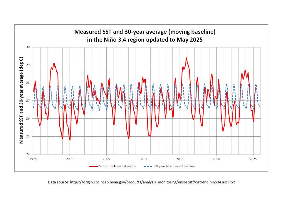
ONI is determined as the difference between the two curves shown above, averaged over rolling three month periods.
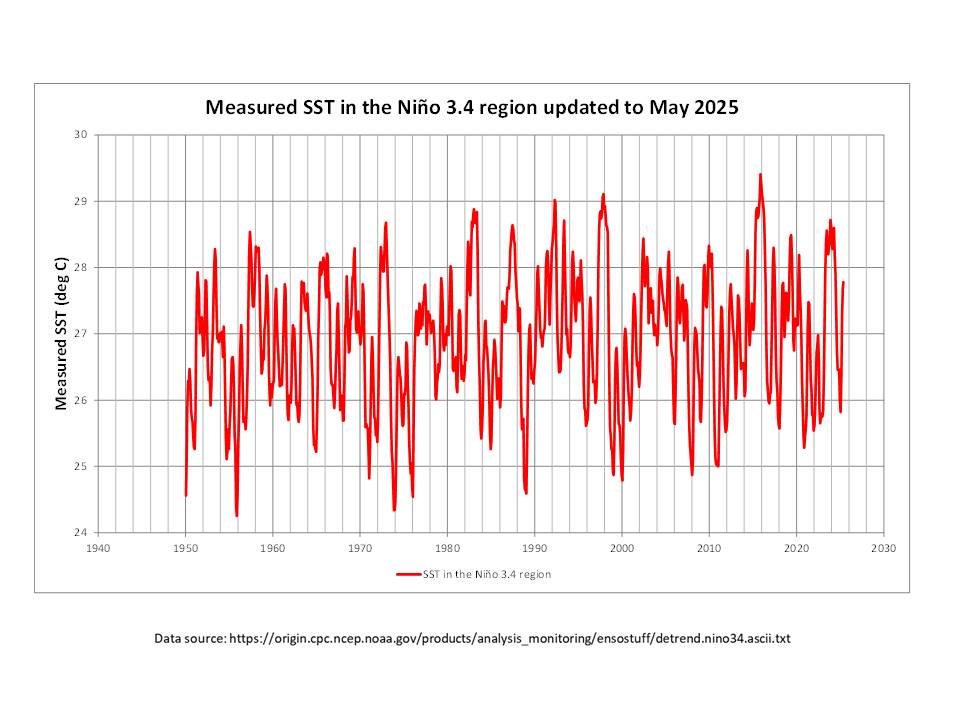
Quite often, a La Niña event (cooling relative to average) immediately precedes a significant El Niño event (warming relative to average), so this will enhance the size of the temperature increase on the UAH data. This can lead to some mis-interpretations. In 2008, for example, there was a strong (2007-2008) La Niña event which gave rise to the clear trough in the UAH data in early that year. As the temperature rebounded, there was another weak (2008-2009) event (trough), which can also be seen in mid-2009 on the UAH data, prior to a further temperature increase as the moderate 2009-2010 El Niño took hold in late-2009 (UAH data).
Also, note that the ONI values have been de-trended, forcing the classification to appear to be neutral over the longer term. However, the raw SST data used for the determination of ONI classification values do show an increasing temperature trend (particularly clear if you look at the minimum and maximum SSTs).
“First off, your designated starting times for El Niños and their indicated strengths do not at match those of the website”
That’s the same website I used. For simplicity I use the second year as the actual date of the El Niño, as there’s a lag before the full global effect. Hence the 1997-98 El Niño is marked on the graph as the year 1998, becasue that’s when you usually get the main spike.
fails to explain the rapid increases in UAH 6.1 GLAT anomalies that are seen in the monthly data starting in:
1986,
2004,
2008, and
2018.
1986-87 was a moderate El Niño, and temperatures were warming up since the cooling caused by El Chichón in 1983.
I’m not sure what you mean by 2004 – temperatures were cooling then after the previous El Niño.
Temperatures were falling rapidly in 2008, due to a strong La Niña.
And temperatures were falling in 2018, due to a week La Niña, following a very strong El Niño.
“I believe the data says different.”
Then you are going to have to do your own research on the data. To me the fact that El Niño’s usually cause temperature pikes is both well known and and obvious from any graph. Come back the next time we have a strong El Niño, and see how quick people here will be to point out the warming is caused by the El Niño, and so nothing to do with CO2.
Wow, that’s a real sleight-of-hand trick: choosing to use the second year of an officially-declared El Niño period, which is based on scientific measurements of ocean temperatures increasing above a pre-established threshold value (i.e., based on the Ocean Nino Index (ONI)). How convenient for you.
I guess there’s no reason whatsoever to suspect that ocean warming over a full 12 months before then would affect the lower atmosphere, which is it intimately thermally-connected with ocean surface water temperature via the thermodynamics of water evaporation thermal exchange? /sarc
I’m wondering how many climate scientists resort to your methodology?
Moreover, perhaps you missed it completely, but the UAH monthly data shows that that GLAT temperature anomalies, as measured by the MSUs on the multiple satellites they use, show variations of global average lower atmospheric temperature of 0.25°C or higher over periods as short as two months (for example look at the above article’s table and compare April 2024 to June 2024 “global” anomalies) . . . if that change was due predominately to changes in ocean water surface temperatures, such as associated with El Niños or La Niñas, then that falsifies any claim for there being a year-long thermal delay between the onset of an El Nino and when the atmosphere globally responds to it.
I surmise that you’ve failed to understand that I’ve been doing that very thing for many years.
And, finally, the causes of occasional periods of global warming—let alone global warming experienced over decades to centuries—are NOT binary (that is, either El Niños or atmospheric CO2 levels). I mentioned another likely cause being variations in cloud coverage, and there could be others.
Bingo!
Perhaps a safe bet with a volcano in Japan and Indonesia throwing a lot of ash into the air today.
Yep, Its been a long protracted El Nino effect, hasn’t it.
Now, about that CO2 causation? 😉
Did CO2 cause the COOLING since June 2024 ?
What’s the point of even trying to record earth’s temperature? There are 8,231,613,070 people on earth in 2025 and we all have a separate brain with our own reality, there’s no such thing as a objective external world.
Funny how so many of us all chose around the very same time to develop the subjective “reality” of the COVID-19 pandemic. I can only imagine (hah!) the surprise of those 7+ million people that subsequently died as a result of contracting the virus arising from this mass delusion. (https://www.worldometers.info/coronavirus/coronavirus-death-toll/ )
/sarc
Hypothesis testing.
What hypothesis would that be? That thermometers respond to heat?
You really haven’t any hypothesis at all, have you? You’re just trying to sound superior, instead of ignorant and gullible.
Go on, prove me wrong – that’s the way the scientific method works, isn’t it?
The new Monckton Pause extends to 25 months starting in 2023/05. The average of this pause is 0.66 C. The previous Monckton Pause started in 2014/06 and lasted 107 months and had an average of 0.21 C. That makes this pause 0.45 C higher than the previous one.
+0.155 ± 0.041 C.decade-1 k=2 is the trend from 1979/01.
+0.027 ± 0.010 C.decade-2 k=2 is the acceleration of the trend.
Rounding this to 1 significant figure means the trend has ticked up to +0.16 ± 0.04 C.decade-1 k=2.
A new record for the highest lower bound of the trend at +0.12 ± 0.04 C.decade-1 k=2 occurred on this update.
My prediction for 2025 from the 2025/03 update was 0.43 ± 0.16 C k=2.
My prediction for 2025 from the 2025/04 update was 0.47 ± 0.14 C k=2.
My prediction for 2025 from the 2025/05 update was 0.46 ± 0.11 C k=2.
My prediction for 2025 from the 2025/06 update is now 0.47 ± 0.10 C k=2.
I should note that I’m in the process of changing my workflow to R. As a result I’m using a more robust method for evaluating the trend uncertainty. It now uses a heteroscedasticity autocorrelation consistent lag-1 model via the vcovHAC function [Zeileis 2006]
And for the significant police here are the 1st and 2nd order trend coefficients and uncertainties using all available digits provided by R. Use whatever inconsistent rules you see fit to round the values to whatever you feel is less offensive for you.
0.155058405534957 ± 0.040955195786149 C.decade-1
0.027023529680222 ± 0.010063940666609 C.decade-2
A thinly disguised ad hominem attack from someone who refuses to acknowledge proper data handling techniques.
And this proves that adding CO2 to air makes it hotter?
You can’t face reality. There is no GHE. The Earth has cooled, and continues to do so. More energy leaving than arriving. I’m sure you can “calculate” the amount to 20 or 30 significant figures if you use the right coloured crayon.
Sad but true.
Ever since UAH upgraded from 6.0 to 6.1 in November of 2024 the TLT anomalies are behaving in a manner consistent with the expectation from the most recent ENSO cycle. There is that one value from 2023/09 that broke out of the 2σ envelope, but that is expected about 1/20th of the time.
The model is saying that we could still see further drops in the TLT anomalies. I don’t know if that will happen or not. Fluctuations around the 0.4 C mark are within the noise floor.
It take 5 “fudge factors” to wiggle the elephants tail. 😉
Making the assumption that CO2 causes warming, as you undoubtedly have, and then creating a fake model that shows warming by CO2…
… is the absolute anti-thesis of “science”
Here is the update for Australia, lower troposphere, from Jan 1979 to the start of July 2025.
The brown dots are global.
Both graphs are shifted 7 months to the right because of smoothing by moving average per Excel. Without smoothing, Australian trends are much harder to see.
My only comment is that June 2025 at 0.39, the last month shown, is below the average of the last 10 years of 0.42, but maybe both share the same uncertainty envelope.

Geoff S
I do understand why those who critique the standard CO2 consensus are here but what do the proponents get out of these ‘debates’? Useless point scoring in the hope someone will change their mind? Or just the excitement of irritating people?
This is a reply I got from someone on here (a science advocate). After I informed him of the antecedents of the poster he was replying to….
”I understand that Anthony, however I wouldn’t want someone to think that the rubbish he posts might be true if no-one contradicted it!”
I’m surprised no one mentioned the big drop in CFSR global temperature. While it was likely too late to affect satellite data for the month of June, it’s very likely signaling a future change.
The best guess for this change is an increase in clouds countering the decrease which occurred after the Hunga-Tonga eruption. Probably includes some overshoot. Where this settles will be a good clue as to where global temperatures are headed.
Not sure if anyone has cloud data for the period involved. That would be useful.
Dr Spencer, congratulations to you and Dr. Christy for being selected by President Trump. What a true honor and it couldn’t have happened to a more deserving group.
The Trump admin just hired 3 outspoken climate contrarians. Scientists are worried what comes next
https://www.cnn.com/2025/07/08/climate/doe-climate-contrarians-trump
I know we may disagree on some of the issues, but please consider passings these videos on to the EPA and others in Washington.
Analysis of the Hockeystick
https://app.screencast.com/nXfZcUyGR4QlR
Lawsuit Arguments
https://app.screencast.com/ZMpNTvkLD7DDJ
If 10% is correct in those videos, there are real problems, but I’m pretty sure 100% is correct. If not, readers please provide corrections.