From Dr Roy Spencer’s Global Warming Blog
by Roy W. Spencer, Ph. D.
Metop-C Satellite Added to Our Processing
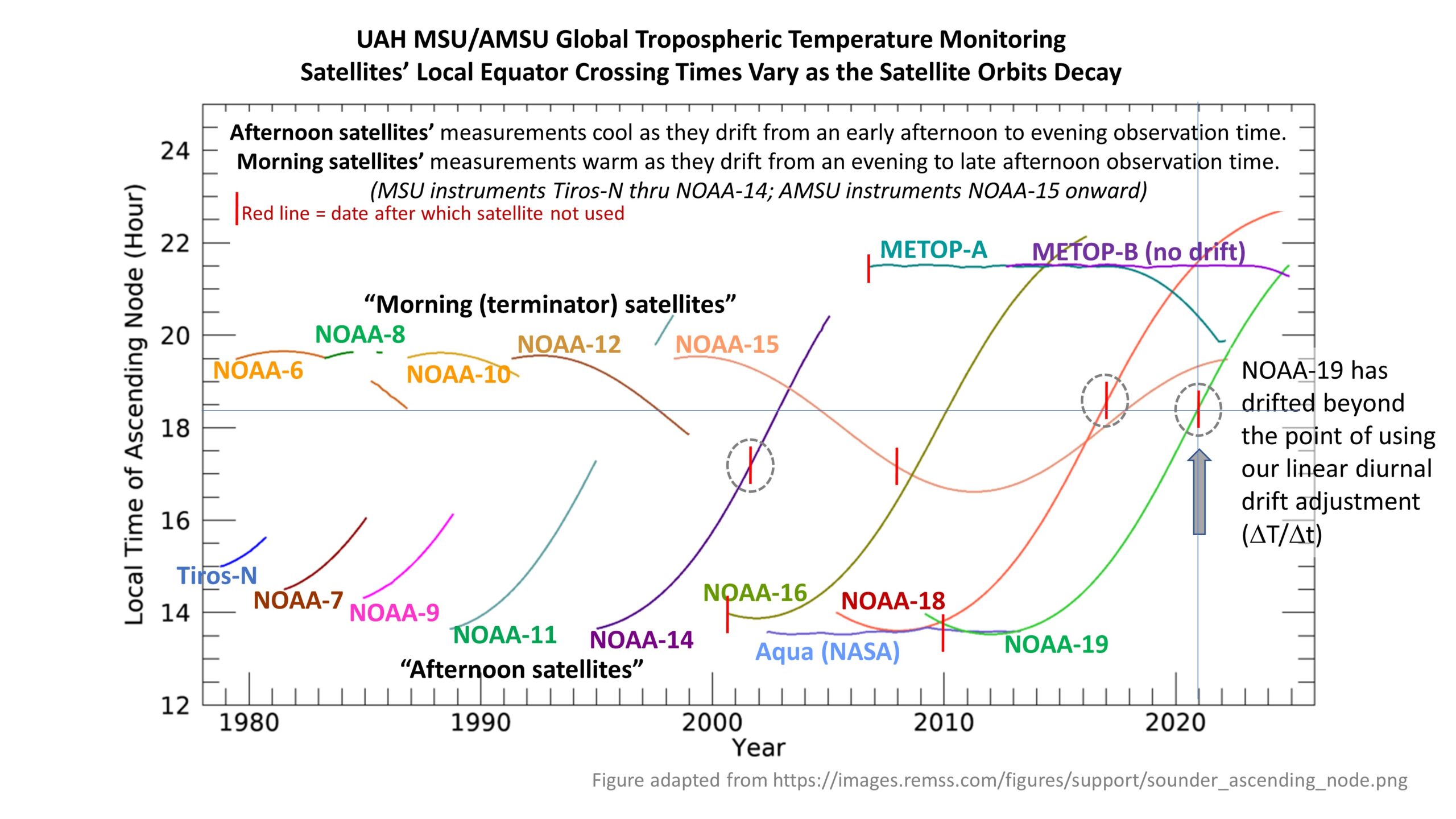
With this update, we have added Metop-C to our processing, so along with Metop-B we are back to having two satellites in the processing stream. The Metop-C data record begins in July of 2019. Like Metop-B, Metop-C was designed to use fuel to maintain its orbital altitude and inclination, so (until fuel reserves are depleted) there is no diurnal drift adjustment needed. Metop-B is beginning to show some drift in the last year or so, but it’s too little at this point to worry about any diurnal drift correction.
The Version 6.1 global average lower tropospheric temperature (LT) anomaly for November, 2024 was +0.64 deg. C departure from the 1991-2020 mean, down from the October, 2024 anomaly of +0.75 deg. C.

The Version 6.1 global area-averaged temperature trend (January 1979 through November 2024) remains at +0.15 deg/ C/decade (+0.21 C/decade over land, +0.13 C/decade over oceans).
The following table lists various regional Version 6.1 LT departures from the 30-year (1991-2020) average for the last 23 months (record highs are in red). Note the tropics have cooled by 0.72 deg. C in the last 8 months, consistent with the onset of La Nina conditions.
| YEAR | MO | GLOBE | NHEM. | SHEM. | TROPIC | USA48 | ARCTIC | AUST |
| 2023 | Jan | -0.06 | +0.07 | -0.19 | -0.41 | +0.14 | -0.10 | -0.45 |
| 2023 | Feb | +0.07 | +0.13 | +0.01 | -0.13 | +0.64 | -0.26 | +0.11 |
| 2023 | Mar | +0.18 | +0.22 | +0.14 | -0.17 | -1.36 | +0.15 | +0.58 |
| 2023 | Apr | +0.12 | +0.04 | +0.20 | -0.09 | -0.40 | +0.47 | +0.41 |
| 2023 | May | +0.28 | +0.16 | +0.41 | +0.32 | +0.37 | +0.52 | +0.10 |
| 2023 | June | +0.30 | +0.33 | +0.28 | +0.51 | -0.55 | +0.29 | +0.20 |
| 2023 | July | +0.56 | +0.59 | +0.54 | +0.83 | +0.28 | +0.79 | +1.42 |
| 2023 | Aug | +0.61 | +0.77 | +0.45 | +0.78 | +0.71 | +1.49 | +1.30 |
| 2023 | Sep | +0.80 | +0.84 | +0.76 | +0.82 | +0.25 | +1.11 | +1.17 |
| 2023 | Oct | +0.79 | +0.85 | +0.72 | +0.85 | +0.83 | +0.81 | +0.57 |
| 2023 | Nov | +0.77 | +0.87 | +0.67 | +0.87 | +0.50 | +1.08 | +0.29 |
| 2023 | Dec | +0.75 | +0.92 | +0.57 | +1.01 | +1.22 | +0.31 | +0.70 |
| 2024 | Jan | +0.80 | +1.02 | +0.58 | +1.20 | -0.19 | +0.40 | +1.12 |
| 2024 | Feb | +0.88 | +0.95 | +0.81 | +1.17 | +1.31 | +0.86 | +1.16 |
| 2024 | Mar | +0.88 | +0.96 | +0.80 | +1.26 | +0.22 | +1.05 | +1.34 |
| 2024 | Apr | +0.94 | +1.12 | +0.77 | +1.15 | +0.86 | +0.88 | +0.54 |
| 2024 | May | +0.78 | +0.77 | +0.78 | +1.20 | +0.05 | +0.22 | +0.53 |
| 2024 | June | +0.69 | +0.78 | +0.60 | +0.85 | +1.37 | +0.64 | +0.91 |
| 2024 | July | +0.74 | +0.86 | +0.62 | +0.97 | +0.44 | +0.56 | -0.06 |
| 2024 | Aug | +0.76 | +0.82 | +0.70 | +0.75 | +0.41 | +0.88 | +1.75 |
| 2024 | Sep | +0.81 | +1.04 | +0.58 | +0.82 | +1.32 | +1.48 | +0.98 |
| 2024 | Oct | +0.75 | +0.89 | +0.61 | +0.64 | +1.90 | +0.81 | +1.09 |
| 2024 | Nov | +0.64 | +0.88 | +0.41 | +0.54 | +1.12 | +0.79 | +1.00 |
The full UAH Global Temperature Report, along with the LT global gridpoint anomaly image for November, 2024, and a more detailed analysis by John Christy, should be available within the next several days here.
The monthly anomalies for various regions for the four deep layers we monitor from satellites will be available in the next several days at the following locations:
Fine, it’s going down 👍
A lot of people in 1816 would have loved today’s temperatures. Instead they died from cold and starving.
It looks a lot like the 1998 biggie. I expect it to follow the pattern and settle into a multi-year pause a few 10ths of a degree above the last long pause. All the warming has been a staircase driven by big El Niño cycles.
El Nino doesn’t explain the observed warming:
ROFLMAO.
Urban CRAP fabrication.
Is that the best you have !!
El Nino explains ALL THE WARMING in the atmospheric data.
It does not, particularly because El Ninos aren’t trending stronger:
There is simply no mechanism by which EL Nino could be driving a multi-decadal warming trend without some external energy input.
You are a moron, AJ.
Are you really DENYING the 1998, 2016/17 and 2023/24 El Nino events and the effect they had on the atmosphere… .. WOW !!
There has been external energy.. Its called the SUN.
And of course CO2 is not an external energy input, so you have kicked yourself in the rear end, yet again.
1… Please provide empirical scientific evidence of warming by atmospheric CO2.
2… Please show the evidence of CO2 warming in the UAH atmospheric data.
3… Please state the amount of CO2 warming in the last 45 year, giving measured scientific evidence for your answer.
The claim being made is that El Nino peaks keep getting warmer and warmer and warmer over time in a stepwise fashion, and that this is driving the observed warming trend. I am saying that there is no evidence that El Ninos are exhibiting a long term trend and there is no evidence that El Nino can drive the observed warming trend. I am not denying the existence of the El Nino peaks.
Are you saying the sun’s output is increasing and that this is driving the El Nino peaks to get warmer and warmer?
“I am saying that there is no evidence that El Ninos are exhibiting a long term trend and there is no evidence that El Nino can drive the observed warming trend”
See, I told you that you were a moron.
Not understanding the difference between the localised ENSO indicator and the actual energy released to the atmosphere.
STILL DENYING the effect of the three El Ninos on the atmosphere.. WOW !!!
Those three El Nino events account for ALL the warming in the UAH data.
Noted that you were totally incapable of showing any evidence of CO2 warming anywhere.
Talk about “climate deniers”, you are a prime example.
How does one characterize the amount of energy released to the atmosphere during an El Nino? Please share that analysis.
Look at the UAH atmospheric data, idiot !!
Calling someone an idiot will not change their mind, nor will it do much for the fence sitters.
“You are a moron, AJ”
What gives you the right to begin your reply with this statement? Whether you agree or disagree with another contributor, what’s so difficult about being civil?
The point AJ makes is perfectly reasonable and deserves a reasonable response. If you yourself maintain the the science isn’t settled, then it’s not settled in any sense – in terms of evidence for or against AGW. Therefore, it’s as absurd for you to claim the El Ninõ effect on warming as settled science, as it is for AJ to contend CO2 as a forcing! At least stand or fall by your own contentions.
The evidence from both satellite and land based data show a definite warming trend for several decades. At least acknowledge the possibility that CO2 might be partially the driving force. It might prove not to be so or it might become increasingly clear that there’s no other explanation outside of CO2. But crucially, science must keep minds open for further enquiry. There’s little profit in pointing the finger at mainstream climate science, claiming lack of integrity, when you engage in exactly the same tactics. The polarised attitudes do nothing at all to help clean up the mire, they just make it more filthy.
WRONG.. The UAH data shows warming ONLY at major El Nino events
Near zero trend from 1980-1997
Near zero trend from 2001-2015
Slight cooling trend from 2017/2023.4
It is basically zero trend, apart from El Nino events
If you think there is evidence of warming by atmospheric CO2 then produce the evidence.
1… Please provide empirical scientific evidence of warming by atmospheric CO2.
2… Please show the evidence of CO2 warming in the UAH atmospheric data.
3… Please state the exact amount of CO2 warming in the last 45 year, giving measured scientific evidence for your answer.
CO2 is not an energy source. It can absorb and emit radiation. But, the emission can never be greater than the absorption. Consequently, CO2, by itself, can not add heat to the system.
Until the atmosphere becomes warmer than the surface, land and ocean, the atmosphere can not add heat to the surface. That assumes the sun can not directly warm the atmosphere, but that is not manmade heat is it?
“At least acknowledge the possibility that CO2 might be partially the driving force. “
Then why was it hotter in the 30’s than today – when CO2 in the atmosphere was smaller?
Because he has proven time and time again that he is. !!
AJ is a vapid AGW apostle. Are you ???
Noted that yet again he has been totally unable to provide any proof whatsoever of CO2 warming.
Only a complete moron or a vapid AGW activist (same thing) would put forward, as evidence, surface data that he knows is both highly agenda corrupted and highly urban effected….
…especially when the whole topic is the UAH atmospheric data.
Wouldn’t you agree. !!
Something the mods here seem to be incapable of dealing with, in this particular sad individual’s case.
Yes, you are a very sad non-entity, fungal.
FYI.
Absorbed solar energy continues to increase.
So, to clarify, the argument is that absorbed shortwave radiation is driving the observed long term warming trend, not a stepwise El Nino forcing?
OMG…. this is why I call you a moron.
The sun helps charge the El Nino events.!
But you were well aware of that, weren’t you.!
Or maybe you will suggest that the SUN does provide energy to the oceans, or something daft like that.
So again…. where is your evidence of any human caused atmospheric warming in the UAH data.
So when you say that the warming is actually occurring stepwise at each El Nino, what you mean is that the warming is being driven by increased shortwave absorption, and that the warming is simply expressed at El Nino events because they are natural high temperature peaks?
Again…. where is your evidence of any human caused atmospheric warming in the UAH data.
Still a complete FAILURE !!
If you can’t understand simple concepts, not my problem
Where do you think most of the energy that is released at El Nino events comes from .. surely not CO2.. that would be dumb even for you.
I am putting aside my personal opinions about the cause of the observed warming and am exploring the theory that was proposed earlier by David. David says “All the warming has been a staircase driven by big El Niño cycles.” I’m asking what is driving the trend in the El Nino cycles. You seem to be saying it’s an increase in shortwave absorption?
Where is your evidence that “the sun helps charge the El Nino events?”
The sun’s radiation is the source of all energy (discounting geological and manmade heat) in the system. The atmosphere can be warmed directly from the sun or by radiation, conduction, convection from the surface. Either requires more absorption from the sun.
Now if one wants make an argument that all heat generated by humans from dung cooking fires to nuclear submarines to air conditioners alters the heat in the Earth’s system, feel free.
I agree that the sun is the source of all energy, but if the argument being made is that there is a long term change in shortwave absorption that is driving the long term temperature trend, and this trend is readily apparent at each El Nino highstand, that’s quite a bit different than claiming that the El Ninos themselves are providing some mode of stepwise climate forcing that is producing the observed trend.
The original poster, David, seemed to be saying the latter, and I’m not clear on where bnice stands based on their comments, or what mechanism might be proposed to allow El Nino to produce such a forcing.
If the oceans are absorbing more of the sun’s energy, then El Nino’s will obviously have higher temperatures to radiate away. An El Nino could complete at a higher temperature than the preceding one causing additional warming of the whole atmosphere.
The problem is that CO2 can’t cause the warming step but a constant low to high range of El Nino could.
So, you mean it would have to look something like this …
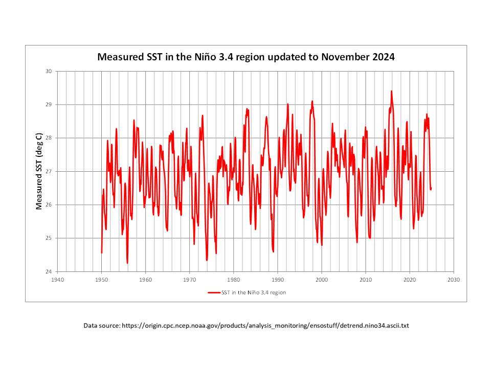
As you probably are well aware, one of the primary indicators, and classification, of El Niño/La Niña events is the Oceanic Niño Index (ONI), which is the rolling three-month average of the sea surface temperature (SST) anomaly in the Niño-3.4 region in the equatorial Pacific Ocean (5degN-5degS, 120deg-170degW). In my view, it is instructive to look at the measured SST values themselves rather than simply focussing on the ONI (anomaly) values derived from them, not least because the ONI values are de-trended.
In the plot above, the monthly SST maximum values (El Niño events) and the minimum values (La Niña events) both show a long term increase of around 1degC since 1950, while maintaining the maximum range of about 4degC.
If the warming is the result of a long term persistent forcing then the “step” appearance of the El Nino events is simply the effect of superimposing cyclic variability atop a linear trend:
So we cannot assume ipso facto that the appearance of a “stepwise” pattern in the data is indicative of any step-forcing driving the change.
But, again, as near as I can tell, bnice, and now you, are claiming that the warming is being caused by increased shortwave forcing, not by El Nino at all, which is a claim at odds with the poster I initially responded to.
Submarine volcanoes?
Earth’s declining magnetic field strength .
Please do not confuse BeNasty 2000 with data. He starts out confused. As you should know, the El Nino Nutters like BeNasty are also greenhouse effect deniers and CO2 Does Nothing Nutters. Triple Nutters.
And of course they think 99.9% of scientists have been wrong about the greenhouse effect since 1896. Based on the science degrees, science knowledge and science work experience they do not have. But they can look at a UAH chart and they see temperature spikes
What is being observed is not temperature but numbers emitted from computers after very inaccurate temperature data from an array of inaccurate measuring instruments not calibrated to a single reference instrument, are averaged, fed into a digital melting pot seething with algorithms to allow for this and that, and bubble out with exquisite accuracy far greater than that of the input data.
There are multiple independent global temperature analyses that yield consistent results, so the results are likely robust:
Statistical precision is not accuracy!
This statement is true but too general to be useful here I think. Precise results instill greater confidence than imprecise results. It is implausible to think there is a common systematic error in the various observation datasets (land, ocean, satellite), so systematic error in any form of analysis should be expected to produce disagreement among the results.
It’s hockey stick time again, kids!
Sorry, I’m not of the same mindset. While I don’t claim this is impossible, I believe there’s a better explanation. The warming over the past 30 years has been driven mainly by the +AMO phase. And, it’s recently been enhanced by the Hunga-Tonga eruption.
Over longer time periods we are seeing an influence from the millennial cycle which also led to the Minoan, Roman and Medieval warm periods.
El Niño does have shorter term effects which are countered by La Niña.
The good news is the next AMO phase change is due within the next 5 years. We should then be able to break down its contribution to recent warming.
Have a look at the UAH atmospheric data.
The ONLY warming has come at major El Nino events. !
The statement by David, that…
“ All the warming has been a staircase driven by big El Niño cycles.”
… is manifestly obvious. !
I think it may be more subtle. The AMO phase change from 1995-97 preceded the 1997-98 El Nino and had a large change in clouds associated with it. It could well be the El Nino (and multi-year La Nina events which followed) were just a coincidence but caused so much noise in the data the AMO change was hidden.
We then had the long pause with little change in temperature.
The 2015-16 El Nino also came after another cloud change from 2014-16. You’ve posted the cloud data so you can check it. Once again it could be the El Nino was just noise masking the cloud changes. The PDO also went positive in 2014 and the Bardarbunga eruption occurred.
Now we have the 2023-24 El Nino following the Hunga-Tonga eruption and yes, more cloud changes.
So, in all cases we can see cloud changes occurring which can explain the step-up in temperature after the El Nino events. To me the cloud changes are the real reason we’ve seen warming. However, they occurred before the El Nino events.
That only establishes correlation, not causation.
You and BeNasty are the head WUWT El Nino Nutters
The ENSO cycles are temperature neutral over the long run of 30 to 50 years. Since climate requires at least a 30 year average, the claim that global warming is only caused by El Ninos is claptrap. El Ninos merely caused temporary spikes in the rising trend since 1975 and La Ninas flattened the rising trend temporarily. The El Nino Nutters look at the spikes like a child looks at candy and ignore the La Ninas.
If El Ninos were the sole cause of global warming, then the global cooling period from 1940 to 1975 could not have happened. It does not take a Ph.D. to figure that out.
Assuming no big changes prior to 2023, this is the second warmest November. Ten warmest Novembers in UAH history are:
2023 0.77
2024 0.64
2019 0.42
2020 0.40
2016 0.34
2017 0.22
2015 0.21
2009 0.14
1990 0.12
2018 0.12
My projection for the year rises slightly to +0.765 ± 0.055°C, and it’s even more certain that 2024 will be the warmest on record, beating 2023 by at least 0.3°C. December would have to be -3.5°C for the record not to be beaten, so I think it’s a fairly safe bet.
Fans of meaningless trends will be delighted to know that the trend has been negative since August 2023, so a 16 month pause. How long before it reaches the magic 5 years, and the return of the monthly update?
In the mean time, the meaningless trend over the last 5 years is currently 1.1°C / decade.
How hai is a Chinaman…
不太
Not as hi as a Hunter.
“Fans of meaningless trends”
How about fans of meaningless averages?
I’d like to know where it’s been “the hottest”. There’s been none of it in my region. Oh! Wait! Maybe it’s not global, and bogus global averages give completely false impressions of what’s really happening!
“How about fans of meaningless averages?”
The meaningless average that gets published here every month, and an entire phony pause was based around.
“I’d like to know where it’s been “the hottest”.”
It’s the second warmest global average for November. I doubt many places in the northern hemisphere are “the hottest”.
It’s even more bizzare when you read that scientists use the GAT index, which includes temperatures from tropical regions, to make inferences about ice sheet feedbacks lol.
https://academic.oup.com/oocc/article/3/1/kgad008/7335889
These are all time series trends. Do you recall seeing any effort to make the trend stationary? I never see any discussions about time series analysis techniques. Just simple linear regression of variables that are not even related by any accepted functional relationship.
UAH were quick to release the gridded data this time, so here’s my map of the anomalies for November.
It’s surprising how warm it shows the UK. Ground based observations only have it slightly above the 1991 – 2020 average.
Is that Met Office data?
Yes.
https://www.metoffice.gov.uk/research/climate/maps-and-data/uk-temperature-rainfall-and-sunshine-time-series
UK sunshine
UK Sunshine for November
Correlation between sun and mean temperatures for November in the UK.
Remember, the UK is in the Northern Hemisphere.
LOL… cherry picking one month. Well done 😉
No human causation, is there.
The month we were talking about – November.
If you want to see a strong correlation between sunshine and temperature you need to look to the months with longer days, July and August show very strong correlation. But you will have to do a lot better than your usual hand waving to demonstrate that increased sunshine is the main reason for the overall warming in the UK.
This comment deleted as posted in wrong place.
What is the r^2 value for that fit? It doesn’t look very high.
For this comment?
https://wattsupwiththat.com/2024/12/03/uah-v6-1-global-temperature-update-for-november-2024-0-64-deg-c/#comment-4002745
I’m getting 0.1357. But the trend itself is quite statistically durable. There is slightly more than one chance in 100,000 that it is, in fact, flat or up.
Finally realize that R^2 is essentially use free for what you are seeking. Do the work. Download the data. Find it’s trend and the standard error of it’s trend. Note the R^2. Now detrend the data and repeat. Note that while the standard error of the trend is unchanged, the R^2 goes essentially to zero.
The standard error of the trend is only a metric for how well the line fits the data. It simply tells you nothing about the accuracy of the data and, therefore, of the accuracy of the trend line.
Only “nothing” to the extent that the data spreads increase that standard error. This is the usual goal post shift. Tell us how the uncertainty of each data point is distributed, and I’ll tell you the total standard error of their trend. Spoiler alert folks. For any credible spreads, it won’t increase much….
Error is not uncertainty.
True. Every measurement has both. But only meaningful if they have enough of them together to significantly change the evaluation under discussion. Anyone, anyone, please provide credible guesses on the errors and uncertainties in this data that could possibly do so.
How do you know the true values?
I don’t. You never do. But it’s not an all purpose way of criticizing every inconvenient evaluation you run across. Well, apparently it is for you….
Then you cannot know the magnitude of any error.
You might know this if you had any experience in real metrology, beyond Statistics Uber Alles.
AGAIN, the all purpose argument. Since every data point has error and uncertainty, only the evaluations we find convenient, should be performed using them Monckton is certainly cheering you on.
And predictably, you and the rest of your coterie continue to whine interminably about how your revealed (only to you all) truths are ignored outside of this tiny fora. I should have realized that alt.world, with it’s hard shell of circular logic, would inevitably mutate from the political sphere into health and the sciences. I’m thankful that, unlike the world outside of these disciplines, it has done so very poorly, so far.
Meaningless word salad!
I’ll try my example one more time.
You have two temperatures:
.2 +/- 0.5
.3 +/- 0.5
The possible delta’s (i.e. the slope of the connection line between the two points):
-.3 to .8 Δ = +.11
.2 to .3 Δ = .1
.7 to -.2 Δ = -.9
If you use only the stated values you get a positive slope of .1. If you use the measurement uncertainties you get slopes ranging from -.9 to +.11.
In other words you can’t even tell the direction of the slope let alone the value of the slope if you *do* consider the measurement uncertainty.
Ignoring measurement uncertainty *is* just the meme of “all measurement uncertainty is random, Gaussian, and cancels”. It’s garbage and you are trying to throw it at the wall hoping it will stick. All it does is smell up the place as it slides down the wall!
Meaningless and ignorant word salad.
He rejects the idea that uncertainty intervals are real, much less their implications.
Well, blob, you’ve just exposed your abject ignorance: metrology isn’t your long suit.
It is glaringly obvious you’ve never had to comply with ISO 17025.
NIST TN 1900 has a representative value of ±1.8°C and that should be doubled because you are subtracting two randon variables. To properly evaluate the trend line you will need to evaluate every possible combination of those values to find the variation in the trend line slope and intercept.
“NIST TN 1900 has a representative value of ±1.8°C..”
Please expand. Is this a 2 sigma distribution for every temperature measurement in the plot furnished by Bellman?
“…and that should be doubled because you are subtracting two randon variables.:
Nope. I’m evaluating the trend between 2 “random variables”.
Nope, yer just stringing random words together.
And it is bellman the weasel’s job to supply the info you seek, not Jim’s.
You can freely download this Technical Note and examine Example 2.
The ±1.8°C is the expanded experimental standard uncertainty of the mean for the monthly average value of Tmax at a station located at the NIST campus station close to I-270.
You should note that this is very similar to what NOAA states as ASOS uncertainty, ±1.0°C. Far, far above what is used when calculating anomaly only standard deviation after throwing away the inherited measurement uncertainty from the actual measurements.
How do you evaluate the trend between two random variables that have measurement uncertainty by using on the stated values?
You are just using the common climate science meme of “all measurement uncertainty is random, Gaussian, and cancels” so you can assume the stated values are 100% accurate and will generate an accurate trend line. It’s a garbage meme.
“How do you evaluate the trend between two random variables that have measurement uncertainty by using on the stated values?”
Per this absurdism, you never can. In any case, anywhere. But thankfully, above ground, people use common sense. They judge the upper bounds of credible error and uncertainty ranges for the data, and use them to bound possible resultant uncertainties for evaluative results. If they don’t significantly change those results, they go with them, and refine them as required.
For the 2 sigma 1.8 degC range that you referenced for temperature, and for Bellman’s last example, the good news for you is that the chance of the trend being wrong increased – as it should. The bad news is that it increased from slightly less than 1 in 100000 to 1 in 100. So, qualitatively, Bellman went from being probably right to being – er – probably right.
But thankfully, above ground, people use common sense. They judge the upper bounds of credible error and uncertainty ranges for the data,
Give one example of a climatologist providing real uncertainty “judgements”, blob. Just one.
I dare you.
If the difference between adjacent points can be down because of measurement uncertainty then the slope of the line between them will be down. *YOU* eliminate that possibility by just assuming no measurement uncertainty and the stated values are 100% accurate!
This is nothing more than one more invacation of the garbage climste science meme that “all measurement uncertainty is random, Gaussian. and cancels”. If the temp change is 0.2 +\- 0.5 then you simply don’t know if tge trend is up or down. So you and climate science just WISH away the +\~ 0.5!
Nope. I never claimed any of that.
“If the temp change is 0.2 +\- 0.5 then you simply don’t know if the trend is up or down.”
You never “know”, in any case. But you do “know” that a trend of 0.2, with a standard error of 1.0, still has a 58% chance of being positive. Bellman’s trend was for an expected value of -0.046 deg/unit change in solar intensity, with a standard error of 0.011 deg/unit change in solar intensity. Do the work and you’ll get the same chance of it, in fact, being positive as me.
Your all purpose diss is that the data has “errors” and “uncertainties”. AGAIN, provide any credible estimate of how much, and we can find out if it changes things enough to matter.
Technical words of which you have no understanding, thus you try to paper over your ignorance of same with yet another word salad (YAWS).
The 0.2 is *NOT* the slope of the trend line. It is the difference between two adjacent data points. Meaning the difference could be positive or negative. We’ve been down this road before. If *all* the differences between adjacent are negative then the slope *has* to be negative. You immediately eliminate that possibility by using the “all measurement uncertainty is random, Gaussian, and cancels” meme so you can concentrate on the stated value alone.
“There is slightly more than one chance in 100,000 that it is, in fact, flat or up.”
If that is so then the trend also has slightly less than 99,999 chances in 100,000 (i.e. it’s almost certain) that it is, in fact, DOWN!
Is that what you intended to suggest?
Yes, six is indeed a half dozen…
What are you talking about, bob? I don’t have time to play mind-games.
Many have wondered the same…
I’ll check when I get back, but it’s pretty low for all months apart from July and August.
It’s better if you look at annual data, but I think that hides a lot of the details. I keep looking at the data, but don’t think I can draw much of a conclusion. Quite possibly some UK warming is caused by increased sunshin, but it can’t explain all or most of it. And that still leaves the question of why sunshine has been increasing over the last 50 years.
R^2 for November is 0.14.
As I said, only the summer months have a reasonably strong R^2.
The months with the shortest days tend to have negative correlation. They also show the strongest slope, which may just be because there is less variation in the number of hours in the month.
You just explained one reason why Tavg on a global basis is a joke. One half of the globe has winter and short days while the other half has summer and long days. Do you really think that combining opposites gives a statistical significant answer? You mention “hiding”. Guess what?
They have all been trained to think solely in terms of GATavg, and cannot escape this trap.
“You just explained one reason why Tavg on a global basis is a joke.”
You need to explain where you think I said any such thing. Did you ever mention to Monckton that his pause was a joke based on the UAH global mean?
“One half of the globe has winter and short days while the other half has summer and long days.”
So you accept the worlds round at least. Though you don’t seem to think that the tropics exist.
“Do you really think that combining opposites gives a statistical significant answer?”
The anomalies are not “opposites”. Look at the UAH data. Currently both hemispheres have positive anomalies, and have had them for the past year or so. As to statistical significance, you will have to explain what your hypothesis is. If the hypothesis is that global anomalies have increased over the last 40+ years, then I think we can say the results using the global average are statistically significant.
“You mention “hiding”. Guess what?”
Why do you always have to speak in riddles. Where did I mention “hiding”? What was the context? What do you want me to guess?
The anomalies inherit the variances of the absolutes. Meaning the anomalies in each hemisphere have different variances. You *have* to add them using proper weighting – which climate science never does. It just averages the anomalies while ignoring the variances – just like they always ignore measurement uncertainties.
He will never admit this is true.
You really need to figure out what it is you are asking and then explain it clearly. And tell it to Dr Spencer rather than me.
I tried to do what I thought you were after a couple of months ago, but you just blew it away. But again, here’s the UAH data expressed in terms of local deviation from the 1991-2020 base period. It’s an interesting approach as it shows where a particular anomaly is unusually high or low for that location and time of year.
And I can produce a global average based on that metric.
The standard beelman weasel.
Thanks showing everyone it is extra sunshine, and NOT CO2 causing the warming.
Doing well 🙂
Correlation does not imply causation. But obviously it’s rain that is making the UK warmer.
Still absolutely ZERO EVIDENCE of any human causation
You are doing well, Bellboy !!
But he’s got his 12-gauge shotgun pointed at paper targets.
Yep, I reckon that’s wrong for the UK. I think the bulge of warmth across the Atlantic has been extended too far east. The UK just hasn’t been that warm in November.
Does that tell you something about the difference in measurement techniques being used? Perhaps they are not comparable at all!
And here’s the average of the last 12 months. (Note, I’ve changed the temperature scale to allow for more detail.)
That the effect of the 2023 El Nino event has been hanging around , hasn’t it.
No evidence of any human causation though, is there.
And in relation to the discussion of the 17 month pause in Australia discussed below, here are what the trends across the globe are like since July 2023.
Note, the scale is running from -20°C / decade to +20°C / decade, which should give some indication of why I think it’s meaningless.
Yep, look at the tropical area cooling down, exactly as expected.
A slower decline from the 2023 El Nino transient because of the extra WV in the stratosphere..
Absolutely ZERO EVIDENCE of any human causation. in the whole of the UAH data.
Lets run Sept, Oct Nov together.
You can clearly see the tropics is finally clearing from the solid yellow it has been since the start of the 2023 El Nino.
I actually expected it to last a bit longer.
PS.. I hate how WordPress blurs images, just click on it to get an unblurred one
“You can clearly see the tropics is finally clearing from the solid yellow it has been since the start of the 2023 El Nino.”
As this article points out, the Tropics have cooled by 0.72°C since March. I’m not sure why that should be a surprise, given the end of the El Niño. In 1998 the Tropics cooled by 1.04°C over the same period.
Here’s the graph again, using the correct version of the data.
March – November 2024
You can see the El Nino effect starting to subside, just as I said.
Well done !
Evidence of human causation NONE. !
Still waiting for you to admit that the 2023/24 El Nino event was NOT ANTHROPOGENIC in any way shape or form.
“Well done !”
Thanks. But I can’t claim credit for the theory that El Niño effects subside. If they didn’t El Niños would cause permanent warming which is absurd.
“Still waiting for you to admit that the 2023/24 El Nino event was NOT ANTHROPOGENIC in any way shape or form.”
Why should I admit something I’ve never disagreed with. I’ve never claimed this or any El Niño was caused by Humans.
Thank you for agreeing that ALL the warming in the UAH atmospheric data in NON-ANTHROPOGENIC.
Perhaps there is hope for you. !
Yes, the El Nino effect is finally winding down… slower than usual.
At least now you are admitting this is all just part of the El Nino event.
You really like your pathetic strawmen arguments, don’t you. Nobody has ever suggested that El Niños do not cause a warming spike, and hence temperatures cool down after the El Niño ends.
It’s something I and others keep pointing out when ever people keep claiming spurious pauses caused by El Niño spikes.
The question this time is whether this particular spike can be explained entirely by this particular El Niño, and I’ve always said we probably won’t know that with any clarity for some time.
Again, Thanks for admitting that there is absolutely no sign of any human caused warming in the UAH data.
No room for any imaginary CO2 warming.
And no, you have it totally bas-ackwards… El Ninos break the zero trend periods.
They start after an El Nino spike/step, and continue until the next El Nino.
No human causation anywhere… as you continue to emphasise.
Have they released the latest adjustment to their ‘pristine’ data yet?
dolt !!
““Fans of meaningless trends””
That’d be YOU !!
“that the trend has been negative since August 2023, so a 16 month pause.”
Yep a slow escape of the 2023 El Nino energy, actually peaked in April 2024.
Why is the trend so meaningless. Please explain! If the trend becomes downward over time, would you still contend that it would be “meaningless”?
Bellboy is what we call a “trend monkey”
He thinks linear trends can be applied to everything, and loves using step changes like at El Nino events, to create linear trends.
Looks like the 2023 El Nino energy is finally dissipating… slowly.
bnice2000 is what we call a “liar”. He claims I think linear trends can be applied to everything, despite the fact I specifically called them meaningless.
I’ve constantly criticized the use of linear trends applied to make spurious points, including those used by Monckton and others to claim pauses, whilst ignoring the uncertainty in the short term trend, and the cherry-picking nature of the choice of start date. I’ve made the same points about bnice2000 claims of “step changes”. Again the result of selecting arbitrary short term trends, and ignoring the uncertainty and ENSO conditions.
Poor bellboy.. writes a post highlighting his ignorance.. Very funny !
He knows the only way he can show a positive linear trend is to use the El Nino spike/steps, which he invariably does.
LYING to himself, fooling no-one but himself… and too dumb to realise it.
Selected short periods that are El Nino.. or can’t you tell when the El Ninos are, little child. !!
No cherry-picking needed! They are where they are.
And they have step changes that are patently obvious to anyone but a blind monkey !
And the bell-child is always running away when asked to produce evidence of human causation.
Monckton calculation is not spurious in the least. It asks a set question, then does a mathematical calculation to answer that question.
For one thing it is a time series. Analyzing time series has requirements that are not met by simple linear regressions.
Another is that in simple terms the global temperature follows a distribution with the max at the tropics and the tails at the poles. Think a normal distribution. To properly describe the GAT ( Global Average Temperature) one should also include a variance description.
1 mK!
HAHAHAHAHAHAHAHAHAHAHAHAHAHAH
I thought that would trigger you. As you clearly don’t understand what the ± 0.055 means, and are incapable of understanding why it might be better to avoid premature rounding, and as you are incapable of figuring out how to round numbers in your head – then just for you:
Dork. Both you and Spencer need to learn significant digit rules.
Oh, you know better than Roy Spencer now… Clever boy.
Poster child for WUWT.
All you’ve done here is expose your abject ignorance of significant digit rules.
Good job.
Have you ever calculated what irradiance change is necessary to contribute a temperature change of 0.001K? Can the detectors on the satellites accurately detect that small amount of change.
Tell us what the ΔW/m² is for a change from 276.000K to 276.001K!
Then tell us what the specification of the satellites have for detecting changes.
If you want to criticize Dr Spencer, do it to his face, rather than through me. My indifference to the “rules” of significant figures is my own heresy.
Thanks for admitting you only post to WUWT to torque people up.
“He’s a troll, Tim” — Pat Frank
Truer words…
He is obviously aware that the 2023 El Nino event energy has had trouble escaping.
And still no proof of a CO2 causation.
+0.765 ± 0.055°C translates to 273.915 K ± 0.02% as a relative uncertainty!
Absurdly absurd.
He doesn’t know the difference between precision and accuracy.
Nor error and uncertainty.
We’ll be able to see how absurd it is once we have December’s figure.
And in case you are not getting this, the projection is for what the UAH annual average will be. I make no claims to the accuracy of that data. The simple fact is that with just one month to go the likelihood of the annual average changing by much is small.
December only needs to be between 0.11 and 0.90 for the annual average to be within that ±0.02% range.
Right because who cares about data accuracy, right? It’s only a trivial detail!
/sarc
/plonk/
He doesn’t even realize he’s undermining himself 💀.
There are seasonal differences in instrument functionality that need to be weighed accordingly.
Religious faith is a great thing, isn’t it?
When the significant figures suggest only a centiKelvin is justified.
Exactly.
I am not interested in warming records. Right now I am battling sub-freezing COLD.
Multiple downvoting of a presentation of the actual data from the regular monthly posting on this site!
Actual data
Yes and at least 22 people downvoted it!
Hope your safe bets are better than the Iowa polling “expert” who had Harris beating Trump by 3 points.
ps – I’ve never had to rely on any models to tell me that there is no such thing as a “safe bet” in anything.
Particularly so where “chaos” is the dominant influence.
Correction –
there is one “safe bet”.
Life – nobody is coming out of this alive.
If you want to put some money on 2024 being colder than 2023 according to UAH, then be my guest. Just say what you think the odds are.
Betting on any of nature’s vagaries is how species become extinct.
Like, for example – betting that humanity will have a viable replacement for modern life-sustaining fossil fuels such as coal, oil and gas before they become rare commodities.
Jeez, who would be that stupid?
Edit –
betting that humanity
will haveHAS a viable replacement(is it beer o’clock yet?)
“(is it beer o’clock yet?)”
Always ! Somewhere.
Just contact a friend in the right time zone, via chat.
And have a beer with them. 🙂
I don’t know why, but that reminded me of a message on the side of a 12-pack of Yuengling beer:
“Please Recycle
Save our Planet
It’s the only one with Beer.”
😎
at last!- a rational reason for recycling.
You are obviously well aware that the El Nino effect has been hanging about for most of 2024, as opposed to only 6 months of 2023.
That means you are obviously well aware that this is NOT anthropogenic.
Can you bring yourself to say it. 😉
“Can you bring yourself to say it.”
Still waiting ! 😉
Do you just pull these random insults out of your fundament? Nothing you said has the slightest relevance to my comment, which was about how safe a bet it is that UAH will say 2024 was the warmest year in record. The reason why it’s the warmest is irrelevant to that bet.
Where was the insult?
Asking you to tell the truth ? sorry you think that is an insult. 😉
Come on.. have the guts to say it. or keep squirming.
You are making a victim of yourself.
Repeat after me…
“The 2023/24 El Nino has no human causation, and is totally Non-Anthropogenic.”
Just like the 1998, and 2016/17 El Ninos.
That is why there is no sign of any human caused warming in the UAH data.
I know its hard for you to admit the facts, but at least try !
And still totally natural because of the “hanging in there” effect of the 2023 El Nino + HT WV
Absolutely zero evidence that this is related to human caused “Klimate Khange with a trade mark”.
anomolies are not temperature records … especially when the underlying data is “massaged/tortured” until it yields what you want … and thats not even dealing with UHI and horrid thermometer siting issues … you don’t have ANY good, fit for purpose data to make ANY projections with …
“thats not even dealing with UHI and horrid thermometer siting issues”
Haven’t you worked out yet that this thread is about satellite data?
So what?
Everyone noticed how you conveniently snipped his main point about your precious anomalies.
I’ve lived longer, literally, than the satellite records.
Keep the records honest to pass on and in a hundred or two hundred years they will be useful for a real look at real “Global” temperature trends.
The global average temp is not even a metric for CLIMATE.
A 1C change from -20C to -19C somewhere on the globe does *NOT* change the climate at all, either locally, regionally, or globally. Same for a change from 70F to 71F.
It can’t even tell you if it is getting *warmer* since warmth is determined by the heat content, i.e. the enthalpy.
Yet climate science enthusiastically refuses to convert from using temperature as a metric to using enthalpy.
Why do you suppose that is?
O/T
On the Grenadian island of Carriacou, even the dead are now climate victims – The Guardian.
Will ghosts, poltergeists, demons etc rise up in anger?
Poor victims. !!
It shows just few feet up from the shore it is already a metre above sea level. They’re gonna be aaaaaalright.
The nearest longish-term tide data I could find shows 2.16mm/year…. SCARY !!
And of course the beach will build itself up as the sea rises.
Send in the ruler monkeys…
Looking at the current crop of Western “leaders”, I am ready to swap out for monkey rulers.
And the Earth just keeps on turning.
Yet another adjustment from UAH.
Are they back to being ‘pristine’ all over again?
Navel gazing can be fun – if you’re that way inclined.
-3
And three people are.
That “adjustment” is called “doing science the careful and proper way” . . . as in monitoring one’s data gathering instruments to minimize error sources, both known (as in diurnal drift from a satellite that has run out of propellant for maintenance of its orbital ephemeris) and spurious/random.
But it looks like you are unaware of such a concept, despite it being specifically mentioned in the above article.
I agree. I’m just pointing out that UAH cannot be considered to be pristine, or ‘gold standard’, etc as is often proclaimed here. It’s flawed and needs constant revision and adjustment, like all the other data producers.
It’s funny that when surface temperature data producers like GISS and NOAA make similar adjustments, even describing their reasons and methods in peer reviewed papers, they are often accused here of fraud.
It does get a bit suspicious when a plot of their adjustments almost match a plot of their surface temperature anomalies.
As soon as you “adjust” (that is – “tamper”) with recorded observations, you no longer have “data”, you have “constructs“.
And if you need to use your constructs to prosecute a particular case, full disclosure of your method and treatment of inputs should explain upfront that your constructs are your version of recorded observations, and as such, your conclusions are better described as “opinion”.
And as has accurately been observed for aeons, opinions are like arses – everybody has one.
Hmmmm . . . just wondering if that applies to things like rounding off “recorded observations” to the number of mathematically-supportable significant digits or to calculating an average of a given number of recorded data values?
And if an instrument circuit failure causes zero output, but the parallel data recording system keeps recording “0.0000, 0.0000, 0.000, . . .” for tens to hundreds of times, must one include those “recorded observations” for fear of elsewise being accused of constructing/adjusting/tampering with “data”?
Data rounding and flagging poor or nonexistent data is nowhere close to the fraudulent Fake Data practices of climastrology.
One of these is standard data handling techniques, the other is fraud.
The critical deficiencies of climate “data” –
Bingo.
That may well be true, but fraud wasn’t mentioned by Mr. in his post, nor in my reply to him.
Your “questions”:
Nope.
And if an instrument circuit failure causes zero output, but the parallel data recording system keeps recording “0.0000, 0.0000, 0.000, . . .” for tens to hundreds of times, must one include those “recorded observations” for fear of elsewise being accused of constructing/adjusting/tampering with “data”?
Nope.
Both of these are standard data handling techniques.
His statement:
…is exactly right, it is fraud.
What about applying a calibration curve (adjustment) to recorded observations (i.e., recorded data). I do believe NIST does that all the time with their laboratory measurements of experiment data.
Personally, I wouldn’t accuse NIST of tampering with or “constructing” data because they use this process. But I guess that’s just me.
So, please, carry on.
Where do you get “calibration curves” for historic air temperature data?
Thanks for admitting you are just another Fake Data fraudster.
You typically use calibration curves for electronic temperature measurement instruments, typically a resistance temperature device (RTD) such as a platinum resistance thermometer (PRT) or a disimilar-metals voltage-generating device such as a thermocouple. The calibration curve is needed to convert the easily electronically-measured parameter, for example resistance in a PRT, into an equivalent temperature because there is not an exact linear relationship between the two, as show in the attached graph excerpted from https://blog.beamex.com/pt100-temperature-sensor .
To the best of my knowledge there is no instrument that does not use an intermediary (such expansion of liquids in glass thermometers, or radiometers in pyrometers, or electronic devices such as RTDs and thermocouples, or IR photodetectors in thermal imaging systems) to “measure” the temperature of a given object or medium. All have non-linearities that require calibration curves to obtain highly accurate conversion of the physically-measured parameter into an equivalent temperature.
You only use calibration curves if you want the highest levels of accurate temperature “measurements”. You may not know this, but “historic air temperature data” was NEVER required to be highly accurate! Usually, +/- 0.5 deg-F was good enough.
The have been numerous WUWT articles that discuss the various inaccuracies associated with “historical”, archived temperature data.
Now, you were saying something about admitting something . . .
Nice rant. Converting a sensor output signal to temperature has NOTHING to do with the abuse to which climatology subjects air temperature data. They (and you) believe they can reduce “error” years after-the-fact.
First you wanted to question the use of calibration curves as they appear to be missing from “historic air temperature data” . . . but now you choose to divert to conversation over to “abuse” of data without even defining what you mean by that?
Why am I not surprised?
BTW, I’m glad to have provided a rant that pleased you.
BTW^2, I know for a fact that photo-manipulation programs (e.g., Photoshop) can correct errors in existing photos (e.g., scratches, printing blemishes, faded contrast, washed-out colors, astigmatism) years after they were taken. I have no problem with that. I know that similar after-the-fact-error-correction processes are used across multiple science disciplines.
They do not “correct” errors. They estimate a value from the surrounding information. There is an uncertainty associated with doing this.
Many moons ago I did photo retouching using Photoshop. You could magnify down to the pixel level and replace with an estimated RGB value. Invariably, at a macro level, you see that the surrounding pixels then needed shading to make a smooth transition.
This is why stations are “retouched” multiple times as the algorithms begin to shade further and further abroad to make smooth transitions.
For physical measurements, each and every change should be documented in a database with an explanation of why.
In business, this climate science practice will get you hung by your thumbs and flayed by lawyers. Why does climate science allow it?
And it is ever so easy to lose information in a photograph with the various enhancement algorithms.
Here’s a nickel, kid, go buy yourself a clue.
That’s all you got?
It’s all you deserve, dork.
Care to address the message and not the messenger?
ROTFLMAO.
Dork.
/plonk/
“a resistance temperature device (RTD) such as a platinum resistance thermometer (PRT) or a disimilar-metals voltage-generating device such as a thermocouple.”
You’ve been down this rat-hole before. Even PRT sensors have given calibration drift factors based on long term heating from current flow. The calibration curve developed before the sensor is installed in the field will *NOT* be correct after a period of time suffering from operating heat.
The is absolutely no reason that a time-of-use-dependent calibration curve for a PRT cannot be generated and used to offset “operating heat”, assuming such is even significant.
Duh.
Have at it. Be sure to publish your results.
I am constantly amazed at how little those supporting CAGW know about the real world.
In the other comments section this guy was trying to claim that paper has never been used to insulate wire cabling.
paper insulated cabling was a major repair issue in the telephone system, especially in residential areas. It was a never ending battle to keep the cables from getting wet and noisy. In the 70’s there were nitrogen bottles hooked into many cable runs in my neighborhood to keep a positive pressure which kept the water from getting in.
My guess is that this guy has never wired a house with old Romax cale where the wires were paper insulated.
Yep!
You guessed wrong . . . look to the words in the postings to which you might be referring. BTW, you refer to wiring for telephone “systems”, whereas the real issue is that related to electric power wiring in homes.
I grew up in a 1880’s era Victorian house that—guess what—had uninsulated wires stung between ceramic standoffs in its attic. That pre-dated Romax cables!
Flat out made up and positively FALSE!
Malarky! It’s called “manufacturing tolerances”.
For “a” PRT, as in a single one, how do you generate a time-dependent heat drift curve when you don’t even know the environment it will be installed in? It’s the *heat* that is important, a PRT in a an Arizona desert station will see a higher heat drift total than one in Nome, AK.
He doesn’t know about the standard RTD calibration curves either.
The calibration curve for PRTs (of a given type/brand) do NOT vary from one unit to the next . . . they have a calibration curve that is based on operating temperature versus time. It is inherently based on the exact materials (alloys) of construction, NOT the manufacturing date or lot number or the location where such PRT may be used!
Now, you were saying something about malarky . . .
From Fluke:
“Calibration is performed by measurement of the resistance of the unit under test (UUT) while it is exposed to a temperature. Fundamentally, four instruments are required as follows:
Each individual sensor requires calibration which generates a calibration curve. There is *NOT* one calibration curve for a given type.
From Cole-Parmer:
Calibration Procedures
Characterization
Characterization is the method that is most often used for medium to high accuracy PRT calibration. With this method, a new resistance vs. temperature relationship is determined anew with each calibration. Generally, with this type of calibration, new calibration coefficients and a calibration table are provided as a product of the calibration. There are five basic steps to perform as listed below:
Did you *really* think that manufacturing runs at different times won’t affect the calibration curve of individual PRT’s?
Read the GUM Section D.3. 3. If one has a calibration curve for the device, the realized value is corrected at the time of measurement. The correction value should be recorded with the measurement for future reference.
Read this site and carefully examine the simple uncertainty budget that is shown.
https://www.muelaner.com/uncertainty-budget/
Where do you find a calibration chart it uncertainty budget for each station location in the past?
Read this part of the GUM:
F.1.1 Randomness and repeated observations
See if you determine why NIST TN 1900 calculated uncertainty in the fashion they did based on this section.
Wherever/whenever did I state, or even imply, that applying calibration curves reduced measurement uncertainties to zero?
I see you are having loads of fun with lame semantic games.
Facts matter.
If that isn’t your implication of the usefulness of a calibration curve then why mention? What’s your point? My guess is that you don’t have one!
That’s a very poor guess on your part.
“laboratory measurements”
The operative words in your statement. Field measurements, including satellite measurements, are not done in a lab!
it is *exactly* what measurement uncertainty is meant to convey! You don’t change the data, you change the measurement uncertainty interval to account for possible inaccuracy.
Absolutely, but climatology rewrites rules then claims the ability to remove “errors” after-the-fact.
No.
Obvious crap is just obvious crap.
No “adjustments” required.
Just toss it out altogether.
I see, said the blind man.
This (half) blind man can still make out crap when it appears in front of him.
And he knows what to do with it.
Just as the gorillas in the zoos do – chuck it at the imbeciles fixated by it.
Rounding recorded observations is not a thing. Manipulating calculations in a fashion that is accepted globally by the use of significant digits rules is done to preserve the information that is available from measurements.
From: http://www.astro.yale.edu/astro120/SigFig.pdf
In other words there is a reason for significant digits rules. If you wish to disagree with them, then show your argument.
.
As to rounding averages to the resolution of the least precise measurements being averaged, the same concept applies. Simple arithmetic CAN NOT add information to measurements. A simple example is 2 in²/3 in. Where does one decide to stop showing how accurately the result can be displayed? Sig fig rules indicate the proper result is 0.7 in. Would you show 0.66666667?
Why is it so hard for climate science to understand basics like these?
WOW, really? Who knew???
/sarc
Well, you better point that out to Roy Spencer and Co at UAH. They are currently on their version 6.1.1 of the various recorded observations.
I guess you view UAH as a ‘construct’?
The same old tired, trite propaganda of the Fake Data Mannipulators.
A reliable construct.
… compared to the GISS et al junk built on lies, data tampering, fakery and urban warming.
No GISS et al make adjustments on past data on a whim using fake statistical homogenisation.
Which is NOT science.
But you are incapable of understanding the difference.
This monkey is always trying to stir the pot.
At some point, the adjustments should cease. But GISS and NOAA continually adjust the adjustments as well.
Remember, the canvas bucket 30 second evaporation correction of ship measured ocean temperature can only evaporate once.
Lol
Don’t confuse fungal with facts.
Seems to have made very little difference to the previous version. Having two satellites should be a big improvement over one.
The fact there is so little change shows they were doing a pretty good job with just one.
Right, but they both support a statistically significant global warming trend.
The extent of the change isn’t really my point; in fact I applaud them for making these adjustments.
My point is that no global temperature data set, by their very nature, can be considered ‘pristine’ or ‘gold standard’.
UAH may have a slower warming trend than all the others; but it’s still a statistically significant warming trend.
Global average temperature should never decrease if the well mixed atmospheric CO2 is driving the warming.
After all, the global average mass of atmospheric CO2 is always increasing since 1850.
The thing is that the extended El Nino event of 2023/24 had absolutely nothing to do with CO2, human or otherwise.
“Global average temperature should never decrease if the well mixed atmospheric CO2 is driving the warming.”
That would be true if CO2 was the only factor effecting temperature – but nobody suggests that.
There is no evidence CO2 a “factor” at all.
You have continued to prove that. !
Not disputing that. Just pointing out that this is a further adjustment to the UAH satellite data that many here seem to think is carved in solid rock.
It’s as fallible and moveable as all the other sources, surface or satellite.
They all paint the same general picture of continued warming, though.
No they don’t.
The satellite data shows warming only at major El Nino events.
You have yet to show us any evidence of warming by CO2 or any other human causation in the satellite data.
A total and continual FAILURE.
And no, it is far more robust that anything coming from randomly spaced junk and fabricated urban surface stations.
Very tiny adjustment in the method of extracting NEW data, due to the use of an extra satellite.
This should actually IMPROVED the measurements.
They will never be “pristine”, but but far the most consistent and reliable we have available.
This cannot be said about the highly corrupted and constantly past-changing of often-fake surface data.
You’ve missed the point, my angry wee mate.
It’s fine to make adjustments that improve your data.
It’s not fine to criticise one group for doing it whilst ignoring the other that does exactly the same thing.
For years here WUWT complained about the NOAA and GISS adjustments to the surface temperature data, even though their methods were clearly set out in peer reviewed journals.
The satellite UAH data was held up as the ‘gold standard’; yet UAH made some of the biggest trend changes of all the global temperature data sets and continues to make change after change.
“…the most consistent and reliable we have available…”
I hardly think so.
Lol
You missed the point, that is because you have zero comprehension of the difference between scientific re-calibrations, and deliberate agenda-drive fakery and mal-adjustments and urban crappymess.
Yes, you hardly think !!.. you have shown you are basically incapable of it.
Zero is exactly the correct amount. None, zip, nada, nil.
Polar bears won’t know what ice is in 2027-
Arctic could be ice free by 2027 in ‘ominous milestone’ for the planet
assuming they’re not all extinct by Xmas of course.
For the past decade the concept of “ice free” had the definition of less than 1 m sq. km. or (1 Wadhams). See: Peter Wadhams, who predicted an “ice free” Arctic Ocean by 2020 – in 2014. Similar predictive failures have been made by others.
Moving the goalposts – has Professor Wadhams Explained His Now Changed ‘ice-free’ Arctic Prediction? – Watts Up With That?
That’s a ludicrous definition. Ice free should mean no ice, not a MILLION sq. km.
Arctic sea ice will start to increase. It’s near its 30-35 year sea ice low phase (currently at 30). This means the sea ice will soon start increasing.
Are we doomed yet? 🙄
The UK is…
Yes. I predict that you’ll pay more to solve non existent problems for the rest of your life.
For all the Hunga-Tonga-eruption-explains-the-spike-in-UAH-GLAT-trending-despite-the-18-month-delay-in-its-occurrance proponents out there, please note the following consistently warmer temperatures in northern hemisphere LAT compared to southern hemisphere LAT based on the UAH data provided in the above article:
Aug 2024 — 0.12 C warmer
Sept 2024 — 0.46 C warmer
Oct 2024 — 0.28 C warmer
Nov 2024 — 0.47 C warmer
(note: not that I personally believe such numbers are accurate to two decimal places)
Hmmm . . . this happening despite the facts that (a) the Hunga-Tonga volcano is located at -20.5 degrees latitude, that is, in the Southern hemisphere, (b) the most significant one of the Hunga-Tonga undersea volcano eruptions took place on January 15, 2022, and (c) the average solar radiation intensity in Earth’s northern hemisphere is declining while is it simultaneously increasing in the southern hemisphere during the months of August through November.
It appears then that HT-injected water vapor “decided” to race up to the northern hemisphere’s stratosphere to cause excessive warming there, but not hang around in the southern hemisphere’s stratosphere to cause even the slightest additional warming there. And all the while, atmospheric physicists assured us the water vapor would be uniformly distributed across Earth’s global stratosphere certainly within one year from time of the eruption! /SARC
Not to mention the purported increase in water vapor was 0.1%.
Yeah, I am so sick of the Hunga-Tongan Climatist Cult that I want to throw my computer out of the window. These people have invalidated everything they ever said in critique of the “greenhouse effect.” It seems they are perfectly willing to assign climate blame to minuscule changes in the level of trace gasses, as long as the gas isn’t CO2.
All you need to do is dig down into the details a little deeper and it all makes sense. There are few people who deny certain gases have unique radiative properties, aka greenhouse gases. I think most of them also accept that water vapor is the strongest greenhouse gas.
When you look much closer at the science you find out CO2 does have a warming effect which fades away as it reaches low atmospheric saturation. Since this has always been the case on planet Earth, it is not possible for CO2 to cause any warming.
Water vapor has also reached low atmosphere saturation, but it is not a well mixed gas. As a result, it can and does have significant effects higher in the atmosphere.
It actually moved to both the NH and SH high latitudes and is clearing over the tropics.
It doesn’t cause “extra warming”, it slows down the escape of the energy from the El Nino event.
Or don’t you believe that large amounts of extra H2O high in the atmosphere block radiative energy release.
The phrase “extra warming” in used in the generic sense of discussing the positive “spike” in temperature show in the UAH graph of GLAT that is given in the above article.
In fact, as noted by https://earthobservatory.nasa.gov/features/EnergyBalance/page4.php (among many other sites) :
“About 23 percent of incoming solar energy is absorbed in the atmosphere by water vapor, dust, and ozone, and 48 percent passes through the atmosphere and is absorbed by the surface.”
(my bold emphasis added)
So, you see, by absorbing incoming solar radiation in the stratosphere, water vapor (specifically NOT clouds) does directly cause warming of Earth’s atmosphere. This is above and beyond water vapor acting as a “greenhouse gas” as it absorbs LWIR radiated off Earth’s surface.
Except there was NOT extra warming after the initial El Nino event which peaked in early 2024.
EXCEPT the most recent El Nino event was declared to have ended or dissipated in May 2024 . . . to repeat, it ended then . . . and yet here we are full 6+ months later without any sudden decrease in GLAT that is comparable to the sudden increase indicated about mid-2023, right around the declared onset of that El Nino.
A couple of refs for official end of the latest El Nino:
https://www.cnn.com/2024/06/13/weather/el-nino-la-nina-summer-forecast-climate/index.html
and
https://en.wikipedia.org/wiki/2023%E2%80%932024_El_Ni%C3%B1o_event
Does absence of correlation disprove causation?
OMG another dope that is incapable of seeing that the EFFECT of this El Nino event has had a greatly extended effect, and probably incapable of seeing why.
The ENSO region is just a tiny pocket used as an indicator.
It does not tell us how much energy is released at the El Nino event…
… that can only be judged by looking at the effect on the atmospheric .
bnice2000, thank you for once again demonstrating for all to see the insightful wisdom of Socrates, who said:
“When the debate is lost, slander becomes the tool of the loser.”
BTW, please explain exactly what you mean by:
(a) “judging” the “energy released” at the El Nino “event” . . . that would be in comparison to what? (And it would be nice if you could give such energy values for, oh, just the last four El Nino events . . . of course, I’m certain that you cannot do such scientifically), and
(b) “the effect on the atmosphere”? Would that be “just a tiny pocket” (hah!), or a global average atmosphere, or just the troposphere, or the troposphere + stratosphere, or just over land, or over land and oceans? And why would such an “effect” be limited just to the atmosphere when it is well known that geographical shifts in warm ocean waters are characteristic of El Ninos? Would “the effect” include change in atmospheric cloud coverage and/or precipitation patterns and intensities? What about atmosphere-to-ocean (or vice verse) heat transfers?
After all, this is YOUR opportunity to be seen as not just another in a long line of dopes. 😜 /sarc
YAWN. You failed to produce anything apart from victimhood. So sad.
If you can’t see the El Nino effect spreading rapidly out from the ENSO region since mid 2023, you are either blind or stupid.
And yes the EL Nino effect is also on the ocean water, as the energy spreads out via the currents.
Well done. Where are you in that long line of dopes ??
(SIGH) . . . as previously commented to you, apparently without any effect:
“EXCEPT the most recent El Nino event was declared to have ended or dissipated in May 2024 . . . to repeat, it ended then . . . and yet here we are full 6+ months later . . .”
I guess I’m in that long line waiting, in effect, for you to—as the saying goes—”put up or . . .” And in this case, you are EXACTLY right: I’m a dope (and stupid) for believing there was any chance at all of either of those two options happening!
YAWN,
It is patently obvious to anyone with eyes and brain the the EFFECT of the 2023 EL Nino is still lingering, and only just starting to dissipate.
Yes you are an idiot, and determined to make yourself look very stupid., because you refuse to look at and comprehend at the UAH data.
Even the most stupid and clueless person should be able to see that the 2023 El Nino started much earlier in the year than usual, climbed faster, and has hung-around much longer than either the 1997/98 or 2015/16 El Nino.
(1 is January of the listed year, dot is when the El Nino effect started)
I can only assume that you are less than clueless.
Too stupid to realise that the ENSO region is just an “indicator” region”, when the effect of the El Nino is only now starting to diminish.
Try not to remain so dumb !!
Strange that you think this is not likely. It is precisely what NASA observations have shown. The water vapor in the SH is fading away faster than the NH. Here’s the data.
Notice the SH tends to dry up more every year. What’s happening was actually predictable.
Well done Richard M, I was about to look for that graph 🙂
Do you have one for the Tropics which, iirc, shows mostly dissipated of the stratospheric WV.
Here’s one up in the stratosphere (26 km) which shows the water vapor starting to dissipate at higher altitudes almost a year ago. Don’t know why this one is not updated.
Here’s another one up a little lower (19 km).
There’s a lot more:
Here’s one part way, showing the stratospheric WV over the topics starting to clear
Strange that you casually overlook the fact, based on your presented Aura MLS contour plot for 75S latitude, that there was NO sign of any unusual, excess water vapor injection at any altitude from 13 to 40 km (i.e., essentially most of the vertical height of the stratosphere) until around November 2022, that being a full 9 months after the Hunga-Tonga eruption.
As for your assertion that the contour plots of Aura MLS water vapor patterns match predictions, please provide reference to a prediction made prior to October 2022 that at 75N latitude, between the altitudes of 20 and 30 km, water vapor levels would very suddenly rise by 1.0-1.5 ppm around November 2022, then precipitously drop by 1.0-1.75 ppm around June 2023, then suddenly rise again by 0.5-1.0 ppm around October 2023, only to then persist at a +1.0 ppm “anomaly level” for about 8 months, until about May 2024, when they began to start erratically tapering of in a “pulsating” fashion as revealed in the plot.
I am confident that nobody predicted such a on-again/off-again pattern in water vapor concentrations would take place at any combination of latitude and altitude in the stratosphere of Earth’s southern hemisphere. Prove me wrong.
Ooops . . . my typo: the first sentence in the second paragraph of my above post should read (with correction noted in strikethrough):
” . . .please provide reference to a prediction made prior to October 2022 that at
75N75S latitude, between the altitudes of 20 and 30 km, water vapor . . .”I wasn’t referring to any “precise prediction”. I was referring to the changes seen in the data prior to the eruption. Those changes strongly hinted at the changes that were forthcoming.
Dr Evil revealed – story tip
“”…reports now suggest Musk is considering giving $100m to Reform UK as what has been described as a “f*** you Starmer payment” that would in effect install Nigel Farage as leader of the opposition. The Guardian reported on Monday that Labour might consider closing some of the loopholes that make such a wild suggestion possible – but only in the second half of this parliament, which can only mean the government has failed to understand how urgent this is.
https://www.theguardian.com/commentisfree/2024/dec/03/elon-musk-reform-uk-political-donations-cap
Even the unions can only cough up a few million….
Money shouldn’t be driving politics.
It’s the Guardian..
Shouldn’t be? Yes, in the ideal world. But not today. Not here and there and there.
All money can do in politics is to buy advertising to try and affect your vote.
Unless you are claiming that the money is being used for bribery.
But since the last big US election cost democrats 1.2 billion and they still lost is evidence against that.
As the noted philosopher Clara Peller once asked, “Where’s the beef?”
“cost democrats 1.2 billion”
Seems that may be a “low” estimate.
And none of it went to anything that could have effected votes towards the Democrats.
A lot of Dems are asking for a full accounting, and I don’t think the Kamal will be inclined to give one. 😉
We can wait and see if Kamala buys a new and bigger mansion.
Money is the basis of politics.
It snowed 20 inches last month where I live on the Front Range, and it was a little cooler than average. In other words, it was a normal November…
Check out the weather in Seoul.
Attention: Story Tip.
Anyone familiar with the NSW power woes last week will find these Sydney County Council electricity commercials from the mid-1980s promoting cheap, reliable, and abundant power very amusing.
In reality, however, they should shame us all for what we all allowed governments to do to us.
https://youtu.be/tEpXRt0AFxY
For some Southern Hemisphere land data, I am resuming a graph each month of the Viscount Monckton style “pause”.
The graph has had only a few months of negative trend since the passing of the recent strong peak that topped out here in August 2024, as the graph shows. However, if the temperature decline continues for a few months, some earlier months again appear on the graph, adding to the present 17 months.
To reiterate, the purpose of this depiction is mainly to indicate that (a) land in the southern hemisphere behaves differently, in detail, to that in the Northern Hemisphere that receives most emphasis and (b) to give a different trend perspective, particularly one that shows how temperatures can move with trends different to the total trend as reported by Dr Spencer each month, giving rise to descriptions like step ladder etc.
Mechanisms that allow periods of months to years of cooling need better explanation in a time when so much emphasis is placed on warming as opposed to no warming or cooling. When you put your saucepan on the hot plate to heat your food, you do not expect the heating to lessen or stop now and then, you expect a steady increase. (No, I am not referring to intermittent renewables as a heat source).
What turns down the “control knob” for which steadily-increasing CO2 is currently favoured, but under increasing threat of being wrong?
Geoff S
So not a warming trend then. 🙂
With generous cherry picking. Here is a little more of the story:
We are talking about after the 2023 El Nino , dopey !
Everyone except you seems to know that major El Ninos cause a warming spike…
.. that is totally unrelated to any human caused warming.
Also, there is no cherry-picking, just a backward trend calculation.
Oh dear some red thumber doesn’t like the facts. Is that you Nick ??
He claims to have you killfiled ala michael.
And yet you don’t say anything when at least 22 red thumbers object to quoted UAH data. Were you one of them BNasty?
Gaslighting is a big part of Stokes’ stock-in-trade.
I have tried to discuss this before and explain what this graph from NS actually shows.
It does not show continuous growth that trendologist folks would like everyone to believe. The graph shows the Δ from a common reference source, i.e., the baseline.
Let me explain using an automobile analogy.
At 2022.0 a car is traveling at 60 mph. This speed continues, albeit with some variation, until about 2023.25 when the accelerator pedal is pushed and the auto immediately speeds up to 65 mph by 2023.5. From that time to the end of the graph the speed stays about the same.
Was the increase in speed a constant acceleration throughout? Nope!
A proper analysis would address what occurred between 2023.25 and 2023.5 to cause the change. it would also address why the speed stayed constant after the change.
To me, trending is just a simple way to curve fit a ΔT to a constant rate of change in CO2. That is not what is occurring and is what CMoB tried to do.
Nick,
You should take that comment back. You know that I am not cherry picking. I am taking the most recent monthly observation (what other choice is there to update a many-month calculation?) then projecting back until the linear least squares fit ceases being negative and become zero or positive. There is no subjective input to “pick” from.
Of course I am aware of the pattern from the graph you show in your comment, but I do not know what you expect me to learn from it. Can you please help?
Geoff S.
“then projecting back until the linear least squares fit ceases being negative and become zero or positive”
That is just scientific cherry picking.
Cherry picking is the act of pointing to individual cases or data that seem to confirm a particular position while ignoring a significant portion of related and similar cases or data that may contradict that position.
And doing so with an R^2 of 0.005.
None of which Geoff did.
If, as you say, you produced your graph by starting at present and going back in time until the trend stopped being negative, you are unequivocally engaging in cherry picking, if for no better reason than that you’ve deliberately ignored periods where the graph flips from negative to positive early on:
And there’s no rational basis for doing that following the Monckton technique. Rigorously applied, the Monckton technique yields only four weeks of cooling.
But it’s all a bit of silliness. Scientists should be asking, “when I look at a trend that passes statistical significance tests, what is the sign and slope?” Then they can say something about behavior.
Bullshit from a bullshitter.
I can think of at least one poster who never used bad language, but was banned nevertheless. Needless to say, it was because he suffered different fools poorly.
Still no experience with ISO 17025, blob?
Nick,
Sorry, but your math is wrong.
If you start at the present and work backwards until the trend turns zero or positive, you get the graph I posted. If you change the rules so that you cease calculating at the first flip, your work is incomplete (possibly knowingly) and can be described as cherry picking of special made-up cases.
Please note that I do not cherry pick. I criticise others who do. Geoff S
It actually looks like the graph I posted – the trend flips positive after just a short backward timestep. You had to skip past this trend change to achieve the result you showed, i.e. had to cherry pick your results.
I suggest that the El Nino effect will continue to dissipate, just a lot slower than we usually see.
As this happens, more and more of the pre-El Nino data will come into play in the back-calculation.
Because of the 2017-2023.5 cooling, if it drops far enough, we will suddenly get a large jump in the length of the back-calculated pause.
bnice,

Yes, hypothetical exrcise. Suppose Dec 2024, Jan 2025 and Feb 2025 came in at 0.5, 0 and -0.5 degrees C anomaly values. I am not saying they will, I am just playing with numbers to add to your comment.
Then, we would have a new pause of 108 months, compared to 17 months at present.
That is how sensitive this pattern is. We ae dealing with a small variation in small numbers.
Geoff S
No you’re dealing with a large variation in small numbers, hence the R^2 of 0!
So what?
The trend is insignificant and the ‘pause’ is nonsense.
In the infamous words of bellman the weasel:
“You need to tell this to Dr. Spencer.”
Why do people never show the uncertainty of these trends.
I make the trend starting July 2023 as -0.78 °C / decade, which is a very fast rate of cooling. Compare this with the trend since December 1978 of +0.21°C / decade. But now look at them with the 2σ uncertainty (ignoring any auto-correlation effects):
From July 2023
-0.78 ± 5.54 °C / decade
From December 1978
+0.21 ± 0.04 °C / decade
Then look at the two trends together – and it’s clear how much showing the last 17 months on their own loses some context.
HAHAHAHAHAHAHAHAHAHAH
Like you understand anything about real measurement uncertainty.
Poor karlo. So much hysterical laughing meant he didn’t have time to explain to sherro01 what the “true” uncertainty of his 17 month pause should be.
YOU made the claim, it is on YOU to back it up. Don’t try to weasel out and pin it on others.
And show your work, just posting a shotgun graph doesn’t cut it.
My claim was that the uncertainty in a linear regression over 17 highly variable data points, makes it impossible to draw any meaningful conclusion.
I quoted the standard 2σ uncertainty of the slope to back it up. If you really want I’ll go through the calculations for you, but I it will make no difference as you don’t understand the statistics.
I’m still not sure if you know what your claim is. You want to include “the real measurement uncertainty” in the calculation, but won’t say what you think that is, or what difference it will make to the already huge uncertainties. But unless including the “real” uncertainties could reduce the uncertainty of the slope, it makes o difference to my claim.
Meanwhile you seem happy to accept sherro01’s claim of a pause without demanding he shows his workings.
No work, FAIL.
The troll who never produces any work, expects me to walk him through a text book example of how to calculate the uncertainty of a linear regression slope.
OK, in the naive hope it will silence him here goes.
First the data, 17 months of UAH Australian anomalies
Time is Year + (Mo – 1) / 12
First lets just plug this into R’s lm function to check the results
As I said Standard Error for the slope is 0.277, and multiplying by 2 to get the 2σ uncertainty, and by 10 to get the trend per decade gives a rounded uncertainty of 5.54 °C / decade.
So now let me try to work this out by hand. I’ll take the calculation of the slope as read and let R work out the predictions. Then calculate the residuals as Anomaly – Prediction.
I’ve rounded all the values to 2 decimal places, but I’ll use the full figures in the actual calculations to avoid any rounding errors.
The equation for the standard error of the regression slope is given by
√(s² / SSX)
Where s² is the variance of the residuals and SSX is the corrected sum of squares of x.
s² = Σ(Residual²) / (N – 2)
= (0.19 + 0.11 + 0.04 + 0.15 + 0.44 + 0.06 + 0.03 + 0.05 + 0.17 + 0.15 + 0.15 + 0.00 + 0.93 + 0.73 + 0.01 + 0.04 + 0.01) / 15
= 3.26 / 15
= 0.218
Then,
SSX = Σx² – (Σx)² / N,
where x = Time.
(I’ll subtract 2024 from all Time values to avoid large numbers.)
SSX = 3.306 – 8.028 / 17 = 2.833
And now we just need to plug these into the formula for the standard error of the slope, given above.
√(s² / SSX) = √(0.218 / 2.833) = 0.277
Just as the lm function said.
“Then calculate the residuals as Anomaly – Prediction.”
Assuming all the Anomalies are 100% accurate!
When will you learn?
Never, it would collapse his entire worldview.
“Assuming all the Anomalies are 100% accurate!”
Why would you do that? Of course the measurement are not 100% accurate, and nothing in the equations make that assumption.
If you don’t include them in your calculations then you’ve made the assumption that the stated values *are* 100% accurate. You can run but you can’t hide!
Everyone of those values is quoted without an uncertainty interval.
Standard Error is not uncertainty.
FAIL.
He’s not even calculating standard error. He’s calculating the “best-fit” metric which is based on minimizing the total residuals.
It’s like the fact that anomalies inherit the measurement uncertainties of the absolutes just goes in one ear and out the other. Those defending climate science are blind to the “random, Gaussian, cancel” meme that they continually use. They even adamantly claim they are *not* using that meme when the processes they build have no measurement uncertainty values listed! Is it willful ignorance or just plain general inability to learn?
“He’s not even calculating standard error.”
The standard error of the slope. You cl;aim to understand Taylor. You should remember he explains this.
“He’s calculating the “best-fit” metric which is based on minimizing the total residuals.”
No. The linear regression is the best fit based on minimizing the squares of the residuals – hence “ordinary least squares”. What I’m calculating is the standard error of the slope (based on various assumptions). As I say, it’s exactly the same equation as Taylor gives in a slightly more convoluted form (8.17). And guess what, I know it’s correct because I get the same result as I get from the standard in function in R.
“Those defending climate science are blind to the “random, Gaussian, cancel” meme that they continually use.”
In this case yes, the assumption is that the residuals are random independent and from a normal distribution. That’s the same assumptions Taylor uses. As I said, the uncertainty should be larger if you correct for the lack of independence. But who cares? The standard uncertainty is enough to demonstrate the 17 month pause is nonsense.
“No. The linear regression is the best fit based on minimizing the squares of the residuals”
Nit pick. It is still ignoring measurement uncertainty when you use only the stated values of the measurements!
“What I’m calculating is the standard error of the slope”
standard error is *NOT* measurement uncertainty. It has nothing to do with the accuracy of the data. It is *sampling* error. As such it has to be ADDED to the propagated measurement uncertainty.
But of course you can’t do that addition because, no matter how much you deny it, you always assume that measurement error is random, Gaussian, and cancels – meaning you can ignore it like you’ve done here.
“As I said, the uncertainty should be larger if you correct for the lack of independence.”
Independence isn’t the issue. Measurement uncertainty is. Which you always ignore even though you claim you don’t!
“The error can’t be that big!” — bellman
I’m literally telling you the uncertainty is at least this big and probably bigger.
“Really.” — Carson
Where is the column for the measurement uncertainty of each data point?
You are doing the “all measurement uncertainty is random, Gaussian, and cancels” dance again so you can pretend the best-fit metric is the uncertainty of the trend line. It just doesn’t work that way in the real world.
You’ll, have to persuade the government to pay Spencer if you want to find out what to know what the uncertainties for UAH are. But the good news is it doesn’t matter. The uncertainty of the trend measures the uncertainty based on the variance of the data, and that variance already includes the measurement errors arising from any random uncertainty.
If you think there is any systematic bias in UAH then that just demonstrates how foolish it would be to claim a pause based on UAH data.
And once again, the uncertainty of the slope is not in any way shape or form “the best-fit metric of the trend line”. Maybe you mean something different, you have a habit of inventing your own definitions of words. But as it stands continually saying things like this just demonstrates how little you understand of the subject.
Another weasel, blaming others for his own shortcomings.
Pure bullshit.
You don’t understand the subject.
HAHAHAHAHAHAH
See above.
“Another weasel, blaming others for his own shortcomings”
If I said that I’d have been banned by now. I don’t agree with Spencer on many points, but I would never suggest he’s lying.
“HAHAHAHAHAHAH”
Yes, that really demonstrates how much you understand the subject.
Your demands that must demonstrate my technical expertise to your satisfaction are lame.
You are under no obligation to demonstrate your understanding, and readers are free to draw their own conclusions as to why you refuse to do so.
N.B.: In this context, “readers” refers to bellman and others of his climastrology pseudoscientific ilk.
No, it refers to any fair minded person reading the comments section, now r in the distant future (assuming there is one).
I think I and my ilk have long since figured out you are all mouth and no trousers.
So, the lurkers support you in email, then is it?
And no, I’m not giving you my resume and publication list, weasel.
I’m not asking for your authority. I’m asking you to show your workings. Explain what you think the uncertainty of the Australian pause should be. Explain how it alters my point that it’s an absurd trend that tells you nothing about temperature change in Australia.
You don’t deserve any of my time, to include the few seconds spent typing here.
Swiftly taking to his feet, he beat a very brave retreat!
Ta, clownshoes.
This should give you an example of how the uncertainty in the y-values surround the regression curve.
Note, these are not residual values, they are actually uncertainty in y-values assuming x-values have no uncertainty. You can see that the data points are very close to the regression line, therefore the residuals will be very small.
If x-values had uncertainty the variance would be even larger.
The other thing to note is that the dashed lines define an area where an actual line may be. That is, the slope and intercept can vary from the regression line slope.
This is taken from “Experimentation and Uncertainty Analysis for Engineers” by Hugh W. Coleman and W. Glenn Steele.
And those dashed lines are not confidence intervals!
Oh yes they are.
weasel-man the expert declares it!
“This should give you an example of how the uncertainty in the y-values surround the regression curve.”
I showed you that in my graph of Australian temperatures. The one that started this whole distraction.
“The other thing to note is that the dashed lines define an area where an actual line may be. “
Almost as if it represents the uncertainty of the line. Though pedantically this still not entirely correct. It represents the range of lines that if they represented the true trend could have produced the line we observed with 95% confidence. If you take the pause as an example, the uncertainty of 5 °C / decade doesn’t mean it’s possible that Australia might actually be warming or cooling at that rate. It just means that if it were you could still reasonably get a pause through the chance monthly variations.
If you want to know where a line might plausibly be given the observations you will need to use Bayesian analysis.
The uncertainty intervals for the slope and intercept are:
m – 2Sₘ ≤ μₘ ≤ m + 2Sₘ
c – 2S𝒸 ≤ μ𝒸 ≤ m + 2S𝒸
Protest all you want this is correct. I’ve shown you before the references from Dr. Taylor’s book. I suggest you read it again.
You need to define your terms. Assuming m is the slope and Sₘ is the standard error of the slope, then yes, that’s exactly what the I mean by the 2σ uncertainty.
I’m not sure what your point is beyond that. As so often you spend a lot of energy angrily agreeing with me.
Bellman,
Maybe you have not read WUWT too thoroughly, because you would find me to be one of the main past authors on the topic of error and uncertainty in typical near-land temperature measurements. I have shown that there are two calculations in error treatment, one being pure and theoretical but unattainable and the other being observed in practice and much larger, therefore disputed by people troubled by reality. It is related to the divide by square root of N procedure. I have given direct, original statements from both camps without being overly partisan.
I have not conducted a similar exercise with the UAH style temperature data because error and uncertainty estimates ideally originate from those who conceived and worked with the method. I lack the understanding of the technique, the scope and magnitude of important variables that affect the data, which is the stock in trade of the scientists who work all day on the topic. The most I can do is to collect statements from those who work with the data, ask them questions, compare criticisms made by others and, hopefully, make the uncertainty more easily understood, if needed.
For related reasons, I tend to limit my calculations of UAH data to simple math not greatly needing statistical niceties. As a metrologist, I would like to see more data on UAH uncertainty, but it would be impertinent of me to butt in and criticise without having the full picture. Geoff S
But the statistical niceties are the point. The uncertainty is not about the measurements, they could be 100% correct and you will still have practically the same uncertainty in the trend. The problem is you only have 17 data points over a very short time period, with highly variable data.
Weasel? Or troll?
Let the reader pick…
I’m leaning towards troll. A weasel would at least engage with my point rather than making a snide context free joke.
If you don’t want me to think you are a troll, could you please explain what part of my comment you object to, or ask me to clarify it if you don’t understand.
Mirror, mirror, on the wall.
Also slow: I don’t care a fig about what you think of me, weasel.
Yes, you keep demonstrating how little you care.
Another lame PeeWee Herman weaselly evasion.
That is exactly your lack of knowledge about measurement uncertainty.
Make the first 10% of your data values the +uncertainty and the last 10% the -uncertainty values. Then do the opposite. Tell us what the slope and intercept values become.
His long list of monthly anomalies was posted above without a single associated uncertainty interval.
This is heresy, everyone knows that anomalies have zero “error”.
“That is exactly your lack of knowledge about measurement uncertainty.”
How many more times – the uncertainty I’m describing is not necessarily coming from measurement uncertainty, it comes from the variance in the data. How much of that comes from measurement uncertainty, and how much from natural variation in the monthly temperature is irrelevant.
And I’ve still no idea what you or karlo want the uncertainty to be. Do you think that factoring measurement uncertainty into the already huge uncertainty of the slope will make it bigger or smaller? In case you haven’t figured out the point yet, I’m saying the huge uncertainty in the slope makes any talk of a pause absurd. If you think the uncertainty should be larger that just makes the point stronger. (And as I said at the start the uncertainty will be larger if you factor in auto-correlation).
“Make the first 10% of your data values the +uncertainty and the last 10% the -uncertainty values.”
Firstly there’s no such thing as negative uncertainty. I’d guess you mean negative errors but then you’ll set karlo of again.
Secondly, we don’t know what the uncertainty of UAH data is because Spencer does not get paid enough to find out. That’s one of the reasons why it’s odd that UAH is held up to be the only trusted data set here.
Thirdly, you are still not giving any evidence that you understand how linear regression works, let alone the uncertainty of the regression.
However, let’s assume the highly unlikely event that all the data is spot on except for the first two month and the last two months, and assume errors of ±0.2°C for each of the first two and last two months, then you have a range from -2.54°C / decade to +0.98 °C / decade. The size of these changes reflect again the absurdity of basing the pause on just 17 months.
Note that both of these bounds are well within the actual uncertainty I quoted, which is assuming that any month could be any value within a normal probability distribution with standard deviation of 0.47.
“ the uncertainty I’m describing is not necessarily coming from measurement uncertainty, it comes from the variance in the data.”
The combined measurement uncertainty interval is data variance PLUS the measurement uncertainty!
You keep just throwing away the “measurement uncertainty” part of the data – i.e. the “stated value +/- measurement uncertainty”.
Your variance is determined by the stated values. That variance is modulated by the measurement uncertainty!
Take the very last positive data entry. If you calculate the variance using only the stated value then you miss the possibility that the *actual* value of the last data entry is “stated value + measurement uncertainty”. Same for the far end negative value!
Now do that for *all* of the data points. If you add the measurement uncertainty to each one then the variance GROWS because (X – mean)^2 grows since X is larger at each data point.
I’ve explained this to you at least twice before. This is at least the third time. How many more times must it be explained to you that measurement uncertainty modulates the variance?
This is because you have no understanding of the subject.
AT ALL.
The enlighten me. Show you workings. You claim to know the uncertainty of UAH measurements, you have all the data for Australia. Show how you calculate the uncertainty of the 17 month pause, and will see if it’s bigger or smaller than my estimate.
Almost all modern temperature measuring instruments today have a measurement uncertainty around +/- 0.3C. There is no reason to believe that the satellite data is any more accurate.
This line (supposedly) from Spencer that real UAH uncertainty would “cost too much” is likely another bellman weasel.
A jocular paraphrase:
bdgwx asks:
Roy replies:
https://www.drroyspencer.com/2024/11/uah-global-temperature-update-for-october-2024-truncation-of-the-noaa-19-satellite-record/
So what? Still not my job to provided the numbers
Climatology is a liberal art.
Typical monte trolling. Claims I was lying, then when I provide a source for my claim he responds “so what?”.
#1: He gets data from NASA/NOAA, they should be providing uncertainty intervals for all the data they generate or provide, where are they, mr. weasel?
#2 He should be able to estimate the uncertainty of any corrections and calculations he subsequently performs, blaming the US Gov. for not doling out cash is lame.
#3: As Tim points outs, comparisons with Mannipulated surface data are irrelevant, they are measuring different quantities.
#4: That old paper bgwxyz calls out is not a real UA.
#5: It is obvious that all he (and you) really cares about is The Slope.
#6: WTH is a “structural uncertainty”? He is exposing his ignorance, but as a UAH groupie and climastrologist, you cannot see this.
#7: He provides monthly absolute temperature averages with five significant digits (10 mK) resolution, yet doesn’t bother to justify them.
#8: Still doesn’t bother to provide standard deviations of any of the myriad of means.
And it is all the fault of the US Government.
I am not here to defend Dr Spencer. You accused me of making up a claim, and then rather than acknowledging your mistake you just go on a rant about Spencer.
Call it weadaling if it makes you feel happy,but all I can say is you are talking to the wrong person. If you want to discuss the problems with UAH you will have to talk to the people who run it.
If you are unwilling to do that, you might consider talking to the owners of this website asking them not to publish the monthly updates or the results in their sidebar. There’s no point complaining to me.
Request DENIED.
“ One way is to intercompare the three satellite datasets”
You can’t get a right answer by comparing three wrong datasets!
Why do you keep trying to use me to argue with Dr Spencer? If you disagree with what he said argue with him, not me.
You stock-in-trade dodge, still lame.
Dr Spencer has his own website. You are free to post there. He does occasionally answer questions.
However, I will say, not speaking for Spencer, that Tim’s comment is the usual strawman. Spencer is saying one way to test uncertainty ion the UAH data is by comparing it with different data sets. He is not saying this makes his results correct.
Doubling-down on the same trite lame.
You will never get it, you should just quit while you are behind.
Please to explain for the lurkers how the UAH is equivalent to surface air temperatures:
Not going to happen. EVER.
Best to let you wallow in your unphysical worldview, sit back, and laugh.
As expected. You demand others do the work for you, but refuse to show your own workings. Almost as if you haven’t a clue and just rely on trolling to hide your failings.
For as long as I have been reading here (12/2020), people have been trying to enlighten him.
And he has rejected all attempts at enlightenment, hands down. He strings people along with unreadable tomes then invariably accuses them of being stipd. The only puzzle is why does show up each and every month to post his shotgun graphs.
Firstly there’s no such thing as negative uncertainty. I’d guess you mean negative errors but then you’ll set karlo of again.
A measurement is stated value ±uncertainty. If you stated value is 10.0 and the uncertainty is ±0.5, then you have an interval of 9.5 to 10.5. Read NIST TN 1900 Ex 2 and look at the very end where they quote an interval that is calculated from the ±1.8°C uncertainty.
Take your first entry of 1.42 and change it to (1.42+1.8=3.22) and to (1.42-1.8=-0.38) and see how that changes your regression formula values of slope and y-intercept. Do that for various combinations of values at the beginning and at the end, i.e., 10% of the values.
He refuses to even consider the reality of the uncertainty interval.
Not this again. An expanded uncertainty U defines an interval Y = y ± U. U is a positive value. U is derived from the standard uncertainty defined in terms of a standard deviation and is hence always positive.
You keep making this strange mental jump from an expanded uncertainty quoted for a single incomplete month at a single station, and then wanting to treat it as the uncertainty for all monthly anomalies. If UAH Australian averages have a monthly uncertainty ±1.8°C then sherro’s pause is even more absurd, as is Monckton’s pause. Yet again I fail to remember you ever demanding he include these in the uncertainty of the pause.
If you want to see what happens if you add this uncertainty, you can easily do it. But first we need the standard uncertainty which in TN 1900 is 0.872 °C, which is twice the standard deviation of the residuals, but I’m guessing you won’t see a problem with that.
Now just substitute this for s in the equation
√(s² / SSX) = √(0.760 / 2.833) = 0.518
This gives us the uncertainty in the slope caused by just the assumption that you can add a random variable to each reported anomaly.
We can then combine this with the uncertainty coming from the actual residuals 0.277.
√(0.518² + 0.277²) = 0.587
Which gives an uncertainty for the pause slope of ±11.75 °C / decade.
I’ve still no idea why you are so desperate to make this pause even more stupid than it already is.
,,,says the world’s leading expert on metrology.
“U is derived from the standard uncertainty defined in terms of a standard deviation and is hence always positive.”
Total measurement uncertainty is *NOT* just the standard deviation of the stated values of the measurements.
I just explained this to you. Measurement uncertainty in the measurement value of “stated value +/- measurement uncertainty” expands the variance of the stated values alone. You *have* to take into account that expansion of the variance of the stated values alone when considering the total measurement uncertainty of the measurand properties.
You are *still* finding the best-fit metric between the linear regression line and the stated values and are trying to call that the measurement uncertainty of the measurand.
One more time. If data point 1 is .2 +/- 0.5 and if data point 2 is .3 +/- 0.5 then you cannot tell *what* the slope of the line between the two data points actually is. The trend line can vary as follows:
-.3 to +.8 Δ(+.11)
.2 to .3 Δ(+.1)
.2 to – .2 Δ(-.4)
.7 to .8 Δ(+.1)
.7 to -.2 Δ(-.9)
You simply can’t tell whether the slope is positive or negative let alone the value of that slope.
*YOU* want to just say that the slope is always from .2 to .3 by ignoring the fact that the measurement uncertainty modulates that slope.
Until the difference exceeds the overlap of the possible reasonable values that can be assigned to the measurand you simply don’t know if you have actually defined a change or not. In this example that would mean that until the data point 2 is about 0.75 +/- 0.5 you can’t say that the trend line is definitely positive.
It also means that when recorded data is given in the units digit with a measurement uncertainty of +/- 0.5C (as an example) temperature differences of at least 1C are necessary to positively say the trend line is either positive or negative.
When climate science says they can determine the slope of the temperature out to the hundredths or thousandths digit from recorded data in the units digit they are totally ignoring significant digit and resolution rules of physical science.
And so are you.
What I am trying to do here is to point out exactly how much of a hoax climate science is perpetrating on society. NONE of the temperature data is sufficient to say *anything* about what is going on with temperature, let alone *global* temperature. The data simply isn’t fit for purpose. None of it! 1. You can’t increase resolution through averaging. 2. You can’t ignore measurement uncertainty. The meme that all measurement uncertainty is random, Gaussian, and cancels is garbage of the worst kind. 3. The residuals between stated values of measurements and the trend that is the best-fit is *NOT* a metric for measurement uncertainty. 4. the standard deviation of the sample means is *NOT* an accuracy metric for the measurand. It is a metric for sampling error which is additive to the measurement uncertainty of the data. 5. The variance of the stated values is *NOT* the total measurement uncertainty for a property of the measurand. That variance has to be modulated by the measurement uncertainty of the data.
If the NASA moon landing program had used these kinds of assumptions and math the astronauts would likely have wound up on a one-way trip into the universe at large!
If anyone wonders why 3 years of being shouted at by Gorman, Gorman and monte, has so far failed to enlighten me into their cult, this rant is a good example of the problem.
“Total measurement uncertainty is *NOT* just the standard deviation of the stated values of the measurements.”
That’s not what I said, it’s not what the GUM says. Standard uncertainty is “uncertainty of the result of a measurement expressed as a standard deviation”. This is not about the standard deviation of the measurements, it’s the standard deviation of the uncertainty.
“You *have* to take into account that expansion of the variance of the stated values alone when considering the total measurement uncertainty of the measurand properties.”
If he’s saying you use the expanded uncertainty when propagating uncertainty, he’s dead wrong. Look at Equation 10 in the GUM. You combine the standard uncertainties of different measurements into the combined standard uncertainty. It’s this combined standard uncertainty that is multiplied by a coverage factor to get an expanded uncertainty, which is then used to define an interval.
“One more time.”
If you were wrong the first time, why do you think repeating it will make it correct – quoth the Bellman.
“If data point 1 is .2 +/- 0.5 and if data point 2 is .3 +/- 0.5 then you cannot tell *what* the slope of the line between the two data points actually is.”
You do not usually base a linear regression on two data points. Even the pathetic pause we are talking about has 17 points. The OLS linear regression is the line that minimizes the squares of the differences of all points.
If you do only have two data points you cannot use the data to determine the uncertainty, because you cannot get the standard deviation of the two residuals, which will be zero in any case. If you are interested only ion measurement in certainty and you have a Type B estimate for the uncertainty of your measurements, you can do what I said in the a comment to Jim, and put the measurement uncertainties into the standard error of the slope equation. This is a better way of doing it than just drawing a line from the top of one interval to the bottom of the next and visa verse, Tim advocates. Though with only two points it probably won’t make much difference.
“You simply can’t tell whether the slope is positive or negative let alone the value of that slope.”
Tim and co, still won;t acknowledge that this is the very point I’m making. The uncertainty of the slope of the 17 month pause, or even Monckton’s pause of a few years, is so large that you cannot make any reasonable claim that it demonstrates a pause. The rate of warming could have accelerated at an alarming rate and you could still be seeing a flat line.
Yet, whenever I brought up uncertainty of the slope with Monckton the Gormans where the first to attack me for daring to question the exactness of the pause. Tim insisted that Monckton was like a tracker able to determine the exact month in which warming stopped. Jim insisted that the short pause proved that CO2 could not be causing warming. All based on a meaningless trend line which took no account of the uncertainty.
“When climate science says they can determine the slope of the temperature out to the hundredths or thousandths digit from recorded data in the units digit they are totally ignoring significant digit and resolution rules of physical science.”
Nobody can do that. In case you forgot this whole distraction started when I said of the UAH Australia data
From July 2023
-0.78 ± 5.54 °C / decade
From December 1978
+0.21 ± 0.04 °C / decade
I also pointed out that this is not taking into account auto-correlation which will probably make the uncertainties bigger. But even without that the trend over 40 years still has an uncertainty of 4 hundredths of a degree per decade. That’s an uncertainty of 0.16°C over 40 years. And, of course, the recorded data is not in the units. The data I’m using is to 2 decimal places. You can get more digits if you like but it will not make much if any difference to the slope or the uncertainty.
I’ll ignore the rest of his rant about hoaxes and such like. It just makes it clear that he has a motive for continually exaggerating the uncertainty.
Another lame dodge of Tim’s point, very Stokesian.
Weasel-man claims success and walks away.
“That’s not what I said,”
It’s exactly what you said.
bellman: “ U is derived from the standard uncertainty defined in terms of a standard deviation “
“Standard uncertainty is “uncertainty of the result of a measurement expressed as a standard deviation”.”
It is EXPRESSED as a standard deviation. It is *NOT* calculated as a standard deviation of the stated values of the data, at least not in the general case.
“If he’s saying you use the expanded uncertainty when propagating uncertainty, he’s dead wrong. Look at Equation 10 in the GUM.”
It’s exactly what *EVERYONE* but you and a few adamant supporters of the idiocy climate science propagates. Equation 10 in the GUM speaks of the MEASUREMENT UNCERTAINTY OF EACH FACTOR.
The very title of Section 5, which is where Equation 10 is found, is:
5 Determining combined standard uncertainty
5.1.1 The standard uncertainty of y, where y is the estimate of the measurand Y and thus the result of the measurement, is obtained by appropriately combining the standard uncertainties of the input estimates
x1, x2, …, xN (see 4.1). This combined standard uncertainty of the estimate y is denoted by uc(y).
“Each u(xi) is a standard uncertainty evaluated as described in 4.2
(Type A evaluation) or as in 4.3 (Type B evaluation). The combined standard uncertainty uc(y) is an estimated standard deviation and characterizes the dispersion of the values that could reasonably be attributed to the measurand Y (see 2.2.3).”
The values that could reasonably attributed to the measurand *are* modulated by the measurement uncertainty of the data as well as the variance of the stated values itself!
“It’s exactly what you said.”
Then you will have no problem quoting me saying exactly that – “that” being “Total measurement uncertainty is … just the standard deviation of the stated values of the measurements.”
What I said was
See, nothing about it being the standard deviation of the measurements.
“It is EXPRESSED as a standard deviation.”
That’s what I said. That’s what I mean by “defined in terms of”.
“It is *NOT* calculated as a standard deviation of the stated values of the data, at least not in the general case.”
And I never said it was.
“Equation 10 in the GUM speaks of the MEASUREMENT UNCERTAINTY OF EACH FACTOR. ”
The standard uncertainty. From GUM 5.1.2
You use the standard uncertainty not the expanded uncertainty – and if “*EVERYONE*” uses the expanded uncertainty then *EVERYONE* is wrong.
“Then you will have no problem quoting me saying exactly that – “that” being “Total measurement uncertainty is … just the standard deviation of the stated values of the measurements.””
Have you learned nothing over the past two years?
This is *ONLY* true if you have multiple measurements of the same measurand using the same instrument under the same conditions. It also assumes that the measuring instrument is recently calibrated with insignificant systematic measurement uncertainty!
*YOU* want to throw that restriction away just like you throw away measurement uncertainty!
When we are discussing climate science and temperature data 1. there are not multiple measurements of the same thing, 2. the same instrument is not used, and 3. systematic uncertainty exists in each measurement station.
For climate science the propagation of measurement uncertainty is the GUM equation 10 where the measurement uncertainty of each data point is added in root-sum-square – WHICH IS NOT A CALCULATION OF STANDARD DEVIATION!
He will never understand this.
“Have you learned nothing over the past two years?”
Lots. One of many things being how it’s impossible to argue with you in good faith as you will try to distract from the point being argued.
In this case you claimed that when I said the standard uncertainty is expressed as a standard deviation, what I actually meant was the standard uncertainty was the standard deviation of multiple measurements.
When I corrected you, and provided the exact quotes, you say
And I’m not even sure what the “this” is you are referring to. Are you saying that it’s only true that a standard uncertainty is only expressed as standard deviation when you are measuring the same thing with the same instrument, and that over wise the standard uncertainty has to be expressed as an expanded uncertainty? If so you need to provide a reference in the GUM explaining that.
The GUM seems pretty clear that the combined uncertainty from equation 10 is a standard uncertainty expressed as a standard deviation, and the equation would make no sense if it wasn’t.
“You do not usually base a linear regression on two data points.”
The largest contributors to the slope of the linear regression line *are* the two endpoints. If your line doesn’t approach the two endpoints then something is badly wrong with using linear regression to begin with!
“standard error of the slope equation.”
The measurement uncertainty modulate the STATED VALUES, not the slope of the trend line. It is the modulated stated values that determine the slope of the trend line.
“The uncertainty of the slope of the 17 month pause”
Your “uncertainty of the slope” is nothing more than the best-fit metric. It has nothing todo with measurement uncertainty describing the accuracy of the measured values.
“But even without that the trend over 40 years still has an uncertainty of 4 hundredths of a degree per decade. “
You missed the entire point being made! If your data is only good to the units digit you can *NOT* determine measurement uncertainty in the hundredths of a digit. Doing so means you have already ignored the significant digit rules and increased the resolution of your result far beyond what the actual resolution of the measurement provides!
“The largest contributors to the slope of the linear regression line *are* the two endpoints.”
To an extent, but it’s only a small difference in the weights. It’s certainly not the same as drawing a line between the two end points.
“If your line doesn’t approach the two endpoints then something is badly wrong with using linear regression to begin with!”
Completely wrong. If your end points are outliers you want the line to be well away from them. Something would be seriously wrong if your line was heavily influenced by just 2 points.
“The measurement uncertainty modulate the STATED VALUES, not the slope of the trend line. It is the modulated stated values that determine the slope of the trend line. ”
No idea what you think the point is of what you’ve just said. Uncertainty affects the stated values, the stated values determine the trend line, hence the uncertainty affects the trend line.
“Your “uncertainty of the slope” is nothing more than the best-fit metric.”
Please explain what you mean – you just keep saying the uncertainty is the best-fit metric. A best fit-metric is the sum of squares of the residuals, this determines the linear regression. But there is no “best-fit” used in the calculation of the standard error of the slope. It’s the standard deviation of the probability of the trend based the assumptions of normal independent random errors.
“If your data is only good to the units digit you can *NOT* determine measurement uncertainty in the hundredths of a digit.”
Firstly, the data, here monthly averages is not “only good” in the units. If it were you really need to stop using UAH as the gold-standard for global anomalies.
Secondly, it’s entirely possible to get a trend that is measured to more decimal places than the individual data points. You can’t even compare the two as one is temperature and the other is temperature over time. If all you knew was the anomaly was 0°C 100 years, and is now 2°C. You can say the rate of change is 0.02 °C / year, or 0.2 °C / decade. If there was an independent measurement uncertainty of ±0.5°C on each measurement the uncertainty of the difference between the two would be about ±0.7°C, which means the uncertainty of the slope would be 0.07°C / decade, so by any standards 0.20 ± 0.07°C / decade would be a valid statement.
But of course, you do not have just two data points. The uncertainty is improved by having hundreds of data points.
“Doing so means you have already ignored the significant digit rules”
A link to these so called rules with regard to linear regression would be helpful. But, the only rules I care about are those given in the GUM, Bevington or even Taylor. The uncertainty reported to 1 or 2 significant figures, and the result reported to the same number of decimal places. And even then I wouldn’t treat them as hard rules. Take my statement that has caused these hundreds of comments.
If I’d been consistent with the rules I would have reported the pause to 1 decimal place, and the long term trend to 3 decimal places. But I though it better to report both to 2 decimal places, to make it easier to compare the two.
Equation 10 is NOT the standard deviation of the uncertainty. Equation 10 is a summation of u²(xᵢ). When taking the square root of the sum of squared uncertainties, guess what you have? The RSS of the variances. That is ROOT-SUM-SQUARE. Or, the root of the sum of squared uncertainties.
It’s not worth addressing the rest with this misunderstanding.
“Equation 10 is NOT the standard deviation of the uncertainty.”
It’s an equation used to estimate the standard deviation of the uncertainty.
From the GUM, my emphasis.
“Equation 10 is a summation of u²(xᵢ).”
It’s a “weighted” sum, where the values are modified by the partial derivatives of the function.
“It’s a “weighted” sum, where the values are modified by the partial derivatives of the function.”
When you use relative uncertainty those weights become the exponent of the factor of interest. The rest of the partial derivative disappears. For the volume of a barrel the uncertainty of the R factor is 2u(R) and is *not* multiplied by πH.
This is why the “2” factor of the average does *NOT* divide the uncertainty of the factor “x”.
It’s obvious you have already forgotten that I told you this in a prior thread discussing the uncertainty of the volume of a barrel. You told me I was wrong. When I showed you I was right you *still* couldn’t believe it. You accused me of not knowing calculus or algebra.
Now you are back at it again.
“When you use relative uncertainty…”
Again, you do not use relative uncertainty in the general equation for propagation of uncertainty. All the terms are absolute uncertainties. An equation involving relative uncertainties can be obtained from the equation when you are multiplying or dividing components.
“It’s obvious you have already forgotten that I told”
Not forgotten, just ignored becasue it’s patently wrong.
“When I showed you I was right you *still* couldn’t believe it.”
Please try to at least consider that you might have been the one who was wrong.
“It’s an equation used to estimate the standard deviation of the uncertainty.”
It is called the “propagation of measurement uncertainty” equation. It is a *sum* of the individual uncertainty contributions of each of the data points. It is sometimes called the root-sum-square equation. You square the uncertainty of each data point, then you sum those squared values, and lastly you take the square root.
That has *nothing* to do with the “standard deviation of the uncertainty”. There is *no* subtraction of the individual measurement uncertainties from the average measurement uncertainty – which is how a standard deviation is calculated. There is no division by “n” which is how a standard deviation is calculated.
As Taylor goes into in detail about, the root-sum-square method is used if it is believed partial cancellation of random uncertainty occurs. If that cannot be justified then a direct addition of the measurement uncertainties is correct.
Now he is making up his own esoteric terminology, while still not understanding basic concepts.
“It is called the “propagation of measurement uncertainty” equation. It is a *sum* of the individual uncertainty contributions of each of the data points. It is sometimes called the root-sum-square equation.”
Only if all the partial derivatives are 1. I.e. when you are just summing some values.
“That has *nothing* to do with the “standard deviation of the uncertainty”.”
Argument by assertion carries no weight. I’ve quoted the exact words the GUM uses in 5.1.2
Not sure how it could be any clearer. The result of the general equation is an uncertainty expressed as a standard deviation.
“There is *no* subtraction of the individual measurement uncertainties from the average measurement uncertainty – which is how a standard deviation is calculated. There is no division by “n” which is how a standard deviation is calculated. ”
As I said to Jim, I think I see your problem. You understand how a standard deviation is defined – root of mean square deviation – and then think if an equation doesn’t directly use that equation, it cannot be a standard deviation. But you should know why you can still determine a standard deviation by combining other standard deviations. You’ve said it often enough, when you add random variables the variances add.
Var(X1 + X2) = Var(X1) + Var(X2)
which also means
SD(X1 + X2) = √[SD(X1)² + SD(X2)²]
You do not need to calculate the standard deviation of X1 + X2 directly, you can determine it from the component SD’s.
So sad!
If “f(l,w,h) = l*w*h, the RESULT is the “length x width x height”.
The combined uncertainty of the RESULT is the uncertainty of “l” + the uncertainty of “w” + the uncertainty of “h” using RSS.
Get that? Equation 10 IS NOT an equation for determining the standard deviation of the uncertainty. It is an equation for determining the sum of the uncertainties of the component parts of the RESULT.
IN THE simplest terms it is:
uᵥ² = uₗ² + uᵥᵥ² + uₕ²
This is far from an SD of the uncertainty.
And this guy puts himself out as an expert on the GUM?
ROTFLMAO!
🤣
bellman is the ultimate cherry-picker. He has studied nothing in detail only cherry-picked things he thinks validates his assertions.
Like simplifying an equation by dividing only one side by a simplification factor instead of both sides. Where he cherry-picked that one from is just totally beyond me.
“Like simplifying an equation by dividing only one side by a simplification factor instead of both sides.”
Complete and utter lie. I’ve explained, again, how you do it below.
https://wattsupwiththat.com/2024/12/03/uah-v6-1-global-temperature-update-for-november-2024-0-64-deg-c/#comment-4004367
(link included as there’s a good chance my comments will be lost due to the appalling threading on this site)
I think it is quite telling that the only articles on WUWT he shows up for are UAH and some of the others about the holy trends.
It is sad. You just ignore what is actually written and throw up more irrelevancies.
“Equation 10 IS NOT an equation for determining the standard deviation of the uncertainty.”
I keep quoting the part of the GUM where they explain that’s exactly what it is. Read 5.1.2. It says right there
u_c(y) is what you are getting from equation 10. It is an estimated standard deviation characterizing the dispersion of the values that could reasonably attributed to the measurand Y.
“It is an equation for determining the sum of the uncertainties of the component parts of the RESULT.”
It’s an equation for determi9ning the standard combined uncertainty of the result. If it was just determining the sum of the uncertainties you would just need to add the uncertainties.
“IN THE simplest terms it is:
uᵥ² = uₗ² + uᵥᵥ² + uₕ²”
Which is not summing the uncertainties – it’s adding them in quadrature. (And if those inputs are those for the length width and height you mentioned before – that is not the correct equation.)
“This is far from an SD of the uncertainty.”
Why do you think the GUM calls it an estimated standard deviation of the uncertainty? I really don’t know how you can claim to understand this and ignore what’s actually stated.
Maybe you only think of the standard deviation in terms of the equation for a standard deviation,. and then assume that if equation 10 is not of that form than it cannot produce a standard deviation. I think one of Tim’s comments is saying something along that line. You want to see the mean being subtracted from each value and the average of the squares taking before you will accept that the result of the equation is a standard deviation.
But consider the rule that variances add. Var(X1 + X2) = Var(X1) + Var(X2). Does that remind you of anything? In the simplest form where y = x1 + x2, equation 10 gives you u²(y) = u²(x1) + u²(x2). And of course, var is just the standard deviation squared.
“If “f(l,w,h) = l*w*h, the RESULT is the “length x width x height”.
The combined uncertainty of the RESULT is the uncertainty of “l” + the uncertainty of “w” + the uncertainty of “h” using RSS.”
Irrelevant to the point about standard deviations, but this is still sad. You just don;t get the part of the equation that requires partial derivatives.
If f(l,w,h) = l*w*h, the uncertain of the result is not the sum of the uncertainties of the three inputs. For a start it’s the square root of the sum of the squares of the uncertainties. But each has to be multiplied by the respective partial derivative.
∂f/∂l = wh
∂f/∂w = lh
∂f/∂h = lw
I’ve explained this enough times to Tim – but what this means is you can simplify the result by dividing through by v², which results in some neat cancellations, and turns the equation into one involving relative uncertainties.
u²(v) / v = u²(l) / l + u²(h) / h + u²(w) / w
Which is why the specific rule for multiplication is given as add the relative uncertainties in quadrature.
“I’ve explained this enough times to Tim – but what this means is you can simplify the result by dividing through by v², which results in some neat cancellations, and turns the equation into one involving relative uncertainties.”
You didn’t explain this to me, I EXPLAINED IT TO YOU! I did so after you told me I was wrong about how Possolo did the uncertainty of a barrel and the only “weighting” factor was the exponent of the component under scrutiny!
I showed *you* how, when using relative uncertainty in a quotient or product that the other parts of the partial derivative cancel out! That’s why the uncertainty of the R component is weighted by 2 and not by 2πH.
You don’t just “simplify” by dividing the right side of the equation by v^2. Simplification implies you use the same factor on both sides of the equation, i.e. v^2. That would make the left side into a non-relative uncertainty. u(v)^2/v^2 divided again by v^2 would make it u(v)^2/v^4.
Multiplying both sides by v^2 would give u(v)^2 on the left side. But the right side would be MULTIPLIED by v^2, not divided by v^2.
Simplification as you propose would make Possolo’s measurement uncertainty formula for volume into u(V)^2 on the left side instead of u(V)^2/V.
Some day maybe you’ll figure out relative uncertainty but I doubt it.
“You didn’t explain this to me, I EXPLAINED IT TO YOU!”
So much petulant whining. For the record, here is where this began.
https://wattsupwiththat.com/2022/11/03/the-new-pause-lengthens-to-8-years-1-month/#comment-3636176
This starts because Tim is still trying to claim that the uncertainty of an average is the same as the uncertainty of the sum, which he claims is because the partial derivative of a constant is 1. I’m pointing out that it isn’t.
“I showed *you* how, when using relative uncertainty in a quotient or product that the other parts of the partial derivative cancel out!”
Which is why Tim’s “explanation” is wrong. The partial derivatives are used in the general equation for propagation, and you do not use relative uncertainties in that. Tim’s problem is he’s constantly getting equations back to front. You use absolute uncertainties modified by the partial derivatives in the general equation. This gives you a complicated equation involving absolute uncertainties. Only at this point can you simplify the result by dividing through by the size of the result squared, to produce a simpler equation involving relative uncertainties.
Tim want’s to plug relative uncertainties into the equation, then uses the wrong partial derivatives, and gets the right result for the wrong reasons.
“You don’t just “simplify” by dividing the right side of the equation by v^2. Simplification implies you use the same factor on both sides of the equation, i.e. v^2. That would make the left side into a non-relative uncertainty. u(v)^2/v^2 divided again by v^2 would make it u(v)^2/v^4.”
At this point it should be clear why I don’t accept he EXPLAINED IT TO ME.
“Some day maybe you’ll figure out relative uncertainty but I doubt it.”
Let me explain it again. The function is V = πR²H. The general equation says we can get the absolute standard combined uncertainty for V (squared), bu adding the squares of the absolute uncertainties of each component times their partial derivatives.
∂V/∂R = 2πRH
∂V/∂H = πR²
Putting these into Equation 10, we get
u²(V) = (2πRH * u(R))² + (πR² * u(H))²
Now the magic, divide through by V², remembering that V= πR²H.
(u(V) / V)² = (2πRH * u(R) / πR²H)² + (πR² * u(H) / πR²H)²
And now see what happens when you cancel terms
2πRH * u(R) / πR²H = 2u(R) / R
πR² * u(H) / πR²H = u(H) / H
Hence
(u(V) / V)² = (2u(R) / R)² + (u(H) / H)²
The only whining here is from you. You *still* haven’t figured out relative uncertainty. Nor do you understand what Possolo did to get the uncertainty of u(V).
“This starts because Tim is still trying to claim that the uncertainty of an average is the same as the uncertainty of the sum, which he claims is because the partial derivative of a constant is 1. I’m pointing out that it isn’t.”
And you STILL haven’t figured it out how to do the uncertainty of the average.
if y = v/w then the uncertainty is [u(y)/y]^2 = [u(v)/v]^2 + [u(w)/w]^2
It is *NOT* [u(y)/y]^2 = (1/w)^2 * [u(v)/v]^2 + (v)^2 * [u(w)/w]^2
“The partial derivatives are used in the general equation for propagation, and you do not use relative uncertainties in that.”
You use relative uncertainties when you have either a quotient or a product!
Again, Taylor has a whole derivation of that if you want to go look at it. It’s in Section 2.9. It’s why we keep telling you that you have to read the ENTIRE book and do the examples rather than just cherry-picking stuff that you think confirms your misunderstandings as being correct.
Go look at the GUM, Equation H.8B where relative uncertainties are used to propagate the measurement uncertainties of each factor.
Z = V/I
The uncertainty is u(Z)^2 / Z^2 = [ u(v)/v]^2 + [u(I)/I]^2 (after leaving off the term for the values being correlated, tpg)
Relative uncertainty all the way across! This is derived from your Eq 10 which you continue to misuse and misunderstand. You simply don’t know enough algebra to figure it out!
The exact same derivation applies to an average y = Σx / n
u(y)^2/ y^2 = [u(Σx)/Σx]^2 + [u(n)/n}^2
And since u(n) = 0 your wind up with [u(y)/y]^2 = [u(Σx)/Σx]^2
which is u(y)/y = u(Σx)/Σx
The relative uncertainty of y is the same as the relative uncertainty of Σx
It would really help if you tired to read and understood all of my comment. So much of what you say here is just arguing past what I’m saying and reaching the same conclusion. You keep skipping between the general and the specific equations, and that’s why you never get the point I’m making.
“You use relative uncertainties when you have either a quotient or a product!”
Not when you are using the general equation. That equation works the same regardless of whether you are multiplying adding or using any other function. And in all cases you use absolute uncertainties. The specific equations for adding multiplying etc, are derived from the general equation.
“It’s in Section 2.9.”
Which is the specific equation for multiplication. The general equation is given in 3.11. Equation 3.47. And it uses absolute uncertainties.
“Go look at the GUM, Equation H.8B where relative uncertainties are used to propagate the measurement uncertainties of each factor.”
Yet you failed to notice H.8A. The first line. That’s directly plugging absolute uncertainties into the general equation 16. The next line H.8A is what you get when you convert it into relative uncertainties on the right. They keep the left as an absolute uncertainty – hence multiplying the relative terms by Z².
“The exact same derivation applies to an average y = Σx / n”
…
“The relative uncertainty of y is the same as the relative uncertainty of Σx”
Which is what I’ve been telling you since this whole argument began 1000 years ago. The relative uncertainty of the average is the same as the relative uncertainty of the sum. What I’ve been trying to explain is that this inevitably means that the absolute uncertainty of the average is equal to the absolute uncertainty of the sum divided by n. It’s a simple matter of proportions. It’s trivial algebra, which I’m sure you could understand if you tried – but you won’t because it would mean you’ve been wrong, and you can never admit that.
y = Σx / n
u(y)/y = u(Σx)/Σx
Therefore
u(y)/(Σx / n) = u(Σx)/Σx
u(y) = (Σx / n)u(Σx)/Σx = u(Σx) / n
“Not when you are using the general equation.”
You didn’t even bother to go look at Eq H.8B like I told you, did you?
The general equation *becomes* relative uncertainty when you follow the math through!
“You didn’t even bother to go look at Eq H.8B like I told you, did you?”
You really need to actually read my comments.
“The general equation *becomes* relative uncertainty when you follow the math through!”
That’s I’m telling you. As I say I think you are just arguing past what I’m saying.
You are blowing smoke again.
Your equations should be:
y = [Σ₁ⁿ(xᵢ)]/n
That is the same as x₁/n + x₂/n +… + xₙ/n
Doing as Dr. Taylor recommends is to split up the terms into separate variables, i.e., x₁, x₂, xₙ.
The constant term of “n” disappears in each partial differential of each “x” term because it has no uncertainty.
“You are blowing smoke again.”
I was quoting your brother.
“y = [Σ₁ⁿ(xᵢ)]/n”
Why are you raising anything top the power of n?
“That is the same as x₁/n + x₂/n +… + xₙ/n”
As I told you the first time we went through equation 10.
“The constant term of “n” disappears in each partial differential of each “x” term because it has no uncertainty. ”
Please just accept you don’t know what you are talking about. It’s beyond embarrassing.
https://www.symbolab.com/solver/partial-derivative-calculator/%5Cfrac%7B%5Cpartial%7D%7B%5Cpartial%20x%7D%5Cleft(%5Cfrac%7Bx%7D%7B3%7D%2B%5Cfrac%7By%7D%7B3%7D%2B%5Cfrac%7Bz%7D%7B3%7D%5Cright)?or=input
ROTFLMAO! You are as bad as the kids I teach math to. Let’s just plug stuff into a math solver and get an answer. Wrong, wrong, wrong!
You are dealing with uncertainties. What is the uncertainty of “x/3”?
Here is a hint, look at Dr. Taylor’s book and find the rule for quotients. Find Eq. 3.18/3.19. Look for “x/u” and how the uncertainties add. Why do you think we constantly say that uncertainties ADD – ALWAYS.
The combined uncertainty of “x/3” is (δx + δ1/3). Tell us what the value of δ3 equals.
You must like symbolab. It is a good calculator, but as always, garbage in, garbage out!
“You are as bad as the kids I teach math to.”
The thought of you teaching calculus to children is both hilarious and terrifying. If you are teaching them that the derivative of x times a constant is 1, then I can understand why you you have so much trouble with them.
“Let’s just plug stuff into a math solver and get an answer.”
I knew what the answer was, I used a calculator to try to persuade you. It’s a good thing top double check what you think you know.
“You are dealing with uncertainties.”
No. We are dealing with partial derivatives and how to use them to estimate a combined uncertainty.
“What is the uncertainty of “x/3””
It’s u(x) / 3. We’ve been over this many times.
“Here is a hint, look at Dr. Taylor’s book and find the rule for quotients.”
It’s add (in quadrature) the relative uncertainties. It’s a standard result, and one, as I keep saying, you can derive from the general equation – if you understand some basic calculus.
And you don;t even need to use that in this case. Multiplying something by an exact value is a special case.
“Why do you think we constantly say that uncertainties ADD – ALWAYS.”
Is it because you think in slogans, rather than do the math. In this case the relative uncertainties add.
“The combined uncertainty of “x/3” is (δx + δ1/3).”
I see you didn’t bother to look at the equations in Taylor after all. Equation 3.19
δq / |q| <= (δx / |x|) + … + (δu / |u|)
Hence
The combined uncertainty of “x/3” given by (all assume all values are positive.
δ(x/3) / (x/3) <= δx / x + δ1/3 / (1/3) = δx / x + 0
So
δ(x/3) = (x/3) * (δx / x) = δx / 3
“You must like symbolab”
It was just the first calculator that showed up in a search.
“It is a good calculator, but as always, garbage in, garbage out!”
As you proceed to demonstrate. Of course the partial derivative of x + 1/3 is 1. What relevance does that have to anything? The function of an average is not x + 1/3. You are really confusing multiple different concepts, maybe you are confused by Taylors use of δ to represent uncertainty.
Weasel.
This statement wildly illustrates your inability to understand what is being done when calculating uncertainty.
You say:
Of course the functional relationship of an average is not (x + 1/3). That is the functional relationship for UNCERTAINTY. It is not a functional relationship for an average.
Uncertainty is evaluating each separate component in a functional relationship for its contribution to the combined uncertainty in a functional relationship. It is NOT evaluating the functional relationship as a whole.
It is why the “x/3” is broken down into each part when evaluating uncertainty. “x” has an uncertainty and “3” has an uncertainty. The uncertainty of each adds together as part of the combined uncertainty.
The uncertainty of constants and counting numbers is ZERO.
You obviously did not read my previous from Dr. Taylor’s book. I’ll post it again.
Notice where δx and δu appear in equation 3.18. They are addition terms in the combined uncertainty calculation. Just like “x/3”, you have (δx + δ3) type terms. What is the uncertainty of δ3? It is zero!
Here is an example from the Experimentation and Uncertainty Analysis for Engineers, Pages 58 and 59.
Equation is:
Mₛ = (2LaF) / (πR⁴θ)
Here is the uncertainty equation.
(U(Mₛ)/Mₛ)² = (Uₗ/L)² + (Uₐ/a)² + (Uբ/F)² + 16(Uᵣ/R)² + (U(θ)/θ)²
What is important here is what the text says.
That means the terms of “(U₂/2)² + (U(π/π)²” could have been added into the above equation, but guess what, they both turn out to be ZERO. Funny how that “1/3” term also turns out to be zero.
There are numerous other examples in the book where constants and counting numbers are shown to have zero uncertainty. And, in case it doesn’t sink in, that means any uncertainty term containing one of these falls out because the result is zero.
If you wish to argue further, please show some references from metrology books that discuss uncertainty calculations. The references should include examples of how actual functional relationships are analyzed for uncertainty to arrive at the GUM Equation 10 format.
You have not shown any depth of knowledge concerning how uncertainty analysis is conducted. Both Tim and I have shown you references that show how the analysis should be done. All you have shown is shown some references that you misinterpret as would a novice at this subject.
This is getting tedious. Unless you can demonstrate you’ve actually reads and understood what I’m saying before you disagree with it these will be my last comments on the subject for the time being.
You are mixing up two different things.
Thing 1, is the General equation for propagating uncertainty. This allows you to estimate the uncertainty of the result of any function, and requires you to use the partial derivative of the entire function with regard to each input.
Thin 2, the specific rules that allow you to estimate the uncertainty of the result of combining measurements in a specific way. In this case the rule for multiplying and dividing. This rule requires you to add the relative uncertainties to get the relative uncertainty of the result. It is a result derived from Thing 1, and means that you do not have to work out the partial derivatives.
What you are doing is taking the equation from Thing 2, ignoring the fact it’s about relative uncertainties, and then putting it back into Thing 1 as if it was the original function. This gives you a different result to what you get using Thing 2, but you then keep misusing Thing 2 by using it with absolute uncertainties rather than relative ones. You therefore get two wrong results, but that’s OK in your mind, becasue it’s the result you want.
“Of course the functional relationship of an average is not (x + 1/3). That is the functional relationship for UNCERTAINTY. It is not a functional relationship for an average.”
It is not the “functional relationship for UNCERTAINTY. That would be u(x)/x + u(1/3) / (1/3). But as per my previous comment, it is not a function you need to find the partial derivative for.
“The RELATIVE uncertainty of each adds together as part of the combined uncertainty.”
Fixed your comment by adding the missing word.
“You obviously did not read my previous from Dr. Taylor’s book.”
More patronizing insults. I literally spelled out what it said in my previous comment. I’ll repeat:
At least try to address what I said, rather than making snotty remarks like that.
“What is the uncertainty of δ3? It is zero!”
See the line above
δ(x/3) / (x/3) <= δx / x + δ1/3 / (1/3) = δx / x + **0**
Does that answer your question.
Now, are you ever going to address the fact that Taylor’s equation does not say the uncertainty is δx + δ3, it’s δx / x + δ3 / 3?
Your continued refusal to even acknowledge that fact, despite the numerous times I’ve pointed it out, suggests you are either lying or suffering from an extreme case of a mental blind spot.
Your bullshit about uncertainty is beyond tedious.
“What is important here is what the text says”
What’s important is that all the terms are relative uncertainties.
“That means the terms of “(U₂/2)² + (U(π/π)²” could have been added into the above equation, but guess what, they both turn out to be ZERO. Funny how that “1/3” term also turns out to be zero.”
This is your worst strawman argument You keep focusing on how exact valuers have zero uncertainty, whilst ignoring the fact that I’ve never suggested otherwise.
“If you wish to argue further, please show some references from metrology books that discuss uncertainty calculations.”
Taylor (3.9). The one regarding “Measured Quantity Times Exact Number”. The exact number has zero uncertainty, but that means that the uncertainty of the result is multiplied by the exact number.
Adding zero is not the issue, it’s the fact that when multiplying, you have to use relative uncertainties.
“The references should include examples of how actual functional relationships are analyzed for uncertainty to arrive at the GUM Equation 10 format.”
What’s the point. Every reference I’ve shown you has to pass through your mental filter, which means you’ll unsee anything that doesn’t give you the result you want.
How many times have I pointed out Taylor’s example of a stack of paper. Measure the stack with an estimated uncertainty, divide the size of the stack by 200 to get an estimate of the thickness of a single sheet of paper, divide the uncertainty of the stack by 200 to get the uncertainty of your estimate for a single sheet of paper.
“You have not shown any depth of knowledge concerning how uncertainty analysis is conducted. Both Tim and I have shown you references that show how the analysis should be done. All you have shown is shown some references that you misinterpret as would a novice at this subject.”
Translation: It doesn’t matter how many times Bellman explains why the Gormans are misunderstanding their own equations, and coming up with a result that defies logic or experimental evidence, the Gormans are always right because they are the experts on the matter.
You have yet to show even one reference about how an uncertainty equation is derived from a functional relationship.
You keep trying to say the partial derivatives apply to the functional relationship of the overall equation. That is wrong and you can not support it.
Uncertainty is analyzed component by component in a functional relationship. Dr. Taylor in his book Introduction to Error Analysis, Dr. Coleman and Dr. Steele in their book Experimentation and Uncertainty Analysis for Engineers, and Dr. Possolo and Dr. Meija in Measurement Uncertainty: A Reintroduction show how this is done, as I have shown multiple times but it seems to go right over your head as shown by your simply plugging in some formula into symbolab.
“You have yet to show even one reference about how an uncertainty equation is derived from a functional relationship. ”
Equation 10 does that. We’ve been discussing it ad nauseam.
“You keep trying to say the partial derivatives apply to the functional relationship of the overall equation. That is wrong and you can not support it.”
What do you think ∂f / ∂x means in the general equation listed in the GUM?
Lets look at the examples in the GUM, say the equation Tim skipped over H.8a.There the function is Z = V / I. This is using Equation 16 as the values are correlated, but the partial derivatives in the equation are for V, 1 / I, and for I, V / I². Exactly the values you get by applying the functional relationship V / I.
Or take Taylor’s example on page 76. The relationship is
q = x²y – xy²
then (3.50 & 3.51) tells you that
∂q / ∂x = 2xy – y²
∂q / ∂y = x² – 2xy
these are the partial derivatives using all of the q = x²y – xy² relationship.
You could also try doing Taylor’s exercise 3.45. That shows how to use the general equation for the function xy, to derive the specific rule for multiplying two values.
Quite deflecting from the issue. You and bdgwx wanted to define a functional relationship of an average. An average is of the form:
Y = X1/n + X2/n + … + Xn/n
Deal with that fact.
“Quite deflecting from the issue.”
The issue being you asked for an example illustrating that the partial derivatives in equation 10 were derivatives of the functional relationship.
“Deal with that fact“.
Impossible as every time we do, you simply ignore the fact. Here’s a comment where I’ve just gone over yet again how to deal with the average equation.
https://wattsupwiththat.com/2024/12/03/uah-v6-1-global-temperature-update-for-november-2024-0-64-deg-c/#comment-4004978
And here’s one made a couple of comments above.
https://wattsupwiththat.com/2024/12/03/uah-v6-1-global-temperature-update-for-november-2024-0-64-deg-c/#comment-4004675
This function is used in calculating the impedance of a device or component when subjected to a given frequency.
Neither “V” nor “I” are constants. If you will notice they are of the form “x/u” as defined by Dr. Taylor in Eq. 3.18. in other words, their relative uncertainties are added.
You keep dodging the issue about the uncertainty of an average where:
Y = X₁/n + X₂/n + … + Xₙ/n
Show us what the uncertainty equation for this function is and what the uncertainty of “n” is in each component.
“Neither “V” nor “I” are constants.”
Why would you think they were. They are treated as constants for the purpose of the partial derivatives though.
“If you will notice they are of the form “x/u” as defined by Dr. Taylor in Eq. 3.18. in other words, their relative uncertainties are added.”
Which is what you get in the second line, when the equation is simplified to make the relative uncertainties. If you had ever read what I’ve been telling you, you would understand that.
“You keep dodging the issue about the uncertainty of an average where”
I was responding to your statement
Nothing to do with averaging. It’s bad enough you ignore what I say, now you are ignoring your own comments.
“Y = X₁/n + X₂/n + … + Xₙ/n
Show us what the uncertainty equation for this function is and what the uncertainty of “n” is in each component.”
I really need to keep a list of all the times I answer questions like this so I can just paste them here.
Using equation 10.
∂Y / ∂X₁ = 1/n.
Same for all the terms.
Uncertainty of n is zero.
u꜀(Y)² = (∂f/∂X₁)²u(X₁)² + (∂f/∂X₂)u(X₂)² + … + (∂f/∂Xₙ)u(Xₙ)² + (∂f/∂n)u(n)²
= (∂f/∂X₁)²u(X₁)² + (∂f/∂X₂)u(X₂)² + … + (∂f/∂Xₙ)u(Xₙ)² + 0
= (1/n)²u(X₁)² + (1/n)²u(X₂)² + … + (1/n)²u(Xₙ)²
= [u(X₁)² + u(X₂)² + … + u(Xₙ)²] / n²
Hence
u꜀(Y) = √[u(X₁)² + u(X₂)² + … + u(Xₙ)²] / n
This is the same as the uncertainty of the sum of all those Xs divided by n.
Using the specific rules as described in Taylor.
Y = (X₁ + X₂ + … + Xₙ)/n
Let S = X₁ + X₂ + … + Xₙ
so
Y = S/n
Use the rule for summation for the uncertainty of S
u(S) = √[u(X₁)² + u(X₂)² + … + u(Xₙ)²]
use the rule for quotients
u(Y) / Y = √[(u(S) / S)² + (u(n) / n)² ]
and as u(n) = 0
u(Y) / Y = u(S) / S.
And as Y = S / n
u(Y) = Y * u(S) / S
= S/n * u(S) / S
= u(S) / n
= √[u(X₁)² + u(X₂)² + … + u(Xₙ)²] / n
(We could have just used Taylor (3.9) for the last part).
Note that using either approach correctly gives you the same result, and at no point did I have to invent some hybrid of the two equations.
You didn’t even know Taylor existed until Jim and Tim pointed to it!
Weasel.
WRONG!
Another ignorant weasel, as usual.
Irony Emergency! LEVEL 42!
I don’t expect an answer, but wrong because you don’t think they are relative, or wrong becasue you don’t think it’s important?
It has nothing to do with relative or absolute! Using relative uncertainties simplifies the calculation IN THIS CASE.
If temperature is one of the elements it has to be Kelvin, not C.
Equation 3:18 is also the shortcut rule used when the measurement function contains only terms raised to (1) or (-1), without subtraction or addition. In this case the partial derivatives can be bypassed and the combined uncertainty is the RSS of the individual terms. The shortcut rule is also in the GUM.
The only response from this fundamental element of UA from the ruler monkeys is to push the red button.
Amen!
HEH, the ruler monkeys can only push the red button as usual.
More! Give me more negatives!
Like they have any expertise in UA: zip, zero, nada, quoting Rush.
Equation 10 is:
u𝒸²(y) = Σ (∂f/∂xᵢ)² u(xᵢ)², that is:
u𝒸²(y) =(∂f/∂l)²(u(l))² + (∂f/∂w)²(u(w))² + (∂f/∂h)²(u(h))²
You still don’t comprehend what combining uncertainties means do you?
Look at this rule from Dr. Taylor’s book.
Each component is treated individually. The partial differential IS NOT a partial of the whole functional relationship. It is the partial differential of each component treated individually. What that means is that each component with a power of 1 has a partial differential of 1. Each component with a power of 2 has a partial differential of 2. It also means that any constants have a partial differential of 0. And so on. It then becomes a sensitivity factor for the size of the uncertainty based on the size of the measurement. It is why relative uncertainties are used.
“u𝒸²(y) =(∂f/∂l)²(u(l))² + (∂f/∂w)²(u(w))² + (∂f/∂h)²(u(h))² ”
Correct. And?
“Look at this rule from Dr. Taylor’s book.”
Yes, that’s the rule you derive from the general equation.
“It is the partial differential of each component treated individually.”
Yes, that’s what partial means.
“What that means is that each component with a power of 1 has a partial differential of 1.”
Oh, that’s a pity, you were so close.
Really, what’s so difficult in working out what a partial derivative is? I gave you the partial derivatives for the volume. Each one is the derivative of the function for a specific value, treating the other values as constants.
if the function is lwh, then to find the partial derivative for l you treat the other variables as constants, in this case wh is considered a constant. The derivative of a variable multiplied by a constant is that constant, so for lwh the derivative with respect to l is wh.
If you don’t believe me, there are plenty of online calculators. But the main reason you should accept this is correct, is that if you use the correct values in equation 10, you end up with the same result as you showed from Taylor’s book.
Seeing as you always want a reference
https://www.mathsisfun.com/calculus/derivatives-partial.html
You are attempting to do something that you have no knowledge about.
WE ARE NOT EVALUATING THE DERIVATIVE VALUES OF THE FUNCTION.
WE ARE EVALUATING THE PARTIAL DERIVATIVE VALUES OF THE UNCERTAINTY EQUATION!
Let’s discuss this equation>
V = π r² h
This is covered in Measurement Uncertainty:
A Reintroduction by Antonio Possolo & Juris Meija
Example: Volume of Storage Tank, Page 13
The uncertainty equation is:
(u(V)/V)² = (2 x (u(R)/R)² + (1 x (u(H)/H)²
What has disappeared? How about π?
Why don’t we have a term that looks like:
22r²/7
What does symbolab give for a partial differential of this?
I put in ∂/∂x(22/7x² and guess what I got?
44x/7
Now why didn’t Dr. Possolo get this term? Maybe he used (22/7)H
Lo and behold, symbolab gives the following:
∂/∂x(22/7)H
and I got:
22/7
Why didn’t Dr. Possolo get these terms. Oh, I know, he knows how to derive uncertainty analyses. Guess what his text shows?
Does this ring a bell with what you’ve been told repeatedly? Constants and counting numbers have no uncertainty.
“You are attempting to do something that you have no knowledge about.”
Augment by authority time, I see.
I know how to read an equation, I know what a partial derivative is, I know how to distinguish between two separate equations. And I know that no matter how many times I point out that Taylor himself spells out what happens to uncertainty when you multiply a value by an exact amount, you will just ignore it and torture the maths until you get t he result you want.
“WE ARE NOT EVALUATING THE DERIVATIVE VALUES OF THE FUNCTION”
You should be if you want to use equation 10.
“WE ARE EVALUATING THE PARTIAL DERIVATIVE VALUES OF THE UNCERTAINTY EQUATION!“
And that’s why you keep getting it wrong.
Reminder:
“Let’s discuss this equation>”
You mean the equation we’ve been discussing at length for over 2 years. Yes, that’s going to help you understand why you are wrong.
“(u(V)/V)² = (2 x (u(R)/R)² + (1 x (u(H)/H)²”
Correct. Can we at least agree that we both think this is the correct approximation.
“What has disappeared? How about π?”
Not π. As I’ve been trying to explain for 2 years, π is hiding there. It doesn’t have a term for the uncertainty becasue there is no uncertainty in the value of pi, but
V = π r² h
So
(u(V)/V)² = (u(V) / π r² h)²
and there it is, hiding in V.
What effect does this have on the uncertainty of V? Well we know the value of (u(V)/V)², so the value of u(V) depends on the value of π.
“What does symbolab give for a partial differential of this?”
Why do you want top know the partial derivative at this stage? Assuming Possolo is using the general equation, you have to start with the partial derivatives for each term of the equation V = π r² h. I’ve spelt this out for Tim a couple of days ago.
“Why didn’t Dr. Possolo get these terms.”
Because the π gets cancelled out when you divide through by V². I guess I’m going to have to go through this all again.
∂V/∂r = 2πrh
∂V/∂h = πr
u(V)² = (2πrh)²u(r)² + (πr)²u(h)²
Can you see the πs?
Now the magic – divide through by (πr²h)²
u(V)²/(πr²h)² = (2πrh)²u(r)²/(πr²h)² + (πr)²u(h)²/(πr²h)²
and cancel terms
u(V)²/(πr²h)² = (2)²u(r)²/(r)² + u(h)²/(h)²
that is
u(V)²/(V)² = (2u(r)/(r))² + (u(h)/(h))²
The πs on the right hand side all cancel, but not the one on the left hand side.
“Does this ring a bell with what you’ve been told repeatedly? Constants and counting numbers have no uncertainty.“
Constants can have uncertainty. You introduced uncertainty to the value of π by rounding it to 22/7. The phrase you are looking for is “exact numbers have no uncertainty.”
Now, are you ever going to accept that the thing you are getting wrong is not about whether exact numbers have no uncertainty, but about the difference between relative and absolute uncertainties?
More noise and smokescreen.
I’ll take that as a “no”.
You take everything according to your preconceived climatology propaganda.
Let me show another reference for this when doing partial differentials.
13.3: Partial Derivatives – Mathematics LibreTexts
Example 13.3.213.3.2: Calculating Partial Derivatives
f(x,y) + x² – 3xy + 2y² -4x +5y – 12
Solution:
a. To calculate ∂f/∂x treat the variable y as a constant. Then differentiate f(x,y) with respect to x using the sum, difference, and power rules:
The derivatives of the third, fifth, and sixth terms are all zero because they do not contain the variable x
x, so they are treated as constant terms. The derivative of the second term is equal to the coefficient of x, which is −3y. Calculating ∂f/∂y:
Maybe some day, you’ll learn how partial differentials actually work. Remember, the term partial means only looking at the single variable you are differentiating for. All else is a constant.
If a term does not involve x it is just a constant with zero derivative. If a term involves x, say by being multiplied by 3y, then 3y is treated as a constant and the derivative is 3y. See the second term in your first equation. The same if x is multiplied by an actual constant, see the 4th term, the derivative of 4x is 4.
Now compare that with what you said: “What that means is that each component with a power of 1 has a partial differential of 1. Each component with a power of 2 has a partial differential of 2.”
“Maybe some day, you’ll learn how partial differentials actually work.”
It’s so pathetic to be this patronizing when you are clearly the one who doesn’t understand how partial differentials actually work. As I said, if you don’t understand it, put it into a calculator.
That is true, but that is not what we are dealing with. As you have already posted, we are dealing with:
x₁/n + x₂/n +… + xₙ/n
The function f( x₁, x₂, xₙ) has “n” UNIQUE VARIABLES, just as the equation shown as f(x, y) has two unique variables. Just think about(a, b, c, …, z). None of the terms have multiple variables, so the
1) ∂f/∂x₁ (x₁/n + x₂/n + xₙ/n)
is 1 + 0 + 0 –> ∂f/∂x₁ = 1
2) ∂f/∂x₂ (x₁/n + x₂/n + xₙ/n)
is 0 + 1 + 0 –> ∂f/∂x₂ = 1
3) ∂f/∂xₙ (x₁/n + x₂/n + xₙ/n)
is 0 + 0 + 1 –> ∂f/∂xₙ = 1
So you get
(u꜀(y)/y)² = ((1)²(u(x₁)/x₁)² + ((1)²(u(x₂)/x₂)² + ((1)²(u(xₙ)/xₙ)²
which reduces to:
u꜀(y) = (y) √[ (u(x₁)/x₁)² + (u(x₂)/x₂)² + (u(xₙ)/xₙ)²]
Well low and behold, that’s what I’ve been saying all along.
So with three temps of 78, 79, 80 with an uncertainty of ±1.8 we get:
μ = 79
and
u(y) = (79) √[(1.8/78)² + (1.8/79)² + (1.8/80)²]
u(y) = (79) (0.024) = ±3
I’m sorry, but you are beyond help. There are only so many ways I can try to persuade you that
∂f/∂x₁ (x₁/n + x₂/n + xₙ/n) does not equal 1. You clearly have never understood calculus if you think the derivative of x times a constant is 1.
“(u꜀(y)/y)² = ((1)²(u(x₁)/x₁)² + ((1)²(u(x₂)/x₂)² + ((1)²(u(xₙ)/xₙ)² ”
And this is the usual Gorman twist. Apply the wrong partial derivatives to the wrong equation. How many times can you refuse to see that the general equation for propagation of uncertainties does not use relative uncertainties? Your own words
Where do you see u(xᵢ)/x₁.
“u꜀(y) = (y) √[ (u(x₁)/x₁)² + (u(x₂)/x₂)² + (u(xₙ)/xₙ)²]
Well low and behold, that’s what I’ve been saying all along.”
And it’s doubly wrong. You surely know by now that when you add values, you propagate the uncertainty by adding the absolute uncertainties, not the relative uncertainties.
I’ll say it again if I must. THE UNCERTAINTY of “x” times a constant “c” IS:
(δx + δc)
Guess again what δc equals?
You can say it any of my previous comments you might understand why.
One last time. When multiplying you have to add the relative uncertainties.
BULLSHIT.
One last time. When multiplying you have to add the relative uncertainties.
If that is the case, and you truly believe it, then how do you refuse to admit that:
the uncertainty of (1/3)(x) –> u(1/3) + u(x)
and, that u(1/3) has an uncertainty of zero.
“If that is the case, and you truly believe it”
Of course I do, the question is why you don’t when you quote the exact bit of text from Taylor explaining it.
“then how do you refuse to admit that the uncertainty of (1/3)(x) –> u(1/3) + u(x)”
Because that is not using relative uncertainties!
Do you understand what I mean by relative uncertainty? A relative, fractional, percentage or whatever you call it, is the uncertainty divided by the value. u(x) is an absolute uncertainty. It’s the same value regardless of the size of x. A relative uncertainty is u(x)/x. u(x) depends on the size of x. if u(x) / x = 0.01, then u(x) will be 1% of whatever x is.
If u(y)/y = u(x)/x and y is twice the size of x, then u(y) must be twice the size of u(x), or the equation does not hold.
WRONG! The same expression used for BOTH.
“WRONG! The same expression used for BOTH.”
If that were true it’s not surprising there is so much confusion.I don;t suppose you could provide a reference for your claim.
In the GUM Annex J they specifically list u(xi)/|xi| as the relative standard uncertainty of xi. In some places they use u subscript r to represent relative uncertainty, but I can’t see anywhere where u on it’s own is used.
And the fact remains that your entire reason for all this noise you generate is to prop up your fiction about tiny air temperature uncertainty via 1/root-N.
Oh brother, how picky. Just another defection from you so you can dodge answering what the uncertainty of a counting number actually is. The point was using generic notation rather than spending the time to type the proper and detailed notation.
So let’s do it.
X̅ = f(X₁, Y₁, Z₁) = X₁/n + Y₁/n + Z₁/n
(u꜀(X̅)/X̅)² = [(∂f/∂X₁)²(u(X₁)/X₁)² + (∂f/∂n)²(u(n)/n)²] + [(∂f/∂Y₁)(u(Y₁)/Y₁)² + (∂f/∂n)(u(n)/n)] + [(∂f/∂Z₁)(u(Z₁)/Z₁) + (∂f/∂n)(u(n)/n)]
Now, show how this is wrong. Then show us how the uncertainty of the constant term is non-zero.
“Just another defection from you so you can dodge answering what the uncertainty of a counting number actually is.”
Just read what I’ve said about 100 times, and exact number has no uncertainty. That’s the point of what I keep telling you, multiply a value by an exact number, and you multiply the uncertainty by the same exact number.
This is not mean that all natural numbers have no uncertainty – you would have to look at the context. If I say there are about 10000 people in a stadium, 10000 is a counting number, but it has uncertainty.
“The point was using generic notation rather than spending the time to type the proper and detailed notation.”
But you then go on to treat the uncertainties as if they were absolute. If you accept that you were using relative uncertainties, you might understand how adding zero still requires you to scale the uncertainty.
“So let’s do it.”
You are still making exactly the same mistake as I keep pointing out, and you keep ignoring. You are mixing up the general and the specific rules.
“Now, show how this is wrong. Then show us how the uncertainty of the constant term is non-zero.”
“(u꜀(X̅)/X̅)² = [(∂f/∂X₁)²(u(X₁)/X₁)² + (∂f/∂n)²(u(n)/n)²] + [(∂f/∂Y₁)(u(Y₁)/Y₁)² + (∂f/∂n)(u(n)/n)] + [(∂f/∂Z₁)(u(Z₁)/Z₁) + (∂f/∂n)(u(n)/n)] ”
I just can’t understand how you can be a maths teacher and still not understand the basic point of an equation. The general equation is the one that uses partial differentials and absolute uncertainties. You are using relative uncertainties. Just look at equation 10. Really look at it. Do you see any point where it is dividing the uncertainties by the value?
Here’s the corrected equation
u꜀(X̅)² = (∂f/∂X₁)²u(X₁)² + (∂f/∂Y₁)u(Y₁)² + (∂f/∂Z₁)u(Z₁)² + (∂f/∂n)u(n)²
I’ve included the n component for you, but it’s irrelevant as it has zero uncertainty, and there’s no need to include it three times.
“Then show us how the uncertainty of the constant term is non-zero.”
The only way it’s non-zero is if you can’t count up to 3.
Divide by root-N and declare success!
Maybe if you understood how this works you would understand why you don’t divide by root-N in that equation, and then figure out when it would be correct.
Maybe if you any experience with real metrology you’d know that temperature uncertainties less than 0.2°C outside of a carefully controlled laboratory are a delusional fantasy.
“So with three temps of 78, 79, 80 with an uncertainty of ±1.8 we get:
μ = 79
and
u(y) = (79) √[(1.8/78)² + (1.8/79)² + (1.8/80)²]
u(y) = (79) (0.024) = ±3”
You could also use a Monte Carlo method to test this – as recommended in all the NIST and Possolo documents.
Using the NIST Uncertainty machine with your data, and treating your ±1.8 uncertainty as meaning a standard uncertainty of 0.9, with a Gaussian distribution, I get
That is the result is 79 ± 1, not the ±3 you claim. That’s what you get when you divide the uncertainty by √3, rather than multiplying by √3 as you are effectively doing.
Also, the uncertainty machine gives you the result based on Gauss’s linear approximation formula, that is equation 10 from the GUM
Gauss's Formula (GUM's Linear Approximation) y = 79 u(y) = 0.52Garbage-In-Garbage-Out
Always circles back to 1/root-N!
Without it, you are bankrupt.
Of course you already are bankrupt but refuse to see it.
🤡
I used ±1.8°F as a standard uncertainty as that is a figure that is representative from what I have found doing my own analysis. I assumed people would know that the temps and uncertainty are in °F, 80°C would be a pretty warm atmospheric temp. I DID NOT specify EXPANDED, why would someone assume that?
As a reasonableness check, NIST TN 1900 found a standard uncertainty of 0.87°C. Converting that to °F gives 1.6°F.
You obviously ASSUMED something not in evidence, that is, that 1.8°F is an expanded standard uncertainty. WRONG ASSUMPTION. Next time, when I say standard uncertainty, that is what I mean.
“I used ±1.8°F as a standard uncertainty”
Then you shouldn’t have called it ±1.8. But it makes little difference.
“I assumed people would know that the temps and uncertainty are in °F, 80°C would be a pretty warm atmospheric temp.”
I assumed you were using °F, I don’t think I claimed otherwise. It makes no difference.
“I DID NOT specify EXPANDED, why would someone assume that?”
Because you wrote it as ±1.8 which generally implies a confidence interval. The GUM suggests you shouldn’t use ± to indicate a standard uncertainty, and if you do you need to spell out that’s what you are doing.
But as I say it makes no difference to the calculation of the uncertainty of the average. And you seem to be using this as a distraction from the fact that the NIST machine shows your calculation is wrong, both by the Monte Carlo method and by the application of the general equation.
Here’s the result assuming normal uncertainties with SD 1.8.
Monte Carlo Method

Summary statistics for sample of size 1000000

ave     = 79
sd      = 1.04
median  = 79
mad     = 1

Coverage intervals

99% (   76.33,    81.68)	k =      2.6
95% (   76.97,    81.03)	k =        2
90% (   77.29,    80.71)	k =      1.6
68% (   77.96,    80.04)	k =        1

ANOVA (% Contributions)

            w/out Residual w/ Residual
x0                   33.55       33.55
x1                   33.21       33.21
x2                   33.23       33.23
Residual                NA        0.00

--------------------------------------------

Gauss's Formula (GUM's Linear Approximation)

        y  = 79
      u(y) = 1.04

             SensitivityCoeffs Percent.u2
x0                        0.33         33
x1                        0.33         33
x2                        0.33         33
Correlations                NA          0
============================================
Result: 79°F with standard uncertainty of 1.04°F, both from the MC and Gauss’s Formula.
1.8 / √3 = 1.04.
The only way to get your uncertainty of 3°F, is to sum the three values rather than average them.
But then you are talking about a meaningless 237°F with an uncertainty of 3.11.
All Hale teh Holely Average!
Transforming 1K into 10mK!
No ., that is the contribution from measurement uncertainty of the individual measurements. That is the component that NIST TN 1900 ignores because it is “negligible”.
Now, what is the component derived from the variance in the data?
From the GUM:
This process is why NIST used the variance of the data as specified in GUM 4.2.
What is u꜀(y)?
Lastly, show us how you use the NIST UM for NIST TN 1900 with 22 days of data? How about for 30 days? Show us a screenshot as you’ve already shown.
“No ., that is the contribution from measurement uncertainty of the individual measurements. That is the component that NIST TN 1900 ignores because it is “negligible”.”
Why do you keep changing the subject every time? This has nothing to do with TN 1900. It’s about your claim that an average of three temperatures each with with a measurement uncertainty of 1.8, will have an uncertainty of 3. You claim this is because you understand the general equation for propagation, but the uncertainty machine demonstrates you are wrong.
“F.1.1.2”
And there again you quote something irrelevant to what you were claiming.
“This process is why NIST used the variance of the data as specified in GUM 4.2.”
So now you want the sampling uncertainty, just like in TN1900. OK the SD of 78,79,80 is 1. 1 / √3 is 0.6°F.
“What is u꜀(y)?”
I’ve just told you – it’s 1, from the uncertainty machine.
Gauss’s Formula (GUM’s Linear Approximation)
y = 79
u(y) = 1.04
GUM’s Linear Approximation, is equation 10, used to determine the combined uncertainty.
“Lastly, show us how you use the NIST UM for NIST TN 1900 with 22 days of data?”
As we discussed before, you can’t use it becasue it has a limit of 15 inputs. I can do it easily enough in R.
> means <- replicate(10000, mean(rnorm(22, 25.6, 4.1)))
> sd(means)
[1] 0.8731782
The result is 0.873°C, compared with the TN 1900’s SD / √22 = 0.872°C.
“How about for 30 days? Show us a screenshot as you’ve already shown.”
> means <- replicate(10000, mean(rnorm(30, 25.6, 4.1)))
> sd(means)
[1] 0.7464603
4.1 / √30 = 0.749
Still trying to hide uncertainty with averages.
Good thing you aren’t an engineer responsible for anything critical.
This is such a weasel.
Nothing has changed since day 1, all of his unreadable reams of noise about UA are him trying to justify dividing uncertainty by root-N, to prop up his unphysical, tiny uncertainty numbers for the hallowed average formula.
The fact that the answer comes out different if N is not factored has never dawned on him, or he conveniently ignores it.
He would not last long in an undergraduate engineering program. Can you imagine the results if he had to calculate safety factors***?
“This is too big, it can’t be right!”
This is the extent of his engineering expertise.
***Extra-special hint for the ruler monkeys: uncertainty intervals are a form of safety margins!
Heh.
What a weasel.
Uncertainties are also intimately tied to tolerances. If you’ve never designed a circuit and have to redo it time after time because of component variance you won’t ever know why you can’t rely on 100% accurate values. These folks have never worked with their hands and dealt with tolerances measured by micrometers. Piston ring end gaps, diesel pump clearances, ring gear setup in a differential.
Absolutely! You have to understand the effects of using inexpensive ±10% tolerance carbon comp resistors will have on the design when you built 10,000 units!
“Nothing has changed since day 1,”
Tell me about it. I tried to correct an elementary mistake by Tim mixing up the uncertainty of a sum and that of an average, and three years later you still can’t accept that they are different, that uncertainty does not increase with sample size, or that there is a difference between adding relative and absolute uncertainties.
And you are still lying about what I’m saying rather than identify your own problems.
Translation:
“Waa-waa-waa!”
The self-assumed uncertainty expert doesn’t like the way he is treated. All you can do is push 1/root-N for your stupid air temperature averages.
Rinse-repeat-cherrypick…
https://wattsupwiththat.com/2024/12/08/u-k-government-pours-big-sums-into-latest-un-crackdown-on-climate-dissent/
As Tim says, “all error is random, Gaussian, and cancels!”
The same happens with date recorded with degree resolution, it goes into the magic averaging machine and “presto!” ±10mK is yours!
Have you figured out the difference between error and uncertainty yet? You good buddy blob certainly hasn’t.
KM, not sure if you remember, but back on the March UAH thread, Bdgwx was arguing that systematic errors are reduced through averaging. He based this claim on the results of some Monte Carlo simulations he ran.
I think the challenge in understanding comes from the fact that many focus solely on statistical constructs—things like averages, linear fits, polynomials, and running means—which don’t have a direct physical interpretation. As a result, it’s difficult for them to grasp how systematic errors can significantly affect the data.
But, when you examine the data on a station-by-station basis, the importance of these errors becomes much clearer. I’m fairly confident that the weather stations in my area, within NOAA’s archives, have wide uncertainty intervals. One piece of evidence I suspect points to this: during colder months, I sometimes notice that on certain days, the high and low temperatures at these stations are recorded as being above 32°F, yet on these same days, the stations also report accumulating snow.
If you were trying to forecast future temperature changes and their impact on the local environment in this specific location, you wouldn’t want your temperature measurements to deviate too far from the freezing point of water. According to their logic, a warming shift from a winter average of 30°F to 31°F would have different physical implications than warming from 33°F to 34°F. This subtlety gets entirely obscured once the data is normalized and anomalies are calculated. The problem is, they don’t seem to recognize this distinction, which is why they treat these statistical constructs as if they are actual measurements.
You are correct, they have no grasp of non-random errors, and they have no appreciation or experience with real-world measurements. It is all just an armchair exercise for them, with the measured values taken as having zero uncertainty.
bgw also liked to claim that subtracting a baseline to get an anomaly cancels systematic errors, but this is only possible if each and every air temperature measurement station has the exact same systematic error. Anyone experienced with real measurements and instrumentation will immediately see this is absurd. That non-random effects can vary with location and over time (drift) is completely beyond their ken.
The problem with his Monte Carlo simulation is that MC can only test for random variations! Another indication he doesn’t understand non-random effects. As Tim says: “all error is random, Gaussian, and cancels!”
Your example of data near the triple point is a great example of another reason why the averaging of averages throws information away.
At this point the real question is: why is their need so great to claim tiny, unphysical uncertainty values for these air temperature time series? What is their skin in the game?
And I remember that ToldYaSo dork trying to argue pi has uncertainty because of digital floating-point number representations. Another fine example of faux engineering expertise.
bellcurvewhinerman returns!
You are undermining the whole foundation of climate science, Tim!
The only response to the bare naked truth from the ruler monkeys is to push the Red Button.
bellman has been given 1, 2, 3, 4, & 5 how many times in the past? Yet now he demands that I try (again) to implant wisdom and understanding into his grey matter.
He can’t do that because he assumes all the measurement uncertainty is zero! There is no “stated value + uncertainty” or “stated value – uncertainty”. There is only stated value.
He ignores it all, then when exposed he tries to weasel out by claiming he doesn’t ignore it, and that it is you who doesn’t understand the subject.
Rinse, repeat…
HT dissipating? sulphur dioxide from Ruang clearing it out?
so cold here today
Just so you know, Roy Spenser’s name is banned on Yahoo and any comments including that name are rejected. I tested that by trimming comments down to just that name for the last rejected comment.
Banning people is so ineffective of a way to control thought.
Ozone blockade over the Bering Sea will cause another stratospheric intrusions in the US.


Current snow cover in the northern hemisphere.

A continuation of the lake effect on the Great Lakes.
Low temperatures over Hudson Bay and the bay quickly freezes from the west.

They still don’t get it. It is the oceans that warm the land.
I feel sorry that they don’t get that from the data.
https://breadonthewater.co.za/2024/05/12/surface-air-temperature-sat-versus-sea-surface-temperature-sst/
Henry: Jim Gorman has been trying to make the case that averaging the two hemispheres together makes no sense.
It makes no sense because the temperatures have different variances. In order to add them to get an average you need to apply weighting to the variances. Of course climate science totally ignores variance because variance is a metric for uncertainty and they can’t have that because of their meme that “all measurement uncertainty is random, Gaussian, and cancels”.
Thanks for your comments. I say they should report nh and sh separately, just like they do now with land and ocean.They should stop reporting land and ocean as it creates a wrong impression.
They do report NH ans SH separately, it’s listed in the table in this article. For this month Northern Hemisphere was +0.88°C, Southern Hemisphere +0.41°C.
Here’s the file listing various regions
https://www.nsstc.uah.edu/data/msu/v6.1/tlt/uahncdc_lt_6.1.txt
It even gives the trend for each region. Northern Hemisphere is +0.18°C / decade. Southern +0.12°C / decade.
If you exclude the tropics, North is +0.21°C / decade, South is +0.11°C / decade.
If you want more details they have all the grid data
https://www.nsstc.uah.edu/data/msu/v6.1/tlt/
I understand….but they deliberately chose to mention the rates of warming overland and over the waters. That creates the impression that the warming is caused by the change in composition of the atmosphere. I am actually showing in my report that the warming is coming from a change in geothermal energy…
You only have to look at the titles of these posts—they only report the global. The sub-globals are in the details, but few even look at them
Frost in Alabama.
https://www.wunderground.com/weather/KALBROWN15
What do the satellites over the equator show? No surface warming up to a height of 2 km and a decrease in ozone production in the upper stratosphere.
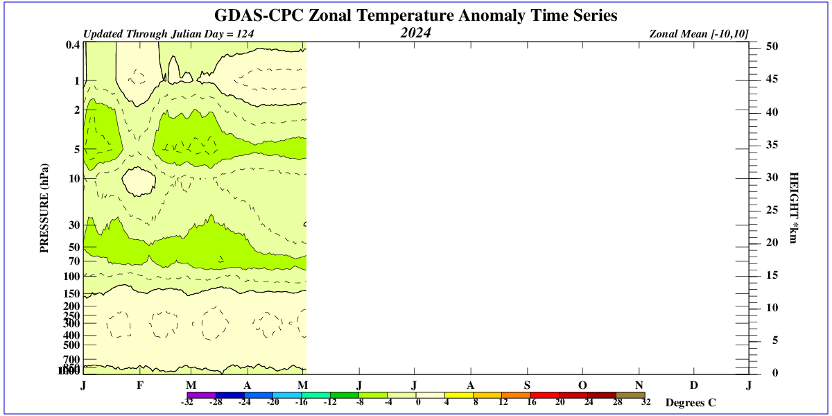
There’s a 3 year cycle embedded in the graph – anyone have an opinion on what would be causing that?