Kevin Kilty
Early last summer, during some internet search, Google’s AI Overview told me that Earth’s energy imbalance (EEI), that is the difference between incoming solar irradiance and outgoing solar plus long wave infrared, is 0.5 ± 0.47 W/m2. Like most facts that AI Overview offers, I gave it little attention at the time, but filed it away in my memory.
Later, I began to ponder the number. Several things occurred to me. First, the uncertainty seemed to me an attempt to avoid writing the value as 0.5 ± 0.5 and thus potentially including zero in whatever confidence interval was being expressed. After all, it is difficult to speak of the world starting to cook, when a confidence interval on the source of heat includes zero – i.e. no heat source at all. Second, the number is very small considering that at any given time in the temperate zones incoming solar irradiance might be over 1,100 W/m2 and is highly variable to boot. I wondered “How does one measure this imbalance number and how well can we characterize its uncertainty?” What I expected to learn was that EEI is a very small number when compared to the variability of climate, and that its magnitude is greatly uncertain.
It’s difficult to get AI Overview to repeat things at a later time, and there was no use searching for the original source of the 0.5 ± 0.47 W/m2 figure using it. I eventually located the origin of this value but learned that it referred not to the EEI per se. Rather, it was a measure of decade to decade change in EEI. Along the search, however, I found an array of EEI values at different places stated in different ways.[1] Estimates ranged from 0.47 W/m2 to 1.0 W/m2.
Some of this dispersion apparent in all these values can be explained as figures covering different time periods. For example, figures of 0.47 W/m2 and 0.76 W/m2 quoted by Von Stuckmann et al [2] are for the time periods 1971-2018 and 2010-2018 respectively. Nonetheless, this is a rather large dispersion of estimates for energy imbalance considering that one person described it as “ the most fundamental metric that the scientific community and public must be aware of as the measure of how well the world is doing in the task of bringing climate change under control…”
In addition, the values pertaining to uncertainty for this very important number are unclear. Are they one-standard deviation values, 95% confidence intervals, 90% values or something else? It turns out they are a mixture. Since a number of people argue that the EEI is increasing with time, are these mean values over some time period plus uncertainty that are detrended or are they instantaneous at some particular time? Many questions to answer.
Let’s see what we may learn in some selected literature research.
Energy accounting
Earth’s energy accounting is not terribly different from double-entry financial accounting. There is a revenue account (incoming solar irradiance) and the expenses of outgoing longwave and reflected solar irradiance. Meanwhile in our energy ledger we have an assets account where I would place any energy additions to doing useful things like warming the planet or greening it, but which alarmists would call the liabilities account, perhaps, and a Earth’s energy equity account.
However we might name these accounts, our double entry system must balance, and this should provide two independent ways of determining energy balance or lack thereof. In one way we look at the flows of energy crossing a boundary at satellite level. In the other method we look at all the places where energy appears to have accumulated. In principle the two ought to produce the same numbers to within the uncertainty of each.
Magnitude and Uncertainty
Since energy imbalance is one of many metrics being employed to argue for changes to livestyles, products, and the economy as a whole, it had better be proven to be a highly certain menace. At a minimum this means being accurately measured.
Uncertainty of a measurement is not merely a matter of the randomness of a process being measured or randomness in sampling of a population. It has to include all aspects of a measurement, from the inherent randomness of the process being measured, through uncertainties of instrument construction, calibration, drift, installation (think of the surface stations project here), algorithms, and data reduction. If a stationary process is sampled in a truly random fashion, then the dispersion of measurements might encompass all of the components of uncertainty.[3] Exceptions to this include systematic errors and bias. Errors and bias are a particular concern when specialized or unique instruments and platforms are involved, because this equipment, consisting maybe of only a few units, will not produce a statistical ensemble, and the biases are unlikely to be recognized in the measurement statistics alone.
In particular, Henrion and Fischoff found that measurements of physical constants tended to group near one another even when later, and better, measurements showed this grouping to be extremely unlikely.[4] They suggested this to be an artifact of the sociology of physical science. In one sense there was a conflict between a desire to produce the definitive work (small uncertainty) and the surety of being correct (larger confidence bounds) with the former winning out often. Another finding was that scientists did a poor job of evaluating bias and that supposedly independent research groups could be nudged toward a value found by the most influential group among them (Bandwagon effect). In climate science a similar nudge is produced by a desire to produce shocking results – an effect one might call this the “it’s worse than we thought” bandwagon.
Direct measurements of energy flow
A direct measurement of energy imbalance is available from satellite measurements. Nasa’s Clouds and the Earth’s Radiant Energy System experiment (Ceres) involved seven different radiometers flying on five different satellites beginning in 1997. These radiometers enabled direct measurement of incoming solar radiation, outgoing solar radiation, and outgoing LWIR. Two of these satellites had an end of operational life in 2023, but continued to operate afterward. Terra and Aqua are both now experiencing fuel and power limitations. A new addition to this experiment, Libera, is scheduled to fly early in 2028. This program has discovered some interesting things over the years.
In a September 2022 conference, Norman G. Loeb summarized the CERES mission, its findings, and some consequences of these findings.[5] According to this presentation, Earth’s energy imbalance has doubled from 0.5 ± 0.2 W/m2 during the first 10 years of this century to 1.0 ± 0.2 W/m2 recently. The increase is the result of a 0.9 ± 0.3 W/m2 increase absorbed solar radiation that is partially offset by a 0.4 ± 0.25 W/m2 increase in outgoing longwave radiation.
What do these uncertainty estimates mean and how credible are they? To answer the “what” part of this question, slide number 20 in the powerpoint is reproduced in Figure 1.

Figure 1. From Loeb, N. 2022 [5].
This shows a comparison of direct measures of in and out radiation against planetary heat uptake, which I will address next, but which amounts to an independent, indirect measure of radiance imbalance. The two measures trend closely together at 0.5 ± 0.47 W/m2 per decade. This slide reveals the source of AI Overview’s summary! The uncertainty is identified as a confidence interval (5%, 95%); so, ±0.47 translates to ±0.29 as a standard deviation. What looks good in this graph is the agreement in what we suppose to be two independent estimates of energy imbalance.
Further research shows this agreement to not be all it seems. Whatever coverage factor these ± figures refer to (𝞼, 2𝞼, 90% CI, 95% CI, etc), a number built from change in solar energy minus outgoing longwave would calculate to 0.5 ± 0.39 W/m2; this combined with 0.5 ± 0.2 W/m2 of a previous decade would equate to 1.0 ± 0.44 W/m2, not 1.0 ± 0.2 W/m2. Unless of course there is some negative correlation between and among them which is never explained. I have had real trouble making the figures I read consistent with one another. There’s more.
I began my research on uncertainty of the energy imbalance by referral back to a special volume of JGR from May 1986 dealing with the instrumentation for the predecessor of CERES which was the Earth Radiation Budget Experiment (ERBE).[6] There we find
“These instruments are designed to provide radiant flux and radiant exitance measurements to better than 1% measurement uncertainty over a 2-year orbital lifetime.”[7]
This source of uncertainty does not cover the total that is possible, but what is important is to compare this source of uncertainty with attempts to rectify CERES satellite estimates of EEI with ones based on heat uptake. In a paper the title of which explains a lot,”Toward Optimal Closure of the Earth’s Top-of-Atmosphere Radiation Budget,” we learn that calibrations of the instruments involved are accurate to 1-2%.[8] The underlying uncertainty of the instruments, themselves, doesn’t seem to have improved from ERBE to CERES.
There are two tables in this paper that are pertinent to our question of uncertainty. Table 1 from this paper shows the very large variations in imbalance of tens of W/m2 that are due to internal climate variability – variations which are far larger than credible EEI due to forcing. Table 2 from this paper shows a list of known and unknown biases. The known ones run the range from -2 to +7 W/m2, and that the EEI obtained from satellite measurements is too large by a factor of perhaps five to be credible.
While it seems that the intrinsic uncertainty of the instruments has not improved significantly from ERBE to CERES, there are improvements to the measurements of the energy budget that have come from correlations between CERES instruments, and other space platforms and ground truth. Irrespective of the cleverness of these schemes they bring with them uncertainties from other instruments, platforms and algorithms which should be propagated into results. I wished to see a full analysis of uncertainty somewhere, but I did not find one.
More concerning, though, is the discussion on algorithms to improve this circumstance for purposes of climate modeling by, in one case, making adjustments to LWIR radiance measurement and also different adjustments to SW radiance measurements in order to produce an EEI compatible with estimates of planetary heat uptake. The adjustments made at this time were not small but rather a factor of two larger than EEI itself.[9] In other words, estimates of heat uptake in the oceans and atmosphere have nudged the satellite measurements in a preferred direction. The two methods of estimating EEI are not independent of one another. We don’t really have a double entry accounting system.
Planetary Heat Uptake
Those places on Earth where excess energy might be retained are as follows: 1) Temperature change of atmosphere below tropopause, 2) Temperature change of oceans above 2000m depth, 3) Temperature of ground surface/subsurface and 4) Change to cryosphere temperature and phase change. A recent review of all this data and results can be found in von Schuckmann et al (2023).[2] Some estimates are truly remarkable with a claimed relative uncertainty below 10% (uncertainty divided by expected value) considering that 2) through 4) are places hidden from direct measurement.
However, the authors appear to recognize their uncertainty estimates are not so rosy. They say
“The ensemble spread gives an indication of the agreement among products and can be used as a proxy for uncertainty. The basic assumption for the error distribution is Gaussian with a mean of zero, which can be approximated by an ensemble of various products. However, it does not account for systematic errors that may result in biases across the ensemble and does not represent the full uncertainty.”
Nonetheless, we are told in perhaps the most optimistic case that the present rate of heat uptake is 0.76 ± 0.1 W/m2 [2] or perhaps as good as 0.77 ± 0.06 W/m2[10]. These figures come from adding up the totality of contributions 1) through 4) in our list; though 89% is from the ocean alone. The indicated uncertainty should come at least from adding the respective uncertainties of the contributors in quadrature, just as though these data are uncorrelated, independent and unbiased estimates of the same thing.

Figure 2. Storage of energy imbalance in the ocean. From K. von Schuckmann et al. (2023) Heat stored in the Earth system 1960–2020, © Author(s) 2023. This work is distributed under the Creative Commons Attribution 4.0 License.
The gigantic effort of accounting for where all the energy imbalance goes done by von Struckmann et al [2] which involves 68 co-authors at 61 institutions is an avalanche of data stated in various units, over different time periods, and coming from numerous sources and subsets of sources. It is extremely difficult to sort out. Figure 2 shows just one example of what I see as discrepancies in the compilation. Compare, for instance, heat stored in the ocean from 1960 to 2020 to heat stored from 1993 to 2020. The depth range 0-2000m surely is made from the sum of 0-700m and 700-2000m as the sums in each case clearly show. Yet the uncertainty figures are impossible to reconcile. In one case uncertainties of 0.1 and 0.04 combine to 0.1 and in the other case the same combine to 0.2. Maybe there is covariance between the two depth ranges; though Figure 2 in Von Schuckmann et al [2] shows obvious positive correlation in all depth ranges – something that should amplify uncertainty not reduce it.
Acceleration of EEI
One prominent theme of all this work on energy imbalance is that the heat uptake is accelerating. Loeb et al [10] suggest that satellite observations show energy imbalance has doubled from 0.5±0.2 W/m2 during the 2000 to 2010 time period to 1.0±0.2 W/m2 during the 2010 to 2020 period – what I’d call decadal estimates. The increase is the result of a 0.9±0.3 W/m2 more absorbed solar radiation, partially offset by 0.4±0.25 W/m2 increase in outgoing longwave radiation.
Once again I face some troubles making all of this consistent. One would infer the result of increasing solar radiation and also increasing outgoing LWIR, here, by the rules of adding uncorrelated estimates, to be 0.5±0.4 W/m2, but which Loeb [5] characterizes as 0.5±0.47 W/m2, with a (5% – 95%) confidence interval. It’s puzzling.
Von Struckmann et al [2] suggest the equivalent decadal numbers to be 0.48±0.1 W/m2 and 0.76±0.2 W/m2 (which uncertainties they call a 90% confidence interval, 5%-95%), which are, if the stated uncertainties are to be believed, far smaller than what Loeb et al [10] calculates.
Neglecting all the differences, however, it is apparent all groups are presenting evidence of accelerated imbalance. Is this well established, though?
I decided to perform a little experiment with the uahncdn_lt_6.0 dataset (University of Alabama, Huntsville). I used an ordinary least squares linear regression. The month to month linear coefficient of increase is 0.0013C, and the 95% confidence interval runs (0.0012 to 0.0014 C/month). Figure 4 shows this. As Dr. Spencer has written on his blog, this 0.02C change per year is what results from increased CO2 forcing and anything departing from it is some influence of climate variability.
A close inspection of Figure 3 indicates the data are not randomly scattered about the best fit line. Their trend looks rather flat near the origin and at several places there is a bit more data below the line than above. Some extreme values occur at the end of the time series. This shape suggests some curvature like a squared term.

Figure 3.
So, I fit a quadratic function only to the data (small diagram in the upper left of Figure 3), and got what seems to be a remarkably good fitting curve that has zero slope at the origin and rises monotonically to the end. Ah! Evidence of an accelerating trend?
Not quite.
The fraction of variation explained by a line is 51% and by a quadratic is 53% – an insignificant difference. The standard error of residuals is no different (0.198 versus 0.195), and one suspects that the data don’t quite meet the requirement of being independent and identically distributed across its domain. In fact, it is simple to show there is correlation in this data across multiple time scales, and the correlation alone might fool a person into seeing a trend not there. This tendency toward a flattening followed by a brief but sharp rise appears in other data covering the entire past century as well, say 1920-1945. These temperature data are much too variable to establish a preference for the quadratic trend over the linear one.
Conclusions
When I began this effort I expected to discover that my search for energy imbalance would find a very small number with a very large uncertainty. This is exactly what I found. In addition, I was surprised to see that estimates of heat uptake provided a large nudge to satellite data, which leaves the estimates not independent. I also should have figured that whatever value of EEI that resulted would serve some purpose in promoting worry over climate change.
Something that all investigators in this EEI community do is tie energy imbalance to a litany of problems in the present world. To them a warming planet is nothing but trouble; there seems no upside at all. Von Schuckmann et al [2] even go so far as to calculate, from their estimates of imbalance, and even considering the acknowledged unknown uncertainties and assumptions involved, how much CO2 would have to be removed from the atmosphere to bring us back to year 1988, or to keep the Earth below 2C temperature change from the late 1800s. Why these two goals are important isn’t clear but we are told that they somehow will prevent climate problems.
But issues that cause panic are not related to puny temperature change. Heat waves do not arise from a 1C or even 1.5C background temperature rise. They arise from UHI approaching 10C and resulting from the way we have constructed our mega-cities, which are full of energy dissipating equipment and cut off from countryside breezes. Sea level rise, being puny, does not cause flooding – failures of civil engineering and people building in places they shouldn’t are what cause flooding. Knowing the EEI, which might be interesting in its own right, will aid in preventing none of this.
References:
1- See for example: Trenberth, et al, Earth’s Energy Imbalance, Journal of Climate, 27, 9, p.3129-3144, 2014 DOI: https://doi.org/10.1175/JCLI-D-13-00294.1; V. Schuckmann, et al, Heat stored in the Earth system: where does the energy go?, Earth Syst. Sci. Data, 12, 2013–2041, https://doi.org/10.5194/essd-12-2013-2020, 2020; Loeb, N.G., et al. Observational Assessment of Changes in Earth’s Energy Imbalance Since 2000. Surv Geophys (2024). https://doi.org/10.1007/s10712-024-09838-8;
2-v Schuckmann, et al, 2023, Heat stored in the Earth system 1960–2020: where does the energy go? System Science Data, 15(4), 1675-1709. https://doi.org/10.5194/essd-15-1675-2023
3 -Guide to Uncertainty in Measurement. Available online at https://www.bipm.org/documents/20126/2071204/JCGM_100_2008_E.pdf
4-Max Henrion and Baruch Fischoff, Am J. Physics. 54,791, 1989. See also Science. 289, 2260-2262, 29 September 2000.
5-Loeb, Norman, Trends in Earth’s Energy Imbalance, ISSI GEWEX Workshop, September 26-30, 2022, Bern, Switzerland. Powerpoint online at: https://ntrs.nasa.gov/api/citations/20220010511/downloads/Loeb_2022_compressed.pptx.pdf
6-B. Barkstrom, and G. Smith, The Earth Radiation Budget Experiment’ Science and Implementation, Reviews of Geophysics, v. 24, n 2, p. 379-390, May 1986
7-Kopia, L. Earth Radiation Budget Experiment Scanner Instrument, Reviews of Geophysics, v. 24, n 2, p. 400-406, May 1986
8-Loeb et al, 2018, Clouds and the Earth’s Radiant Energy System (CERES) Energy Balanced and Filled (EBAF) Top-of-Atmosphere (TOA) Edition-4.0 Data Product, Journal of Climate, DOI: 10.1175/JCLI-D-17-0208.1 “With the most recent CERES edition-4 instrument calibration improvements, the net imbalance from the standard CERES data products is approximately 4.3 , much larger than the expected EEI.“
9-Loeb, et al, 2009, Toward Optimal Closure of the Earth’s Top-of-Atmosphere Radiation Budget. J. Climate, 22, 748–766, https://doi.org/10.1175/2008JCLI2637.1.
10-Loeb, et al, 2024, Observational Assessment of Changes in Earth’s Energy Imbalance Since 2000. Surveys in Geophysics; https://doi.org/10.1007/s10712-024-09838-8
So I need some clarification. My understanding is that measurements such as CERES do not adequately capture the far infrared outgoing radiation. This was the whole point of the RAVAN satellite project which seems to never really have been implemented. Far infrared us estimated to be half of outgoing energy? But who knows until we measure it. So if we can’t know for sure we are measuring all the outgoing energy, we can’t know the budget/imbalance.
You sent me off to research RAVAN. It appears to have been a demonstration project and these often have trouble going further because of a lack of advocacy. What is the wavenumber range of Far IR that you are speaking of?
Even if we knew the exact budget/imbalance it would still be a problem relating that imbalance to a temperature difference. If the IR radiation is related in any way to Planck and/or S-B then it has at least a polynomial relationship to temperature. Without knowing all the factors of that polynomial any tie-in to temperature will be a guess at best. Guesses have an in-built uncertainty that must be accounted for – except in climate science.
The more important questions-
Where is the imbalance and why.
The first is to distinguish between heat “uptake” and heat “retention”. Oceans are retaining heat. They are not cooling as fast. The greatest heat retention is in oceans at 45S:
 ?ssl=1
Note that the majority of the retained heat is in the region of the Ferrel Cells. These are radiation net heat loss zoners. So the ocean heat is being retaining through increased net precipitation in the region of the Ferrel Cells. Nothing to do with CO2.
As the peak sunlight moves northward, the land and oceans in the northern hemisphere warm up causing more atmospheric moisture. That is increasing heat advection from the tropics to the poles in both hemisphere. But Southern Hemisphere is getting less sunlight so the increased heat advection is not increasing the temperature like the NH that is getting more sunlight.
Averaging over the entire globe washes away pesky variations.
Their measuring methods, cloud cover, satellite footprint, surface temp variation,weatherchanges during orbital time, atmospheric water vapor, and the list goes on…..simply don’t allow them to say they have anything like 1/2 watt accuracy, 10 watts more likely…Sure their individual instruments might be calibrated to some standard repeatable to maybe .1 watts
Think of having a tape measure a hundred meters long accurate to 1 mm….that you are using to measure the distance between wave crests on a pond on a stormy day from a moving boat. The result of your readings are just never going to be accurate to 1 mm.
So what the climate guys do is start with a degree rise in one century of weather records and fudge the depth of ocean warming to confirm the temperature rise they assumed to start with. Confirmation bias and circular logic all rolled into one.
Something that all investigators in this EEI community do is tie energy imbalance to a litany of problems in the present world. To them a warming planet is nothing but trouble; there seems no upside at all.
Tell me something I don’t know-
Adelaide records coldest minimum temperature in 100 years (msn.com)
I’ll bail up the next aboriginal elder I see and compare notes but thank God for Nikola Tesla and Mitsubishi Heavy Industries and all is forgiven for bombing Darwin and Broome in my folks’ time.
Kevin,

Many thanks for drawing attention to this serious and fundamental set of problems.
The views of people are coloured by their experiences, of course. Those of us who were exposed to the analytical chemistry lab will find your article familiar, while those with arts/history type degrees will likely have a blank stare. Here is my lab in 1969 when professional gentlemen wore ties. Pat Frank understands this material from his lab days.
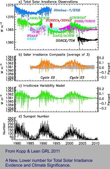
I first started ranting about the energy imbalance problem with the following image soon after publication of papers by Kopp 2011 and Butler 2008. Laboratory training or not, any analytical scientist has to know about the uncertainty of a tiny number derived from subtractions of two large ones. Also, knowledge is required of “adjustments” when overlapping time series data do not match. Here is a classic, important case that is part of this WUWT article.
Many papers have been written about how to synchronise these various satellite platform tracks and their adjustment. Kevin lists some of the more important papers. Many of them deal with the old-fashioned term “precision” Some, the important ones, address “accuracy”. Here, there is a barrier. Nobody knows the definitive, best accurate answer for the difference in energy in and out, so all past adjustments are subjective. There is likely to be a new ball game when the next, improved satellite starts transmitting – as has happened before, Kevin’s reference 8.
Suggestions? Read. Learn and digest what Kevin noted, particularly his reference 3 for uncertainty.
Do not trust adjusted data too much. Problems similar to this one are to be found in other parts of climate research, such as satellite ocean levels, calculation of “anomaly” temperatures and more.
Geoff S
I never worked with any equipment that looked like yours, Geoff! 🙂
I’ve always understood the surface warming phenomenon to be explained, as that the greater heat energy in the atmosphere increases the height at which the tropospheric LWIR radiates off into space.
A constant lapse rate means the higher radiant altitude requires the surface to warm. A 0.6 C increase in sensible heat at the surface translates into a 0.1 km increase in radiant altitude.
Higher altitude of radiation loss, at constant energy flux, means the radiant surface area must increase. Increased radiant surface means the intensity of the LWIR decreases, but the total energy radiated into space stays constant.
So, the question is, is the lower intensity of LWIR (constant total energy flux) being interpreted as lower emitted energy? Is the EEI really just an unaccounted artifact of a larger radiating surface area?
That is a common explanation that is correct in a sense and maybe useful, but is also misleading in another sense, I think. I can even come up with a model that says the ground surface is both in the inbound and outbound boundary of the problem.
The surface, water or solid, is condensed matter and radiation leaves it in a thermal spectrum, or darned close to one (e=0.97). Some of this thermal spectrum is in clear windows and transported out, ballistically, to space. So, the surface itself is part of that “layer” transporting heat energy to space. In the 15um CO2 band radiation goes just about no place before CO2 gets hold of it — pretty much absorbed in 100m of air. It is released from CO2 in a number of ways. Some energy rises in the atmosphere and engages in other interactions. Some manages to reach the ground surface again– it’s the greenhouse effect.
Once it’s absorbed again on the surface it loses its identity and becomes a part of the thermal spectrum once more, a portion of which is in the clear and transported to space. The lower boundary of the outbound LWIR is the surface, but this “upper boundary” is the entire atmosphere. Yes, an enhanced green house effect raises the average height of the outbound radiation, but you can see that the idea of a layer at height which will rise with increasing CO2 is a stretch as far as an explanation goes. It’s more complicated.
Up where I live at 2300 meters the air above is 25-30% transparent, so a person could say, as an explanation, that 3-4 bounces of radiation to the surface and back up again and it leaves the planet; it’s an expected value, but the situation is still more complex. The interaction of radiation with matter is simply complex and any simple model gets a little bit right and a lot wrong.
That is JCGM 100:2008.
I’ll repeat my questions to you for the 3rd time [1][2]…
Do you accept that the NIST uncertainty machine, which uses the technique specified in the GUM document (JCGM 100:2008) produces the correct result when given the measurement model y = f(x1, x2, …, xn) = Σ[xi, 1, n] / n or in the R syntax required by the site (x1 + x2 + … + xn) / n?
Do you accept that the uncertainty evaluation techniques 1) GUM linear approximation described in JCGM 100:2008 and 2) GUM monte carlo described in JCGM 101:2008 and JCGM 102:2011 produce correct results [JCGM]?
It’s been pointed out to you multiple times that GIGO with the NIST machine.
Put in a mult-modal distribution with different standard deviations for each mode. The NIST machine will give you an average and a standard deviation around that average.
What do you think that is actually telling you?
It’s what the NIST machine will tell you when you combine southern hemisphere temps with northern hemisphere temps – which are multi-modal since one hemisphere will be in winter when the other is in summer.
Again, what do you think the NIST machine is actually telling you in such a case?
Still cherry-picking the uncertainty literature to “prove” that averaging air temperatures makes measurement uncertainty go away, and increases the resolution of 1°F measurements.
They don’t.
The formula for averaging a series of values is NOT a measurement model.
This is your invention.
I don’t think he is *EVER* going to understand that! The average of a series of values is a statistical DESCRIPTOR. It is not itself a measurement. It’s only purpose is to allow better understanding of the distribution. It *must* have all the other applicable statistical descriptors given as well in order to understand the distribution, e.g. variance, skewness, and kurtosis. The average by itself is truly meaningless since it doesn’t fully describe the distribution.
But somehow climate science never really bothers even with the variance.
He refuses to even consider that he might be wrong—doing so would jeopardize all the GAT numbers published in the climate journals that he holds sacrosanct.
The GAT is a joke. He forgets that when you subtract random variables (monthly average – baseline average), the standard deviations add. Note, not one resource I could find anywhere said the SEM’s add, only the SD’s.
He doesn’t forget—after having been told this over and over; it is entirely intentional.
You got that correct. He hasn’t shown how he can get 30 “inputs” for a monthly average into the UM that limits you to x0 – x14. You either use GUM Eq 3 and 4 ahead of time, or input sample values. I’ll guarantee that that 30 daily temperatures won’t have its standard deviations divided by 30 a second time.
It is Equation 3 in the GUM.
bdgwx has ignored the fact that a group of measurements of the same or similar things is a random variable that has a mean and standard deviation.
He has never learned that f(X1, …, Xn) depicts random variables of different measurements that combine in a measurement model. IOW, X1 = length and X2 = width and X3 = height.
When your measurand is AVERAGE monthly temperature, that is ONE random variable with ≈ 30 entries that has a mean μ and an SD σ. The SD is the uncertainty of the average.
The SD that climate science routinely ignores and tosses in the recycle bin.
The Uncertainty Machine requires a distribution and standard deviation or a sample of measurement data from which it calculated the necessary distribution data.
For each of the inputs to the UM, there is a μ (mean) that has already been divided by “n”. The deviation has already been divided by “n-1” during each input distribution calculation.
Your measurement model is incorrect from the standpoint that dividing by “n” is already implicit in the values of the inputs.
You are cherry picking equations to get the answer you want. Typical of climate science.
Equations 3, 4, 5 in the GUM specify how to calculate the mean and standard deviations appropriate for Gaussian distributions of random variables that are input to the UM for each unique measurement used to calculate the measurand. Other sections discuss other distributions.
As a learning experience, read through all the examples shown and tell us how many of the measurement models use the division by the number of data points in each measurement for each input.
As a check, take the temperature measurements of TN 1900, add eight or nine to the group in the middle to end up with 30 data points. Use the sample choice of the UM to see what you get.
I’m not entirely sure what you are saying, but you say “measurement model” and then use this example
y = f(x1, x2, …, xn) = Σ[xi, 1, n] / n or in the R syntax required by the site (x1 + x2 + … + xn) / n
But what this implies is just the calculation of an arithmetic mean of (n) measurements. The form of f() is very important. It’s what we call the “measurement equation” and it plays a central role in the propagation of uncertainty. In the specific case of planetary heat uptake the measurement equation is PHU = X1+X2+X3+X4; its the sum of four contributors, not a mean value. Thus, in the simplest possible case, assuming independence of the four contributors, we obtain the over all uncertainty by summing variances (uncertainties squared) and then taking a square root to get the resulting one-sigma standard uncertainty of PHU — it obviously must be larger than the sum of the four standard uncertainties.
Tell me what you interpret this to be in a more complicated example.
Great post Kevin.
A number of us have tried to get this across to bdgwx, bellman, and others. Section 4 in the GUM details how a measurand is developed. Specifically,
In essence, a measurand of monthly_average has a measurement model of f(X₁,ₖ). X₁,ₖ is a random variable made up of ≈ 30 data points. That is, {X(₁,₁), …, X(₁,₃₀)}. The mean is determined by Equation 3 and the the standard deviation by Equation 4.
Good luck in convincing them.
The NIST UM also uses the distinct definition of “input quantity”.
I doubt you will ever get an answer.
A statistical mean is a *statistical* descriptor. It is not a functional relationship. A functional relationship uses physical properties to calculate a physical property, e.g. the radius and height of a barrel to calculate its volume, using the charge enclosed by a surface to calculate the electric flus through the surface, using the volume and mass of an object to determine its density, …..
An average is *not* a measurement equation unless you are a statistician or climate scientist. An average is the central tendency of a probability distribution, it is not a measurement. Statistics calls the average an “expected value”. It’s like saying the expected value of the volume of an isolated barrel is 50 gallons because that’s the most common size barrel. That is *not* a measurement of that barrel. That isolated barrel may be a 5 gallon, 10 gallon, 25 gallon barrel or many other values. But you don’t *know* what it is unless you measure it and use a functional relationship to find the volume.
That’s the big problem with the “global average temperature”. It’s *not* a measurement even though climate science treats it as such. It’s an average of averages derived from other averages. It’s an “expected” value determined from “expected” values that are derived from other “expected” values. “Expected” values are nothing more than phantom swirls in a cloudy crystal ball. They are *not* measurements.
As the GUM says:
“uncertainty (of measurement)
parameter, associated with the result of a measurement, that characterizes the dispersion of the values that could reasonably be attributed to the measurand”
An average does *NOT* characterize the dispersion of values that could reasonably be attributed to the measurand. How many digits you use in calculating the average does not characterize the dispersion of values that could reasonably be attributed to the measurand. The sampling error (i.e. the SEM) does not characterize the dispersion of values that could be attributed to the measurand, it only tells you how precisely you have located the mean.
Sorry for the diatribe. I just get irritated at the pushing of the misconception that an average is a functional relationship.
JCGM calls it the “measurement model”. [JCGM 200:2012, 2.48, pg. 32]. They even have a whole document dedicated to explaining and providing examples of measurement models and how to deal with them. [JCGM GUM-6:2020]. They can be arbitrarily complex with models stacking on top of other models which themselves can include more than just a trivial equation which may include complex heuristics, statistics, algorithms, etc.
Sure, that’s one measurement model for assessing PHU. Others exist as well. And although interesting in its own right note that the measurement model you provide here has a different form than the one I asked Geoff about so it isn’t really relevant to the question I posed for Geoff.
Correct. And if they aren’t independent, but have positive correction r(Xi, Xj) > 0 then the uncertainty will be even larger. Again, note the example you provided is not of the same form as the one I used in my question for Geoff so it isn’t particularly relevant.
In regards to my question posed to Geoff…
Consider a set of N different equally sized solar panels deployed in a similar manner. You want to know the average efficiency fraction for the set in your possession so that you can quickly assess the total power output from that set given a specific solar irradiance.
(1) Given the individual efficiency fractions Xi for each panel and their uncertainty u(Xi) what is the formula for the uncertainty u(y) where y = f(x1, x2, …, xn) = Σ[xi, 1, n] / n is the average efficiency fraction of the set?
(2) Using the formula from (1) what is the uncertainty u(y) given the concrete example where x1 = 0.3 ± 0.04, x2 = 0.3 ± 0.04, and x3 = 0.2 ± 0.04 where the value after ± is the standard uncertainty u(xi)?
(3) Going further…given the total area of the 3 panels in (2) of 3 m^2 ± 0.1 and solar irradiance of 500 W.m-2 ± 10 W.m-2 where the values after ± are the standard uncertainty u what is the total power delivered by the system using the average efficiency calculated in (2)?
The uncertainty of the average efficiency of those panels is the dispersion of values that could be assigned to the average efficiency at any moment in time.
That is *NOT* the average efficiency.
The measurement uncertainties of the panels will ADD, perhaps in quadrature. They will not “average*.
The total power delivered at any point in time will be the sum of the estimated power output of the four panels at that point in time. The uncertainty of the power delivered will be the sum of the measurement uncertainties associated with those estimates of power output.
If an one point in time:
Panel 1 output: 25 +/- 5
Panel 2 output: 23 +/- 4
Panel 3 output: 26 +/- 6
Panel 4 output: 22 +/- 2
The total estimated power output would be 96.
20 + 19 + 20 + 20 = 79 on the low side
to 30 + 27 + 32 + 24 = 113 on the high side
So you would expect to get 96 +/- 17
(you can add the uncertainties in quadrature if you like but with only four components just how much cancellation would you expect?)
If you want to know what to expect during the entire daylight hours then calculate what the estimated outputs would be along with the associated measurement uncertainties over the daytime profile (e.g. sun angle, etc).
That will create a distribution of values from which you can calculate an average value plus a dispersion of values around that average that could be reasonably assigned to that average value. It will *NOT* be the average measurement uncertainty nor will it be the SEM.
If nothing else, calculate the average output power and then look in the distribution elements for the nearest value to that average and use the measurement uncertainty for that value in the distribution!
If the point in time calculated above turns out to be the nearest to the average output then your average power output would estimated at 96 +/- 17. It would *NOT* be 96 +/- 4 where 4 is the average measurement uncertainty at that point in time.
He won’t understand, because it would require jettisoning his preconceived notions.
Liar, it does no such thing; this is your invention to prop up your bullshit claims of tiny milli-Kelvin air temperature “uncertainties”.
Rest of insane rant skipped.
complicated
Yes. Let’s make it more complicated. Here is a bonus challenge.
(4) Similar to question (3) above except here show how the total power delivered is calculated (and specifically the uncertainty of it) by using the individual efficiency fractions specified for each panel from question (2) as opposed to the average efficiency fraction of the set.
Fair warning…this is more complicated than it may initially seem because of the information provided. But it is possible.
I have crafted this example and questions 1-4 to demonstrate multiple salient points that are misunderstood by some authors and participants of WUWT
I told you how to do this already. Did you not bother to read my reply?
The solar radiance is a continual function whose factors include the path of the sun (sin(x)) and the transiting media. The conversion efficiency will *NOT* be single value, it will change over time as the angle of incidence changes and the weather (i.e. clouds) changes. The conversion efficiency will even change with the amount of dust, snow, or ice that is on the surface of each panel.
This all contributes to the uncertainty associated with the power delivered at any point in time.
This is a perfect example of why degree-day values are a far better metric for measuring climate than is temperature.
In this case you would be far better off actually measuring the output curve over an extended period. If I were engineering this project I would go out looking for data that has already been collected for a similar location and similar equipment. There are far too many factors with uncertainty to allow theoretical calculations without also having a wide uncertainty interval in the final answer. It’s one reason why the supposed power delivery of solar and wind installation *NEVER* live up to expectations.
Which is exactly how is it done, measuring the power output as a time-series and integrating it to get energy.
You know if the two Gormans, Karlomonte, Pat Frank, and Geoff can’t convince you of anything I am not sure my effort will do anything more. And answering this is a lot of trouble. So, until Part II, if I ever get to it, this is my last comment on Part I.
First, from your explanation you are asking for the mean efficiency of some small batch of panels. The problem, from the standpoint of uncertainty, is not fully specified. Are we 1) actually measuring each panel as would be done in an industrial QA/QC sort of “experiment”, or are we 2) estimating the measured efficiency of a panel, not yet constructed, but having particular design characteristics, manufactured according to the capability of our process when it is in control? In either case there is the additional uncertainty introduced as tested by a technician with a single recently calibrated instrument who might not connect each panel to the apparatus with repeatability. This is the issue in mass manufacturing. Look up statistical process control (SPC), Gage R&R, and process capability to get an idea of what we are speaking of.
For sake of simplicity, assume option 1). There is no uncertainty before we have measured each element of the batch except for the distribution attached to our process capability. When we are done we calculate average efficiency according to your formula. For a calculation of expected uncertainty we would simply use the formula for variance of the measurements.
where gamma is the covariance within the sample. This covariance exists because there is correlation from one panel to another in our manufacturing process because as long as it stays within the SPC limits we don’t adjust to target, and because the QA/QC test person has some procedure for organizing the test that will add some error and correlate results from one item to another. If there is no correlation present then this reduces to the result so often used inappropriately that
Now off to the second challenge. What is the expected power output of the array of cells? The power output is now not an average, but rather a summation of n cells connect in the field. We have a pretty good idea of how to characterize each cell because of the previous result. Our measurement equation is now Power=X1+X2+X3+…-Loss. The loss term comes from the capability of the field engineers/contractors to put the array together correctly, orient it correctly, etc. Previous experience would have given us an expected value for Loss and its uncertainty. To calculate the uncertainty of the as constructed field array we’d add the variances of each term including Loss (these variances may contain covariances that are not zero), and then take a square root to get a standard error. However, the field installation may involve a further “acceptance” test, and this would bring further uncertainty with it because of skill of the QA/QC people and their instrumentation.
It is easy enough to foul-up the acceptance test as the original troubles with Hubble Space Telescope demonstrate.
I have not put any numbers to this because a huge amount of the calculation involves experience (Loss, capability, etc) which is unspecified at present.
Oh…so you support them? That is a twist I didn’t see coming.
I’m curious how far your support goes with the Gormans…
Do you also agree that d(x/n)/dx = 1?
Do you also agree that Σx/n = Σx?
Do you also agree that PEMDAS rules can be ignored?
Do you also agree that a/b = b?
Do you also agree that Σ(a^2) = (Σa)^2?
Do you also agree that sqrt[xy^2] = xy?
I’m curious how far your support goes with Pat Frank.
Do you also agree that Bevington equation 4.22 and not 4.23 is the formula for the uncertainty of the average?
But yeah, if your support goes this deep then you are going to have a very hard time convincing me.
Everything is specified. They are not trick questions. In fact, it is an example that is meant to be brutally trivial and simple.
Agreed. But that’s not what the two Gormans, Karlomonte, and Pat Frank say it is. I don’t know about Geoff yet. He seems to want to remain non-committal.
Agreed. But again, that’s not what the Gormans and Pat Frank say it is. I don’t know about Geoff. And I think karlomonte mostly just repeats what they say just with clever ad-hominems to spice things up.
The Gormans want me to think it is u(x) = sqrt[ u(x1)^2 + … + u(xn)^2 ].
Pat Frank wants me to think it is u(x) = σ_x or in [Frank 2010] u(x) = sqrt[ n*σ^2 / (n-1) ]. Note that lim[ sqrt[ n*σ^2 / (n-1) ], n to ∞] = σ. BTW…this isn’t strictly wrong, but you have to assume that r(xi, xj) = 1 which would only be true if each xi had the exact same error. Pat later told me he used Bevington equation 4.22 which is the problem. Bevington clearly articulates that the uncertainty of the mean should be calculated via 4.23. 4.22 is only an intermediate step. Nevermind that 4.22 and 4.23 are part of the procedure when dealing with relative uncertainties as Bevington starts discussing on pg. 57 which isn’t relevant when dealing with absolute uncertainties which is how most uncertainties are specified and propagated.
That’s the question. Given x1 = 0.3 ± 0.04, x2 = 0.3 ± 0.04, and x3 = 0.2 ± 0.04 where xi is the efficiency fraction for each panel, the total area of the 3 panels is 3 ± 0.1 m^2, solar irradiance is 500 ± 10 W.m-2, and the values after ± are standard uncertainty u what is the expected power out of the array? Assume r(xi, xj) = 0 for each combination of panels (it’s a trivial example). You have anything you need to answer the question.
Sure. That’s a perfectly fine measurement model. But, given the information provided that’s going to be harder to calculate. See the bonus challenge (4) above. I think once you go through the motions you’ll see why its hard and why doing as specified in question (2) is easier at least in this particular case. Both measurement models yield the exact same result.
You have everything you need to answer the questions. I answered both questions 3 and 4 using both the NIST uncertainty machine and hand calculation using JCGM 100:2008 equation 10. Give it a shot. I suspect you’ll get the same answer I did based on some of your comments so far. I have some concerns that if you truly agree with the Gormans you could commit trivial algebra mistakes, but I think that is unlikely and sense that your statement of support of them is probably more of a blind off-the-cuff knee-jerk remark that has significant and materially impacting limits.
The uncertainty of (x/n) is the uncertainty in “x” plus the uncertainty in “n”.
Consequently, (d/dx)x =1 and (d/dx)1/2 = 0.
As Dr. Taylor points out, the uncertainty in division is the uncertainty of each component added together.
Fundamentally if you have “a/b”, the uncertainty is δa + δb. u(a) = δa and if b= 1/2 then u(b) = δ(1/2) = 0. So you get δa + 0 = δa
There is no reason to deal with any of your other mathterbation if you can’t get understand the basics of measurement uncertainty.
stop your cherry picking for things you don’t understand.
Take Bevington 4.21, 4.22, and 4.23. They are being used to find u”.
Guess what u” is? It’s an estimate of the MEAN. From the text right before 4.22 – “To find the error in the estimate u’ of the mean we must calculate a weighted average variance of the data:”
Exactly what do you think the “error in the estimate of u’ of the mean” IS?
It is *NOT* the measurement uncertainty of the mean. It is the STANDARD ERROR OF THE MEAN!
In fact, if you go back to the beginning of the section titled “Estimated Error in the Mean” Bevington states:
“What uncertainty σ is associated with our determination of the mean u’ in Equation (4.9)? We have assumed that all data points x_i were drawn from the same parent distribution and were thus obtained with an uncertainty characterized by the same standard deviation σ. Each of these data points contributes to the determination of the mean u’ and therefore each data point contributes some uncertainty to the determination of the final results. A histogram of our data points would follow the Gaussian shape, peaking at the value u’ and exhibiting a width corresponding to the standard deviation σ. Clearly we are able to determine the mean to much better than +/- σ, and our determination will improve as we increase the number of measured points N and are thus able to improve the agreement between our experimental histogram and the smooth Gaussian curve.” (bolding mine, tpg)
Bevington is talking about more precisely locating the mean and *NOT* the measurement uncertainty of the mean.
Remember, this entire portion of Bevington’s book is addressing PURE RANDOM ERROR – no consideration of systematic bias in measurement instrumentation or measurement procedure. Thus this all only applies to situations where you have perfectly repeatable measurements, i.e. multiple measurements of the same thing under the exact same environment using the exact same instrument.
Therefore this simply does not apply to temperature measurements from multiple different instruments making single measurements of different things – i.e. the GAT or any of the data sets used to find the GAT. How precisely you can locate the average is simply not a valid determination of the measurement uncertainty.
I’m not even going to address the other points. You can’t even state what you’ve been told over and over on how to do metrology in an accurate manner. Your understanding of measurement procedures and the uncertainty propagation associated with them is totally lacking, all you know is Stat 101 where there is *NO* consideration given to the data sets being analyzed having elements with uncertainty. So all you fall back on is the meme that all measurement uncertainty is random, Gaussian, and that it all cancels. Therefore the sampling error becomes the uncertainty of the average.
Your long list of “Do you also” questions look like the answer is “no”. Perhaps a trick question. I don’t know the history of controversy here. Maybe they are one-time errors. I have made plenty of errors in my life. I have seen plenty of algebraic errors in my time — I’ve had over 5,000 engineering students after all.
What I am refering to is this. They are trying to get you to see that uncertainty (propagation of error as it was once known) is not the same as standard error of the mean except in rather special circumstances.
To your specific challenge, I did not use the so called NIST “machine” but rather used only eq. 10…I end up with 400 ± 42.4… Bigger than a bread box, smaller than Texas.
100%
Btw, 400 +/- 42 is about a 10% measurement uncertainty. That’s not very good for trying to pin down differences in the units digit or in a decimal place.
I make more than my fair share mistakes. I can guarantee I make more than you do. I’m often sloppy with arithmetic and algebraic operations so I frequently use a computer algebra system to verify my work because I’m so prone to mistakes. And I almost always verify uncertainty calculation results with the NIST uncertainty machine. It is especially helpful when non-zero correlations are involved.
Unfortunately no. The algebra mistakes are frequent and repeated. Some of the math is non-trivial like the partial derivatives in JCGM 100:2008 equation 10. After showing how to algebraically evaluate the partial derivative of a function and even showing CAS solutions(see here and here) they still think ∂f/∂xi = 1 when f(x1, …, xn) = Σ[xi, 1 to n] / n. And then in defense of their mistakes in the harder realm they start making trivial mistakes like sqrt[xy^2] = xy. This goes on ad-infinitum. I (and others) occasionally engage in hopes that we can convince them of the correct math, but so far out attempts have been futile. I present to you this exhibit and all the absurdity it entails in this very blog post as example. Maybe you’d have better luck in explaining this stuff to them?
It’s actually the opposite. I (and others) have been trying to get them to understand propagation of uncertainty using JCGM 100:2008, NIST TN 1297, UKAS M3003, etc. for years. Bellman, another frequent poster, has been at it longer than I have.
Yep. Close enough. I got 400 ± 38 W.m-2 using both the measurement model in question (2) and the measurement model in question (4). I also verified this result with the NIST uncertainty machine again using both measurement models. The difference between our results may be due to rounding errors.
BTW…for the lurkers…the reason why challenge (4) above is deceptively complicated is because it requires the uncertainty of the area of the panels individually, but I only provided the uncertainty of the total area so you have to use JCGM 100:2008 equation 10 in reverse as an intermediate step. There are, of course, other ways to do it, but I’m trying to stick the method of propagation of uncertainty defined in JCGM 100:2008 section 5.
The uncertainty of the panels is actually sort of indeterminate. We are trying to figure out the uncertainty of each panel, which could be different from one another, from the sum of the three panels together. I simply distributed it evenly, but who knows?
And in any real problem, I.e. installation, there are other complications involved…How about contact resistance which might vary, the uncertainty in the controller that tries to maintain maximum power output per panel and so forth.
But, I think, the main point of contention here is that every contributor to uncertainty makes the uncertainty variance grow unless there is that lucky circumstance in which correlation compensates one thing against another — why for example negative feedback in a circuit can tame the uncertainty in beta of transistors.
We already know the uncertainty of each panel. It is literally given to you in question (2) for each panel in the example. Everybody who read the example knows.
All interesting points that we can explorer in a separate example. You asked me to create an example to help clarify the question I posed to Geoff. I did that. I kept the example simple for a reason. The reason being that if there are issues in understanding a simple example then there is no hope in understanding the vastly more complicated real world.
That is not correct. Each contributor to uncertainty makes uncertainty grow only when the partial derivative ∂f/∂xi > 1/sqrt(N) where N is the number of contributors in the measurement function f. If the partial derivative is ∂f/∂xi < 1/sqrt(N) then the uncertainty of the measurand represented by the measurement model actually shrinks. I talk about this in a previous post here. I can derive this fact starting with JCGM 100:2008 equation 10 if needed.
A more general example is the measurement model y = f(a,b) = a-b. Here is a table of how u(y) scales approximately with various correlation r(a,b) values according to JCGM 100:2008 equation 16 when u(a)/a and u(b)/b are relatively low. It’s an approximation because the table is technically different for different a, b, u(a), and u(b) values.
Let u(y)_r0 = sqrt[u(a)^2+u(b)^2] for r(a,b) = 0.
r(a,b) = 0.00 : u(y) = 1.00 * u(y)_r0
r(a,b) = 0.10 : u(y) = 0.95 * u(y)_r0
r(a,b) = 0.25 : u(y) = 0.87 * u(y)_r0
r(a,b) = 0.50 : u(y) = 0.71 * u(y)_r0
r(a,b) = 0.75 : u(y) = 0.50 * u(y)_r0
r(a,b) = 0.90 : u(y) = 0.32 * u(y)_r0
r(a,b) = 1.00 : u(y) = 0.00 * u(y)_r0
The salient point here is that for this particular measurement model (which can represent an anomaly) the uncertainty declines such that u(y) approaches 0 as r(a,b) approaches 1. This is one reason why converting to anomalies can be beneficial in regards to uncertainty.
Here are a couple of easy examples you need to think about.
Example 1: I cut a block 4″ long using a tape that has an uncertainty of 0.1″. The I measure from one end and draw a line at 2″ so I can cut it in half. What is the uncertainty of the 1/2 block that I measured from. Is it 2 ±0.1″ or is it 2 ±0.05″? Remember, I just multiplied the original measurement by “1/2″.
Example 2: You make 100 needle valves for thrusters on Boeing spacecraft. You measure each and calculate the standard deviation of the group as ±0.001″. But since you found the average size by dividing by 100, you divide the uncertainty by 100 also. So you get 0.001″/100 = 0.00001”. (Look at what you did when you divided 78 by 3!)
By bringing that factor of back into the discussion, it tells me you’ve retreated back into mean values again. This is not what we are talking about. Moreover your f()=a-b example produces an improved uncertainty value with correlation because of the minus sign. It is what I said about feedback in circuits improving the behavior of components. Have a look at equation 16 in the GUM.
But we’ve been considering f()=a+b sorts of relationships. How does that alter your table of uncertainty vs correlation?
We might have to put some of this to bed in Part II, because this thread has become too long.
bdgwx is stuck on finding the standard deviation of the sample means. He believes that is the *real* measurement uncertainty of the mean.
He thinks the measurement value of 6051.73 +/- 30 is a valid statement for the measurement value.
This particular line of discussion starts here. The 1/sqrt(n) factor is a consequential result of the law of propagation of uncertainty applied to the measurement model in my question posed to Geoff.
And it is an essential topic to your article even if not given the priority it deserves. The reason is because it appears in the multi-stage measurement model chains scientists actually use to measure EEI. Remember, just because you can use the measurement model y = EEI = ASR – OLR does not mean it is the best model to use. I discuss this on page 1 of the comments in regards to Clauser’s use of that model.
I did look at equation 16. That’s how I built the r(a,b) correlation table.
Sure we can do that. We can do it for any measurement model you want.
Let y = a+b
Let u(y)_r0 = sqrt[u(a)^2+u(b)^2] for r(a,b) = 0.
r(a,b) = 0.00 : u(y) = 1.00 * u(y)_r0
r(a,b) = 0.10 : u(y) = 1.05 * u(y)_r0
r(a,b) = 0.25 : u(y) = 1.12 * u(y)_r0
r(a,b) = 0.50 : u(y) = 1.23 * u(y)_r0
r(a,b) = 0.75 : u(y) = 1.33 * u(y)_r0
r(a,b) = 0.90 : u(y) = 1.39 * u(y)_r0
r(a,b) = 1.00 : u(y) = 1.42 * u(y)_r0
Notice that the limit of u(y) approaches a factor of 1.42 of the uncorrelated uncertainty as r(a,b) approaches 1.
Again, for the lurkers, declaring the average formula to be a “measurement model” does not make it so. Blindly stuffing it into the “law of propagation of uncertainty“ is not valid uncertainty analysis.
He can never turn loose of this posture because he needs it to prop up the tiny milli-Kelvin “uncertainty” numbers for the GAT claimed by he and climate science in general.
This is just as unethical in my view as the Fake Data air temperature manipulations, which he heartily endorses.
“That is not correct. Each contributor to uncertainty makes uncertainty grow only when the partial derivative ∂f/∂xi > 1/sqrt(N) where N is the number of contributors in the measurement function f. If the partial derivative is ∂f/∂xi < 1/sqrt(N) then the uncertainty of the measurand represented by the measurement model actually shrinks. I talk about this in a previous post here. I can derive this fact starting with JCGM 100:2008 equation 10 if needed.”
In other words Possolo doesn’t know what he’s doing in his barrel example?
You are STILL stuck on trying to find the sampling uncertainty of the mean instead of the measurement uncertainty of the mean. Kevin is right, VARIANCES ADD! And variance is a direct metric for the measurement uncertainty of the mean.
The GUM defines measurement uncertainty as the dispersion of the values that can be reasonably assigned to the measurand. That dispersion is defined by the VARIANCE, and not by the sampling error. The factor 1/sqrt(N) is *ONLY* for use if more precisely locating the mean, not for determining the dispersion of reasonable values that can be assigned to the measurand.
The factor 1/sqrt(N) *ONLY* applies to the precision with which the mean is calculated and even it is subject to significant figure rules and magnitude rules.
A measurement of 6051.73 +/ 30 is simply laughable. The sample size may allow calculating the stated value out to the hundredths digit but *SO WHAT*? Stating that you can know the location of the true value of the mean within the uncertainty interval is just physically impossible. It’s what a statistician or climate scientist would claim! It totally ignores what the concept of “uncertainty”.
This even applies to multiple measurements of the same thing under the same environment. You simply cannot know the value of the mean to more digits than you can measure. If that concept were true then you would never need a micrometer. Just make enough measurements with a meter stick marked in centimeters and you could calculate the measurement down to the micrometer! Just ignore the fact that your minimum uncertainty interval would be in centimeters or at best in the millimeters.
He is not interested in finding the reasonable dispersion of values, his goal is to fool people with impossibly small values of “error” for the GAT, 2-3 orders of magnitude smaller than recorded integer values of temperature.
From:
https://www.ncbi.nlm.nih.gov/pmc/articles/PMC2959222/#
The NIH, what do they know?
/sarcasm mode ends
“The algebra mistakes are frequent and repeated. Some of the math is non-trivial like the partial derivatives in JCGM 100:2008 equation 10″
You simply don’t understand the use of the partial derivatives in the JCGM. You totally ignore how Possolo showed using those in “Measurement Uncertainty: A Reintroduction”.
——————————————-
Gauss’s formula [Possolo and Iyer, 2017, VII.A.2], which is used
in the Guide to the expression of uncertainty in measurement (gum)
[JCGM 100:2008], provides a practicable alternative that will produce a particularly simple approximation to the standard deviation of the output quantity because it is a product of powers of the input quantities: V = πR^2H. The approximation is this
[ u(V)/V)^2 ≈ [ 2 * u(R)/R]^2 + [ 1 * u(H)/H]^2
Note that π does not figure in this formula because it has no uncertainty, and that the “2” and the “1” that appear as multipliers on the right-hand side are the exponents of R and H in the formula for the volume.
——————————————
The “n” factor in the average formula is no different than the π factor in the volume of a barrel.
There *is* a reason why you wind up with the relative uncertainty multiplied by a weighting factor equal to the exponent of the unit being examined. Can you figure it out? I doubt it, you’ve never been able to in the past.
Do you even know why relative uncertainties are appropriate in some instances? Hint 1: what is the dimension of “n” in the average? Hint2: what are the dimensions of R and H in the volume equation?
“It’s actually the opposite. I (and others) have been trying to get them to understand propagation of uncertainty using JCGM 100:2008, NIST TN 1297, UKAS M3003, etc. for years. Bellman, another frequent poster, has been at it longer than I have.”
You don’t even know when you are finding the SEM vs the measurement uncertainty. Look at what you quoted from Bevington. *YOU* thought it was about measurement uncertainty (i.e. the standard deviation) when it was about the SEM, how precisely you can locate the mean!
Pure kook-froth.
Not even close. Your knowledge of PV metrology is on par with your nutty ideas about thermodynamics.
Nutter.
Take a look at this from Measurement Uncertainty: A Reintroduction by Antonio Possolo & Jusis Meija; Volume of a Storage Tank
See the mention of standard deviation? See the resemblance to what the 5.1.6 Note 2:says?
How many references are you going to need in order to learn that constants have no uncertainty?
I’m quite certain he’ll now add Possolo to his lits of “algebra mistakes.”
bdgwx thinks the stated value of 6051.78 +/- 30 is a valid answer for a measurement derived from multiple measurements of the same thing.
Only a statistician or a climate scientist would claim they can know the actual value of the measurement inside the uncertainty interval.
They have no concept of what the work “uncertainty” means.
He’ll never turn loose of his “measurement model” fiction.
Such as yourself? You misunderstand many, many things.
And just for your edification, PV module efficiency at standard test conditions is NOT used to calculate power delivered.
As usual, you have formed an ill-posed problem that is not a measurement problem. An average efficiency is not a measurable quantity as defined in GUM B.2.1. The efficiency values you have posed in item “2” are dimensionless values and are therefore not measurable quantities. See GUM B.1.2.
But let’s assume the numbers are quantities of some measurable phenomenon. The three values 0.3, 0.3, 0.2 are members of a random variable. Each value has had either a Type A or B analysis to determine measurement uncertainty of 0.04.
There are two uncertainties involved, repeatability and reproducibility.
The repeatability uncertainty is calculated as pointed out in GUM 5.16 Note 2.
uᵣₑₚₑₐₜ(y) = (0.267)√[(0.04/0.3)2 + (0.04/0.3)2 + (0.04/0.2)2] = ±0.07
Then one must consider the reproducibility uncertainty which is the SD of the random variable.
σᵣₑₚᵣₒ(y̅) = ±0.06
uc(y) = √[0.07² + 0.06²] = ±0.09
Then, if you wish to expand the uncertainty to a 95% figure.
DOF = 2
k factor = 4.3
Uc = ±0.4
For an interval at 95% of [-0.1 to 0.7]
You hit a goodly number of items that mathematicians never learn to deal with. Thanks.
Once you account for the energy that the plants are using to grow, energy that is not available for heating, we see that the EEI was zero about a decade or so ago. Also rather intriguing is the absence of an 11 year cycle in the EEI, even though the downwelling energy has such a cycle; running an FFT on the EEI data shows what’s (not) happening. The IPCC says the downwelling radiation variation should be amplified by about 3 in the EEI, but it is much less than 1, meaning the effects of a change in downwelling radiation is suppressed, not amplified. Curious.
NASA Ceres publication specifies the measurement error as 0.5% to 1.0%.
[Loeb et al. 2021]: 1.12 ± 0.48 W.m-2. That is 0.48 / 1.12 = 43%.
[Loeb et al. 2024]: 1.0 ± 0.2 W.m-2. That is 0.2 / 1.0 = 20%.
IPCC AR6 WG1 Fig 7.2 has not been mentioned (yet) here in the article or in the comments.
The imbalance is given as 0.7 (0.5, 0.9) W/m^2, (5-95% confidence range) but look at the much wider intervals in the other fluxes illustrated in the figure.
It’s just seems incredible to me that the inconsistency is so easily dismissed.
https://www.ipcc.ch/report/ar6/wg1/chapter/chapter-7/#figure-7-2
Figure 7.2 is a flat earth model.
It does not meet Kirchoffs’ Law in the black body calculation.
There is no energy absorption below the planet surface nor any energy flow from subsurface to the surface.
John Clauser’s critique of EEI uncertainty was posted above. See the critique here. In this critique Clauser uses the measurement model y = EEI = f(ASR,OLR) = ASR – OLR [JCGM 200:2012, 2.48]. This is a problem since scientists do not actually measure EEI this way; at least not solely. As a result his critique calculates uncertainty using his inferior measurement model. But there is another problem. His uncertainty calculation assumes implicitly that there is no correlation between ASR and OLR by setting r(ASR, OLR) = 0. I want to show how this is likely an incorrect assumption.
Consider a measuring system that simultaneously measures the following {ASR, OLR} pairs on a coarse grid with equal area weighting under conditions of repeatability. [JCGM 200:2012, 2.20 & 3.2]
{0,229}
{0,231}
{0,233}
{0,235}
{0,237}
{120,241}
{300,243}
{480,245}
{660,247}
{840,249}
Assume u(μ(ASR)) = u(μ(OLR)) = 5 W.m-2 where u(μ(X)) is the uncertainty u of the mean μ of X. I apologize for using similar symbols, but I’m trying to be as respectful to the JCGM style as reasonably possible.
Following the procedure outlined in the GUM we can estimate r(ASR,OLR). [JCGM 100:2008, 5.2, eq 14 & 17]
μ(ASR) = 240 W.m-2
μ(OLR) = 239 W.m-2
s(ASR) = 100 W.m-2
s(OLR) = 2.2 W.m-2
s(ASR,OLR) = 200 W.m-2
r(ASR,OLR) = 0.9
Following the procedure outlined in the GUM we can estimate u(EEI). [JCGM 100:2008, 5.2 eq 16]
u(EEI)^2 = (∂f/∂ASR)^2*u(ASR)^2 + (∂f/∂OLR)^2*u(OLR)^2) + 2*∂f/∂ASR*∂f/∂OLR*u(ASR)*u(OLR)*r(ASR,OLR)
u(EEI)^2 = 1^2*5^2 + (-1)^2*5^2 + 2 * 1 * -1 * 5 * 5 * 0.9
u(EEI)^2 = 25 + 25 – 45
u(EEI)^2 = 5
u(EEI) = sqrt(5) = 2.2 W.m-2
Thus we report EEI as 1 ± 2 W.m-2. This result was verified with the NIST uncertainty machine.
Compare this with Clauser’s method which assumes r(ASR,OLR) = 0 which yields EEI of 1 ± 7 W.m-2.
Note that this example uses mock {ASR,OLR} pairs as a demonstration only. The {ASR,OLR} pairs are only meant to approximate a set of hypothetical spot measurements. They are not real. The uncertainty of the mean of ASR and OLR are only meant to represent typical uncertainties one might encounter in the literature. The resulting correlation r(ASR,OLR) arises only based on the inputs given in the example. The real world correlation is likely different. The intent of this example to only show how Clauser may have overestimated the uncertainty (perhaps significantly) of the EEI even when using is own suboptimal measurement model.
As always. I encourage the community to check my math especially covariance calculation in this particular case.