Richard Willoughby
Introduction
The emergence of the Isthmus of Panama, starting around 5Ma, due to uplift of the Caribbean plate was a major event in Earth’s recent climate history. It altered the depth of cyclic glaciation, which resulted in oceans being 138m deeper than the present level 23,000 years ago. This article looks at the cycles that drive the climate trends that create glaciation and interglacials. Chart 1 provides the reconstructed temperature history based on EPICA Dome C and the Spratt 800kyr sea level reconstruction over the past 800kyr.

Chart 1 also shows the top of the atmosphere (ToA) solar electro-magnetic radiation (EMR) for July at 15N (left hand scale). The basic frequency of the solar EMR is 23kyr corresponding to what is termed Earth’s axial precession cycle, which is modulated by eccentricity of the orbit around the sun and axial obliquity, Over the last 1Myr, eccentricity has exhibited a period of 89kyr and obliquity a period of 39kyr.
Fourier Transform of Temperature and Sea level Histories
Fourier transformation of time based data transforms the data from the time domain to the corresponding frequency domain to tease out the significant cyclic components in the data. Chart 2 displays the frequency components inherent in the change in sea level for the sea level shown in Chart 1.

There are three period peaks in the frequency domain. The two shorter periods, 23.3kyr and 39.4kyr align reasonably well with precession and obliquity cycles. The peak at 102.3kyr is a little longer than the period of eccentricity in the present era. It is noted here that the time interval for the sea level data is 1kyr with 512 data points so the resolution for longer periods is quite poor.
Chart 3 provides the frequency domain for the change in temperature for the temperature data displayed in Chart 1.

Again the periods for eccentricity and obliquity are clearly apparent. The longer period merges into a broad spectrum of lower relative amplitude.
It is worth noting here that when a higher frequency signal is being modulated by lower frequencies, the resultant signal will have side bands created by the modulation. Table 1 sets out the sidebands for a carrier of 23kyr being modulated by 39kyr and 89kyr.

The temperature data exhibits sideband periods of lower relative amplitude than the three dominant cycles and close to the expected periods for the sidebands.
Combining both the temperature and sea level data into a scatter plot as in Chart 4 is used to correlate the two variables.

The regression coefficient of 72% for the polynomial fit indicates good correlation. The best fit occurs when sea level lags temperature by 5kyr. This aspect is covered in more detail later. It is noted here that the assessed temperature range covers 14C.
Frequency Domain for Solar EMR Data
Given that orbital cycles are clearly apparent in the historical temperature and sea level records, it should be possible to gain insight into the process of glaciation by examining how ToA solar radiation varies across the Northern Hemisphere. Panel 1 provides a series of frequency domain transforms for the solar signal at nominated latitudes and time of year as well as certain combinations nominated in the chart title. A section of the time domain data is shown overlaying each chart. These charts are based on 1Mkyr of data at 500 year intervals.

The top panel shows the dominance of the precession cycle in solar EMR in July at 15N. Truncating this data as shown in the second panel brings out the lower frequency modulation. Then integrating the truncated data amplifies the lower frequency component as shown in the third chart.
The fourth chart in the panel looks to the frequency components in the solar EMR for December at 65N. Here the obliquity component dominates and the sidebands of the precession cycle are also evident. The bottom panel combines the July 15N and December 65N to produce obliquity and precession components of similar amplitude to those observed in the sea level and temperature histories.
This panel provides guidance on how the solar EMR from various northern latitudes can be combined to resemble the frequency components of historical data for climate change.
Detailed Observation of Termination of Interglacials
Having assessed that Earth’s orbit plays a significant role in glacial cycles it is useful to consider what circumstances applied during the termination of previous interglacials. A question pertinent to the present time.
The above analysis indicates that there is a combination of factors that give rise to glaciation. Further observation revealed that one possible combination is the July solar EMR at 15N being above a certain threshold to provide atmospheric moisture along with sufficient September EMR at 65N to sustain the atmospheric moisture while the land cools below freezing. The latter produces an enabling window as depicted in Chart 5.

The termination window can be envisaged as an essential advection component at high latitude where the July solar EMR at 15N is not sufficient alone to have enough moisture in the atmosphere but has to be supported by high moisture being sustained into September.
Panel 2 looks at eight previous interglacial terminations applying the notion of a termination window as shown in Chart 5 in combination with July solar EMR being above 443W/m^2. Temperature and moisture curves use the left hand scale in (m) and (C ) and the July solar above threshold, the right hand scale in (W/m^2).

In chart A of the panel, the window opens at the same time the solar is higher than the threshold and sea level begins to fall. In chart B, the sea level started to fall in year -696kyr but the window closed and the sea level rose despite the July solar at 15N being well above the threshold; essentially ice accumulation was advection limited. In Panel C, the window opened while the July solar was declining but still above the threshold enabling sea level to fall. Panel D has false starts while the window is open but the July solar is too low. Sea level began to fall as soon as the July solar exceeded the threshold.
In Panel E the July solar is low and similar to the present time but the sea level is almost 12m higher than present as well as the temperature being correspondingly higher. The window is open and there is a false start at -404kyr while the July solar is reducing but the solar does not fall below the threshold enabling the sea level to decline from -400kyr but then levels out until the July solar begins to increase at -395kyr.
The temperature generally remains high until accumulation begins and then drops faster to its minimum than the sea level to its cycle minimum. The temperature remains close to its minimum once the sea level is 40m below the zero datum while sea level descends further at each upswing of the July solar.
Chart 6 presents the same data as the charts in Panel 2 but for the present time with projections based on now rising July solar and the termination window being open. July solar EMR will be above the threshold within 2000 years. There will need to be a substantial increase in land ice extent before the sea level falls at the projected rate. The temperature forecast is based on the sea level correlation from Chart 2 and the sea level projection is based on the rising July solar as correlated to the circumstances after -395kyr in chart E of Panel 2. The termination that began 395ka had a false start soon after the termination window opened but then recovered before a second false start 400ka but sea level did decline to the zero datum before the July solar reached the threshold and the decent accelerated from 395ka. It is likely Greenland was able to increase ice extent over the 5,000 years from 400ka to 395ka despite the July solar being lower than the threshold.

An important observation with regard the end of glacial episodes is that sea level begins ascending when the July solar starts to increase from its minimum. The solar intensity can be well below the solar intensity needed to initiate glaciation. This implies that there is a limiting factor to the amount of ice the land can carry before glacier calving cools the ocean sufficiently to slow the water cycle and the rising sea level accelerates the calving and mobility of large icebergs that were grounded before the sea level started to rise.
Further Observations & Conclusions
In terms of geological time, modern glacial/interglacial cycles are very short but in terms of human lifespan they can be observed as trends. The axial precession cycle that drives the cycle of glaciation is the climate trend setter from human perspective. The changes are detectable over modern human lifespans. For example, 246kyr ago, the sea level increased by 24m in 1000 years or average of 24mm/year according to the sea level reconstruction. This is ten times the current trend. From 17ka to 7ka the sea level rose 101m or average of 10mm/yr for 10,000 years; four times the current trend. At the maximum of the last glacial period, the temperature was 9.8C cooler than the average of the last millennium. 407ka the surface temperate was estimated to be 2.5C above the average for the last millennium.. Over the last 800kyr, the estimated temperature has ranged over 14C.
At the depth of the last glacial period, the sea level was 138m below the present level. Taking the ocean surface area as3.6E14m^2, the amount of ice sitting on land then compared with now was 50,000Gt. The area of land north of 40N is 5.3E13 so a drop of 138m in sea level corresponds to an average increase in elevation of 937m of that land or a difference to sea level of 1075m compared with the present. The linear change in temperature with sea level equates to 72C/km, which is approximately ten times the average lapse rate and consistent with a combination of the ratio of sea level to difference in sea level and average ice level over land north of 40N as well as the obvious fact that it is not possible to get a block of ice much above 0C. At the depth of glaciation, the glacier calving would be having a significant impact on lowering ocean surface temperature and reducing atmospheric moisture.
There is no doubt that Earth’s orbital cycles dominate the climate trends. The combinations of solar EMR with selected months were based on some knowledge of the snow forming process over land, which is energy intensive as well as dependent on autumn and winter advection from ocean to land and lower land latitudes to higher land latitudes. July solar EMR at 15N is the most significant contribution to atmospheric water in the northern hemisphere. At the present time, the solar intensity at 15N is almost constant from May through to August and is more than sufficient to fuel the boreal summer Hadley Cells.
The existence of the strong obliquity signal in the data indicates that the solar intensity at high latitudes also plays a role. Snow accumulation is a balance between snowfall and snow melt but the melt also increases with rising July solar EMR. History demonstrates the rising snowfall eventually dominates when sea level is high and most northern land is ice free. It is also likely that the ice accumulates first on high ground and northern slopes then advances downward from the high ground as the average temperature reduces due to the increasing ice coverage. It is noteworthy that the interglacial termination window has been open for 7kyr while the July solar has been above the threshold but melt has continued to dominate apart from minor periods of accumulation in the past millennium. The July solar EMR is now just below the threshold required to initiate glaciation. The oceans of the NH now have a strong warming trend that is producing increased snow extent and new snowfall records are a common occurrence. So far only Greenland is showing an increase in permanent ice cover with some parallels to 395ka.
In terms of interglacial termination windows and July solar, the state of Earth’s climate now is similar to 400ka with Greenland fully covered in ice by then and temperature now similar to then. It is already apparent that Greenland is gaining ice extent per Chart 7 and the summit is gaining elevation. These trends should at least be sustained and will accelerate when the July solar exceeds the threshold.

Other early indicators of the interglacial termination are reduction in depth of permafrost thaw particularly northern slopes near the Arctic Ocean. For example, the thaw depth of permafrost on the northern slope of Mount Marmot in Canada was reducing to 2002 before the site became inactive. Other examples of permafrost thaw depth reducing are Inigok and Awuna, both in Alaska within 150km of the Arctic Ocean.
The last 7kyr has been a relatively benign period in Earth’s climate with minor excursions in sea level and surface temperature compared with what will be observed over the next 2000 years and beyond. There are already early indicators of the changes ahead.
Footnote
This article was prompted by a comment from Tim Gorman on my last article where I mentioned Fourier Analysis. He made the observation that few climate publications use signal analysis tools common in engineering.
Part 2 will be what I term Weather Maker because it will look at shorter term cycles including a proposal from Bob Weber regarding solar variability.
The Author
Richard Willoughby is a retired electrical engineer having worked in the Australian mining and mineral processing industry for 30 years with roles in large scale operations, corporate R&D and mine development. A further ten years was spent in the global insurance industry as an engineering risk consultant where he developed an enduring interest in natural catastrophes and changing climate.
Good article, looking forward to future works.
Milutin Milanković is smiling somewhere . . . 🙂
Small typo. Your chart 2 shows long cycle of 102.4kyr and your text says 102.3kyr.
There are other typing errors that get noticed on third and fourth reading. For example, when referring to the scales of the charts in Panel 2 I state “moisture” actually meaning “sea level”.
The decimal point in the long periods implies precision that is not possible from the Fourier transform given the time span of the data and the time divisions. But it would be better to at least be consistent.
A thought-provoking read. Thank you.
One quibble with the following, however: “oceans being 138m deeper than the present level 23,000 years ago.”
I believe you mean shallower.
One I had not picked up myself. Thank you.
Wow. Lots to think about. Thks Rick!
We just need to look at Earth as it is today. You have a mighty ice shield on Greenland reaching down to 60°N. East of it you have Scandinavia and the huge land masses of Siberia, all largely ice free beyond 60°N. Why so?
In Siberia you have extremely low temperatures during winter, up to -40°C on average, and hot summers reaching +30°C. The cold winter goes along with little precipitation as the air can hold little water. That moderate amounts of snow get easily melted away during the hot summer. No ice ever accumulates over the seasonal cycle.
However if the temperatures were less extreme, it might be a different story. Milder winters would mean more snow, and as long as it is below freezing it will not melt anyway. Colder summers on the other side will melt less snow and so some regions would see accumulating ice masses. These would increase the albedo and hold down summer temperatures even further, allowing glaciers to accumulate and expand.
On the other side, with lower sea levels, there will also be less open water. Humidity and precipitation will see another restriction. If then the ATR (annual temperature range) becomes higher again, this would promote the disappearance of glaciers.
Confusing wording in the second sentence in the first paragraph of the above article . . . corrected here to conform with the data in the graph that follows:
“It altered the depth of cyclic glaciation, which resulted in oceans being 138m
deepermore shallow than the present level 23,000 years ago.”Thanks for an interesting article.
I think you explain the 23.3 and 39.4 ky period quite good, but what about the 102.4 ky cycle?
Do you say that it is related to the eccentricity? I strongly doubt that since the average insolation varies only with 0.2-0.3 W/m2 as function of eccentricity.
My view (?) is that eccentricity variation can not explain the 102.4 cycle. It must be something else.
I tried to figure out if you say that the 102.4 peak is related to orbit variations, but it was not clear to me,
Eccentricity is not clearly apparent in these time series. It may tease out in longer time series. The temperature data does not show any peak around 90kyr; rather is is broad spectrum over a band of periods.
Glacial episodes terminate when the July EMR begins to increase. And it can be well below the threshold required to initiate glaciation. The length of the cycles is a multiple of the precession cycle. Shallow cycles are just one precession cycle.
The glacial cycle is like an oscillator that has limiting states. The upper limit in sea level is set mainly by the loss of ice on Greenland. Antarctica is in the other hemisphere and exposed to peak sunlight almost out of phase with Greenland. Antarctica hir peak sunlight 3,800 years and did not lose much ice. The ice on Antartica is at least 2.5Mkyr old so permanent in terms of the 800kyr observation window. The evidence indicates that the bottom of the cycle is limited by glacier calving. . Once the calving slows down the water cycle, the process results in positive feedback that accelerates the loss of ice. Melting ice is much less energy intensive than transporting water from oceans and storing it on land.
Experience and knowledge count for little unless you are prepared to warp it to fit the cause.
Jolly hockey sticks
What is warped? Surely you have specific examples of what you believe is incorrect or misleading.
strativarius usually makes good, pithy comments. I don’t understand this one so am giving him the benefit of the doubt and assuming it’s snark without the tag.
Yes. The need to earn a living is a powerful incentive for “scientists” to make up stories rather than trying to understand the data.
Very interesting, Richard. Thank you.
“Part 2 will be what I term Weather Maker because it will look at shorter term cycles including a proposal from Bob Weber regarding solar variability.” I look forward to this.
Last year I made this comment to an article by Willis Eschenbach. The point was to recognize the cyclic energy exchanges involved in ocean tides. To me, this is one way to demonstrate that the present GCM’s are completely incapable of diagnosing the climate response to incremental non-condensing GHGs.
https://wattsupwiththat.com/2023/03/18/the-danger-of-short-datasets/#comment-3696587
I also note Keeling and Whorf 2000, about longer-period evidence and mechanisms concerning ocean tides’ relevance to climate trends.
https://www.pnas.org/doi/full/10.1073/pnas.070047197
David
I have only started the analysis required for Part 2. I appreciate the links and will take a look to see how it contributes.
“It is already apparent that Greenland is gaining ice extent per Chart 7 and the summit is gaining elevation.”
This appears to contradict the GRACE data:
https://forum.arctic-sea-ice.net/index.php?action=dlattach;topic=4112.0;attach=406270;image
It is not a contradiction. It is just a phase difference.
GRACE looks at mass. Chart 7 is for ice extent directly from the Rutgers Snow Lab.. The ice extent leads the mass gain. A decade long NASA study concluded the Greenland gained 170mm in elevation over the course of the study.
If you look at the sea level trend in Chart 6 it has increased by a near linear 16m over 8,000 years so a steady 2mm/year. This indicates a sustained trend of ice loss across the globe but predominantly in the northern hemisphere.
I big block of ice is not easy to slow down once it is moving. Mass gain will begin with increasing ice extent followed by gain in elevation.
A nice analysis — as far as it goes. The author explains a correlation, but not causation. So when one of the amplifying effects — atmospheric CO2 concentration– takes a dramatic upward trend due to man’s intervening emission of 40 billion tonnes each year due to fossil fuel burning — the time series no longer applies
You claim the times series no longer applies. Show me.
Michael Mann already has.
‘The author explains a correlation, but not causation.’
The causation or Northern Hemisphere glaciation is provided in the first line of the article:
“The emergence of the Isthmus of Panama, starting around 5Ma, due to uplift of the Caribbean plate was a major event in Earth’s recent climate history. It altered the depth of cyclic glaciation, which resulted in oceans being 138m deeper than the present level 23,000 years ago. ”
Increasing CO2 has nothing to do with melting glaciers. In fact, very low CO2 levels at glacial maximums likely cause widespread desertification at higher altitudes, resulting in dust storms that lower the albedo and enhance the melting of ice sheets.
When a Milankovitch cycle causes the earth to warm, CO2 is driven from the oceans into the atmosphere, increasing the GHE and amplifying the initial warming caused by the Milankovitch cycle. In fact, the Vostok ice cores show that the second warming due to CO2 is considerably greater than the slight initial warming.
‘In fact, the Vostok ice cores show that the second warming due to CO2 is considerably greater than the slight initial warming.’
Really? So if the second warming is greater than the first, then why isn’t there a third warming that is greater than the second?
Seriously now. My recollection is that these cores definitively show that changes in CO2 lag changes in temperature on the order of 800 – 1200 years or so. I know that Team Alarmism has put a lot of effort into obfuscating the necessary condition of causality that a cause must precede its effect(s), but what’s a little special pleading among friends? And BTW, it’s not just the ice cores that have let you down on the whole CO2 control knob thing – there’s also no evidence from analyses of deep sea drill cores that variations in CO2 have had any influence on temperature over the last 65 million years.
So you think you can say Vostok (proves you are a climate scientist) and “second warming” proves everything without any further explanation of what warming, when, and whether you just have one arbitrary “second warming” event or proof this happens every time with a similar lag.
Don’t expect to BS readers here with such flaccid logic. Apply to Mickey Mann he’ll probably give a post-doc position and put his name on all your papers.
40 billion tonnes.. It sounds like a lot, but it probably equates to no more than a couple of extra CO2 molecules per tree leaf on the planet. The claim that nature cannot cope with our “emissions” and that it’s only our contribution that stays in the atmosphere and accumulates year on year is a fairy story designed to alarm the gullible. Understand that human activity is a minor player in the carbon cycle and you might start to cure yourself of your delusions.
That’s a common ploy no matter what idea is being sold.
I remember several years ago a takedown of a story vilifying all of the insurance industry because their profits were (or increased) (I don’t remember the exact amount but lets say) “$500 billion”.
Whatever actual number was, it sounded exorbitant!
The takedown put that number in terms of a percentage (2% or 3%).
That’s pretty dismal for a business.
And, if I remember correctly, they are required by Law to make a profit so as to be able to cover claims, that dollar amount is no big deal.
If you want scare people, list Man’s (theoretical) tons of CO2 with no comparison to Nature’s (theoretical) tons of CO2.
(Or list either as a percentage of the atmosphere.)
All scientific research contradicts your post. The burning of fossil fuels is solely responsible for the 48% increase in atmospheric CO2 concentration since 1750.
Only if the assumption is natural levels remain at 1750 values. Really? Why so?
All? Really? Or just your gullible assumption?
https://www.mdpi.com/2413-4155/6/1/17
It took 185 years for CO2 to start going up AFTER it had been warming that long since 1700……
Because wood was the dominant energy source and building material to at least 1860
World coal production was about 100 million metric ton in 1850, it will be 8500 million metric ton in 2024
It doesn’t matter because the greenhouse effect is tuckered out for CO2.
“A nice analysis — as far as it goes. The author explains a correlation, but not causation. So when one of the amplifying effects — atmospheric CO2 concentration– takes a dramatic upward trend due to man’s intervening emission of 40 billion tonnes each year due to fossil fuel burning — the time series no longer applies”
Please show the “causation” you imply is due to Man’s CO2 emissions?
And please use actual data rather than theories and computer models?
You might also want to explain why ice cores show CO2 increases AFTER temperatures increase?
(Again, please use actual data rather than theories and computer models.)
The Vostok ice cores show an initial slight warming from the weak climate forcing of a Milankovitch cycle, followed by a larger warming from the increase in atmospheric CO2 due to the release of CO2 from oceans due to the initial warming. So yes, the ice cores show atm CO2 increasing after initial warming, and leading a much larger second warming.
“followed by a larger warming from the increase in atmospheric CO2 due to the release of CO2 from oceans due to the initial warming.”
If that were the case, then we would have a runaway heating effect as more warmth releases more CO2 from the oceans which results in more warmth which releases more CO2 into the air, which results in more warmth which releases more CO2 into the air, and on and on and on.
Has there ever been a runaway heating effect in Earth’s history? The answer is no. So history shows your speculation is wrong.
Can you demonstrate this amplification? Actual scientists, using actual data have not been able to find any. Which is why they have to rely on scary models for their predictions.
The Vostok ice cores show this amplification.
You have absolutely no evidence that enhanced atmospheric CO2 does anything except enhance tree growth.
CO2 is NOT an amplifying effect (whatever that nonsense is meant to mean), and is currently at very minimal atmospheric levels compared to long-term Earth history.
There would need to be a connection between CO2 and Earth’s energy balance for the CO2 to have an impact. That does not exist in any measurable way. The energy balance is set by the temperature regiulation of open ocean surfaces to 30C. Solar EMR reflection goes up twivce as fast as OLR comes down when the ocean surface temperature is being regulated by convective cloud. It is a very powerful negative feedback.
The regulating process is now apparent in the CERES data over the past two decades:
 ?ssl=1
As the peak solar intensity of the NH increases, more of the ocean surface will reach the 30C limit and the resulting could rejects more sunlight as observed over the last two decades just north of the Equator. Looking at the warm pools when they are regulating, the ratio of SWR to OLR is 2 times; very powerful negative feedback.
Why didn’t he use the higher resolution GISP2 data?
It’s a much shorter record than Dome C. GISP2 only covers our current interglacial and preceding glacial period, slightly more than 100,000 years.
It is currently 115,000 years which is long enough and at a much higher resolution thus should have been used as a check on the other pole. And here is better ice data than Alleys here claiming a much higher resolution:
Open Access paper
A 120,000-year long climate record from a NW-Greenland deep ice core at ultra-high resolution
26 May 2021
AbstractWe report high resolution measurements of the stable isotope ratios of ancient ice (δ18O, δD) from the North Greenland Eemian deep ice core (NEEM, 77.45° N, 51.06° E). The record covers the period 8–130 ky b2k (y before 2000) with a temporal resolution of ≈0.5 and 7 y at the top and the bottom of the core respectively and contains important climate events such as the 8.2 ky event, the last glacial termination and a series of glacial stadials and interstadials. At its bottom part the record contains ice from the Eemian interglacial. Isotope ratios are calibrated on the SMOW/SLAP scale and reported on the GICC05 (Greenland Ice Core Chronology 2005) and AICC2012 (Antarctic Ice Core Chronology 2012) time scales interpolated accordingly. We also provide estimates for measurement precision and accuracy for both δ18O and δD.
LINK
Thank you for the link. I will take a look at the data.
In terms of human infrastructure, sea level is a far more important consideration than surface temperature. Sea level falling 20mm a year will be a bit more consequential than the current rise around 2mm per year. But temperature data can give insight to the ice accumulation and that is important.
The depth of openings between major waterways like the Berring Strait must have consequence for heat transfer that show up in finer time resolved data. And sea level change has inherent inertia.
Rick,
Interesting work, which will take some time to digest. You should consider transforming one or both of the variables in Figure 4 in order to make the data stationary before performing an OLS regression or any other statistical analysis. As it stands now, the residuals around your fitted line are highly heteroscedastic, which brings into question the meaning of the computed R-squared metric.
I did not spend any time quantifying the significance. I only played with phasing to see if it improved the correlation, which it did.
The temperature is driven mainly by ice extent initially and then lesser sensitivity to the lower sea level. That sort of modelling is beyond the scope of making the cycle connection, which was the aim of the exercise.
Having a correlation, irrespective of its significance, provided a means to forecast how the temperature will respond to the falling sea level.
Compared with 400ka temperature, the reference temperature over the last 1000 years is on the low side. That is why there is a slight bump in temperature in the prediction on Chart 6. Some would maintain that the bump is already there in current measured data but unless it is sustained for the next 1000 years, it would not show on the scale.
Except that the axial precession cycle does not drive the cycle of glaciation. Obliquity is, and has been for the past 4 million years, the driver of the cycle of glaciation. Otherwise you just cannot explain interglacial periodicity prior to the Mid-Pleistocene Transition. And to see that the obliquity cycle is the driver, it is sufficient to lag the temperature by 6,500 years, which is the climate inertia to obliquity.
Obliquity has to be above 23° for interglacials to be possible. Once obliquity goes below 23° the interglacial is on its death course.
Next interglacial is scheduled for 70,000 years in the future. I can assure you it is going to be a long wait for humankind. They will entertain themselves with tales about how we believed the planet was going to overheat.
There is rule of 9 obliquity cycles at play.
MIS 19 to MIS 11
MIS 17 to MIS 9
MIS 15c to MIS 7e
MIS 15a to MIS 7c
MIS 13 to MIS 5
And then it breaks down after the Eemian.
But it is the next glaciation cycle that matters and is already under way.
You are showing temperature over a 15C range. I consider a sea level variation of 130+m being a bit more consequential for humans.
So forecasting how the current interglacial ends and why is a more compelling issue for humans. CO2 does nothing so is not going to prevent what is to come.
It is not underway and it won’t be for hundreds or even thousands of years. We are in a climate optimum that should last 100, maybe 200 years more. Sea level is increasing, not decreasing.
The temperature data in Epica is good. Sea level data for the distant past is not so good. We can’t really measure global sea level in the past. We even have trouble measuring it now. Different reconstructions of past sea levels differ considerably.
I put it out 200 years before the permafrost overall will be advancing south so we can agree on that. I place the drop in sea level being established within 2000 years so we agree on that.
However the July solar intensity in the NH has been rising for 300 years The temperature of the NH oceans has been rising for at least 200 years. Greenland is already increasing ice extent and gaining elevation. These point to the termination already being in progress.
So it gets down to what you want to define as the termination of an interglacial.
Many people, whose income depends on it, argue that your so-called “climate optimum” is evidence of Earth’s death spiral. One point of this article is to observe that the present is not a lot different to 395ka just before the sea level started dropping. History is repeating and CO2 makes no difference.
Maybe a “climate optimum” for skiers.
Outside of the Tropics, almost everybody has to live in heated houses.
Yes, I view it that we are deep into AUTUMN part of the 100,000 year climate cycle which is why the planet has been cooling for around 3,500 years it is the dominant trend that isn’t going to stopped by a periodic warm trend we enjoy now as this simple chart suggests a near future deep cooling is soon:
LINK
Or 90 degrees of the precession cycle.
Both temperature and sea level data have strong precession signal as dominant as obliquity.
If obliquity was the sole driver you would have temperature peaks in phase with the obliquity cycle. I count 11 peaks and 20 cycles.
Line up your obliquity with the Spratt sea level reconstruction and see how well it does.
You ever wondered why interglacials last around 10 to 15kyr?
I didn’t say it was the sole driver. It is the main driver. I provided an answer to why interglacials tend to last 13,000 years on average. They are synchronized to the obliquity cycle.
Interglacials don’t care much what precession is doing. They care what obliquity is doing.
Since interglacials last about 13,000 years, chances are this one has about 1,500 years left. I am not going to lose sleep over that.
What you have to explain is this:
The dashed blue lines and blue dots indicate the correspondence between interglacials for the past 2 million years with obliquity oscillations.
I never understood why being so evident people keep insisting that it is precession or eccentricity. I guess that is why we have so much confusion in climate science. People won’t accept the evidence at face value.
Clearly they do depend on precession because both the temperature and sea level data has a solid signal at the precession period. As strong or a little higher than obliquity.
Take a close look at your primitive comparison method in charts (a) and (b). I can see a better cluster for the start of the arrows near the peak of the solar intensity than obliquity.
Do you understand how modulation works and how sidebands are created? Look at the sideband periods in Chart 3. Try to explain why they appear in the temperature record without precession being involved.
The change in sunlight in the northern hemisphere is dominated by the precession cycle. It is why the NH has been increasing temperature for past 300 years. Obliquity and eccentricity are lower frequency elements causing less variation than the precession cycle.
Do you understand how the precession cycle works? It is the changing solar intensity that matters and precession is by far the dominant factor in the lower and mid latitudes that produces the atmospheric water needed to create snow.
Solar intensity that drives Earth’s climate changes at various latitudes is a function of all the orbital elements. Obliquity is a relatively small modulation of the precession cycle that has increasing influence in higher latitudes. Precession is dominant across all latitudes. Precession is also modulated by the eccentricity.
Of course I understand how the precession cycle works, and the problem is that it has opposite effects on the hemispheres. It is not the best way to change the climate of the whole planet, with the hemispheres pulling in opposite directions.
As you can see in my figure (b) above, MIS 17, MIS 11c, and MIS 7c-a completely ignored the precession cycle while following the obliquity cycle.
And you still haven’t explained why interglacials followed the obliquity cycle for over a million years with the effect of precession nowhere to be seen. Picking the data that appears to support your argument is not the way to get the real answer.
It is not a problem at all. The two hemispheres are vastly different. One is 90% water including a permanent massive block of ice and the other is only 50% water.
The different responses are detailed here:
https://wattsupwiththat.com/2024/04/25/temporal-spatial-thermal-response-to-heat-input-transfer-retention-in-the-climate-system/
You cannot see the precession cycle in the last 800kyr but it is clearly present. Likewise you cannot see the precession cycle in the earlier data. I need a data set of 1000 year resolution to untangle the cycle components and so far no luck.
The Antarctic temperatures may show a strong precession signal, however, benthic foraminiferal δ18O shows a muted precession compared to obliquity.
Only because you are looking at an integral. Both temperature and sea level are integrals of the ice storage. It is the rate of accumulation that matters so the CHANGE in your accumulation partameter.
Redo the analysis considering the change. That will highlight the important of precession.
Glaciation is energy intensive and relies on high atmospheric water. That is dominated by the precession cycle. Eccentricity and obliquity simply modulate the precession.
The analysis was done by Imbrie and Shackleton, discoverers of Milankovitch forcing as the cause of glaciations in a 1993 work.
Imbrie, J., et al., 1993. On the structure and origin of major glaciation cycles 2. The 100,000‐year cycle. Paleoceanography, 8(6), pp.699-735.
The precession signal is much stronger in NH summer insolation than the climatic response to it, and the eccentricity signal is much weaker than the climatic response to it. Only obliquity has a consistent signal-response.
They are looking at accumulation not the rate of accumulation. And they are trying to tie the glaciation to solar at a single latitude.
There are two components to accumulation as the Fourier transform highlights. It cannot be resolved by looking at a single latitude. It depends on getting water into the atmosphere and then advecting that water to cooler regions when those regions are below freezing.
Their 100kyr cycle is not consistent though the record. There are single precession cycle dips that range over 40m of sea level. Most recoveries from glaciation occur over half a precession cycle.
I specifically look at the rate of accumulation because that highlights the mechanism. The accumulation is just memory of the rate. The rate of accumulation steps in sequence with the precession cycle.
The depth of the cycle is a function of glacier calving cooling the oceans and shutting down the water cycle to shut down accumulation. Once the melt starts, it usually exhibits positive feedback that results in rapid melt.
There are periods of one, two, three and four precession cycles in the sea level data. They are not all 100kyr or anything like 41kyr.
Your crude method of eyeballing traces is not going to enable you to understand the components that give insight into snow accumulation. .
The evidence is there for anyone to see now with the way the NH atmospheric water is and snowfall extent are both increasing:
 ?ssl=1
Look at the trend in snow coverage across the NH particularly the early season snow.
It is only in recent years that the climate modellers realised they have snowfall wrong. Given enough time, they will realise the have the CO2 warming wrong as well. What we observe now is no different to what has occurred in the past at the termination of interglacials.
Story tip – Beware of Climate Activists Cosplaying as ‘Conservatives’ – American Thinker
In reality, “Climate Change™” or whatever the hell its name is this week, has always been a non-solution (socialism) looking for a problem, there was never any other justification.
Interesting article. Your discussion on temperatures from Dome C represent Antarctic temperature variations, which are more dramatic than temperatures from benthic foraminiferal δ18O and middle latitudes.
I am surprised at how well the Dome C correlates with the sea level data from sediments. The most obvious connection between the poles is the sea level. However I have recently observed that warming in the NH is impacting the atmospheric moisture in the SH as well. There is only a relative small region of the SH that shows a significant reducing trend in atmospheric water as observed in this chart:
 ?ssl=1
So the atmosphere is gaining energy and that is contributing to heat transport most noticeable in the Ferrel cells and most dominant in the SH as observed in the ocean heat content across latitudes:
 ?ssl=1
Ocean heat is predominantly being retained in the region of the Ferrel cells as the SH does less work to warm the NH.
I expect that as ice spreads across the NH, the atmospheric moisture level drops resulting in lower heat content globally so Antarctica reflects more than just the change in lapse rate. I doubt Antarctica gains much more ice during the NH glaciation.
I expect that the temperature variation in the NH would be greater than what is observed over Antarctica but then I would need to look for a NH temperature.proxy.
Great work here.
The Climate Alarmists won’t be able to understand the mathematics used here. They can’t even do basic calculus, much less Fourier Transforms or real statistical analysis (which uses more calculus).
Chart 1, several of the highs in sea level are at lows in the EMR. At -610, -570, -495, -325, and -210 kyr are the more obvious ones.
This hasn’t been thought through very well, many of the deeper lows in EMR were during the warmer periods.
The frequency analysis just obscures what is really occurring, which is a common modal interglacial interval of 84.6kyr, and a couple at 31kyr. Four of the former plus one of the latter adds up to 9 obliquity cycles at 369.5kyr.
You need to distinguish between accumulation and rate of accumulation. The sea level falls sequentially when the July EMR is rising. The sea level fall indicates ice accumulation. So the important factor is the RATE of accumulation or loss.
Loss of ice also occurs in rising July solar but it has positive feedback so once it starts it tends to keep going until most of the ice has gone.
The general rule there is that during the interglacial periods, the EMR is both higher and lower, which doesn’t make much sense.
At the warmest interglacial (MIS 11) and the colder glacial maximum preceding it, the EMR varies very little.
There should be a solar variability component involving at least a 1726.62 year solar variability cycle.
The modal interglacial interval is 49*1726.62 years, at 84604 years, and the shorter intervals between MIS 7c and 7e. and between 15a and 15c, are 18*1726.62 years, at 31079 years.
84604+31079 makes 115983 years, which is also exactly 25 of the 4627.33 year grand synodic periods of the four gas giants.
(4*84604) + 31079 = 369495 years, which is where the parity with obliquity cycles occurs, at 9 obliquity cycles.
Note the mirror image symmetry around MSI 11, which has broken down since the Eemian:
Changes in solar are minuscule compared to the change in monthly solar intensity due to the precession cycle. July solar at 15N was 33W/m^2 higher 10,600 years ago compared with present when the last glacial maximum was condemned to history.
A cycle of 1726 years would be too short to come out in sea level analysis based on 1000 year intervals.
Changes in the solar wind are large and are directly associated with changes in the NAO and large scale changes in the AMOC. For example the Younger Dryas began at the start of a grand solar minimum series.
Just to be clear, I am implying that the 1726.62 year cycle is modulated over longer periods. It is based on the synodic cycles of Venus-Earth-Jupiter-Uranus, so the modulation by Saturn and Neptune would be defined by the 4627.33 year cycle of all four gas giants, which itself varies over very long periods.
I have used Javier’s chart here to demonstrate the rule of 9 obliquity cycles. Where a maximum in obliquity had an interglacial, 9 obliquity cycles later will be another interglacial. So the maximums in obliquity that have no interglacial are not random, there are other periodic components at play.
MIS 19 to MIS 11
MIS 17 to MIS 9
MIS 15c to MIS 7e
MIS 15a to MIS 7c
MIS 13 to MIS 5
Though this pattern has broken down since the Eemian.
The is the problem with visual pattern recognition and why tools like Fourier transform are so powerful. The evidence indicates about equal contribution from precession and obliquity for the past 800ka.
I have not looked at cycles prior to 800ka but the data for both sea level and temperature for the past 800kyr have strong precession and obliquity components as well side bands of both. I would be surprised if the prior data does not have similar weight because glaciation is energy intensive and the precession cycle underpins the increasing peak solar input to the NH.
The peak solar bottomed over land in the NH just 500 years ago. The NH land has been warming since and is now accelerating. The atmospheric water is increasing at an incredible rate:
 ?ssl=1
It is the atmospheric water that drives snowfall and it will eventually overtake the melt. Already happening with permanent ice coverage on Greenland.
The Fourier analysis obscures the real intervals of the interglacial periods.
So some peaks in obliquity have interglacial periods, and some peaks in obliquity don’t have interglacial periods. The rule of 9 predicts both in all cases, until the Eemian.
Numeric rules don’t answer any question. 50,000 years ago there wasn’t an interglacial because obliquity and precession were misaligned.
If you look carefully, the temperatures at the peaks in obliquity either side of MIS 13 are the mirror image of the temperatures at the peaks in obliquity either side of MIS 5. The rule of 9 is an original and valid observation, it implies that other periodicities are at play.
“Numeric rules don’t answer any question.”
The rule of 9 that I identified actually poses interesting questions.
Also, 65° N+S summer insolation varied even less during MIS 11.
Thankyou very much Mr Willoughby. Twenty years ago it was the geologists who had a big role in fighting the global warming nonsense. But now the directors and management of the Australian Institute of Geoscientists and Engineering Australia are firmly captured by the warmers. About five years ago I thought it was the moral failure of the industrial chemists for the reason why global warming hadn’t died – they would know but chose to remain silent. Then over the last few years the physicists, including Nobel Prize winners, have taken up the burden. They would have been motivated by being affronted by the degradation of the sanctity of science. Now an electrical engineer has appeared to explain in detail where we are in the cycles. My gratitude is boundless. A few years ago I did work with another electrical engineer, Ed Fix, on the role of the gas planets in controlling the solar cycle (Ed did 99% of the work). There is unfinished business in that segment of science.
I appreciate the acknowledgement.
Ian Plimer is a geologist and maintains vigorous effort to condemn the climate nonsense. He is one of the World Climate Declaration Ambassadors:
https://clintel.org/australia-wcd/
I have looked closely at solar cycles and can forecast them reasonably well using the radial acceleration and deceleration of the sun around the barycentre. These forces are primarily controlled by the gas giants.
This led me up another path wherein I am not convinced that the orbit of the sun around the barycentre is correctly described. There is general acceptance that gravitational forces cannot impose torques on objects in space but I can envisage a mechanism where fluid planets and stars could have torque imposed through gravitation forces. If that is possible then the orbit of the sun is not currently described correctly.
If you look at snowfall in Eurasia, you can see that precession is working. It will work even more as the angle of inclination decreases.
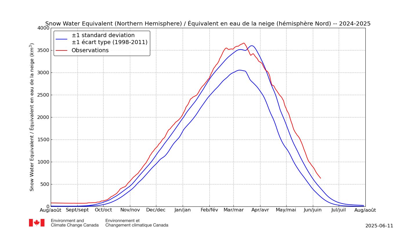
“The oceans of the NH now have a strong warming trend that is producing increased snow extent and new snowfall records are a common occurrence.”
Total BS
These graphs show a time series (updated daily) of the current amount of water stored by the seasonal snowpack (in cubic kilometers) in the Northern Hemisphere’s land areas (excluding Greenland). Let’s return our attention to the snowfall in May.
Red areas on the map show where the surface of the ice is darker than normal, while the blue areas indicate where the surface of the ice is lighter than normal. The map is shown as deviation from the average, i.e. the average of the albedo measured during the period 2000-2009 has been subtracted.

Thanks Rick. Interesting read.
Good correlation is indicated by a linear fit not a parabola or unspecified “polynomial”.
So what was your polynomial, why/how did you select it and what such non-linear “correlation” mean? That looks like some creative statistical methods.