From Dr. Roy Spencer’s Global Warming Blog
September 4th, 2023 by Roy W. Spencer, Ph. D.
The Version 6 global average lower tropospheric temperature (LT) anomaly for August 2023 was +0.69 deg. C departure from the 1991-2020 mean. This is a little above the July 2023 anomaly of +0.64 deg. C.

The linear warming trend since January, 1979 now stands at +0.14 C/decade (+0.12 C/decade over the global-averaged oceans, and +0.19 C/decade over global-averaged land).
Various regional LT departures from the 30-year (1991-2020) average for the last 20 months are:
| YEAR | MO | GLOBE | NHEM. | SHEM. | TROPIC | USA48 | ARCTIC | AUST |
| 2022 | Jan | +0.03 | +0.06 | -0.00 | -0.23 | -0.12 | +0.68 | +0.10 |
| 2022 | Feb | -0.00 | +0.01 | -0.01 | -0.24 | -0.04 | -0.30 | -0.50 |
| 2022 | Mar | +0.15 | +0.28 | +0.03 | -0.07 | +0.22 | +0.74 | +0.02 |
| 2022 | Apr | +0.27 | +0.35 | +0.18 | -0.04 | -0.25 | +0.45 | +0.61 |
| 2022 | May | +0.17 | +0.25 | +0.10 | +0.01 | +0.60 | +0.23 | +0.20 |
| 2022 | Jun | +0.06 | +0.08 | +0.05 | -0.36 | +0.46 | +0.33 | +0.11 |
| 2022 | Jul | +0.36 | +0.37 | +0.35 | +0.13 | +0.84 | +0.56 | +0.65 |
| 2022 | Aug | +0.28 | +0.32 | +0.24 | -0.03 | +0.60 | +0.50 | -0.00 |
| 2022 | Sep | +0.24 | +0.43 | +0.06 | +0.03 | +0.88 | +0.69 | -0.28 |
| 2022 | Oct | +0.32 | +0.43 | +0.21 | +0.04 | +0.16 | +0.93 | +0.04 |
| 2022 | Nov | +0.17 | +0.21 | +0.13 | -0.16 | -0.51 | +0.51 | -0.56 |
| 2022 | Dec | +0.05 | +0.13 | -0.03 | -0.35 | -0.21 | +0.80 | -0.38 |
| 2023 | Jan | -0.04 | +0.05 | -0.14 | -0.38 | +0.12 | -0.12 | -0.50 |
| 2023 | Feb | +0.08 | +0.17 | 0.00 | -0.11 | +0.68 | -0.24 | -0.12 |
| 2023 | Mar | +0.20 | +0.24 | +0.16 | -0.13 | -1.44 | +0.17 | +0.40 |
| 2023 | Apr | +0.18 | +0.11 | +0.25 | -0.03 | -0.38 | +0.53 | +0.21 |
| 2023 | May | +0.37 | +0.30 | +0.44 | +0.39 | +0.57 | +0.66 | -0.09 |
| 2023 | June | +0.38 | +0.47 | +0.29 | +0.55 | -0.35 | +0.45 | +0.06 |
| 2023 | July | +0.64 | +0.73 | +0.56 | +0.87 | +0.53 | +0.91 | +1.43 |
| 2023 | Aug | +0.69 | +0.88 | +0.51 | +0.86 | +0.94 | +1.54 | +1.25 |
The full UAH Global Temperature Report, along with the LT global gridpoint anomaly image for August, 2023 and a more detailed analysis by John Christy of the unusual July conditions, should be available within the next several days here.
Lower Troposphere:
http://vortex.nsstc.uah.edu/data/msu/v6.0/tlt/uahncdc_lt_6.0.txt
Mid-Troposphere:
http://vortex.nsstc.uah.edu/data/msu/v6.0/tmt/uahncdc_mt_6.0.txt
Tropopause:
http://vortex.nsstc.uah.edu/data/msu/v6.0/ttp/uahncdc_tp_6.0.txt
Lower Stratosphere:
http://vortex.nsstc.uah.edu/data/msu/v6.0/tls/uahncdc_ls_6.0.txt
If the next four months average anomalies of .54 degrees C, 2023 will pip out by one hundredth degree the Super El Nino year of 2016 for warmest in the satellite record, ie since 1979.
This could happen, as the combined effects of a strengthening El Nino, the 2022 submarine Tongan eruption and cleaner ship bunker fuel continue to affect global weather. Obviously, CO2 increasing at the same rate as since 1979 is not responsible for suddenly increased atmospheric warmth or decreased Antarctic ice.
However, the cooling trend since Feb. 2016 is at risk.
The climate system really does not want to meet anyone’s expectations.
A rapid rise is usually offset by a rapid fall after a while.
The chart still looks like we are at or near a natural warming peak but the degree of irregularity is surprising.
UAH TLT lags ENSO by 4-5 months. The 0.69 C anomaly corresponds with an ONI of -0.1 or 0.2 depending on whether it is 4 or 5 months. If the typical ENSO lag holds in this case then we are only at the ENSO-neutral level right now. I would not eliminate the possibility that higher values will occur within the next 12 months considering the August ENSO value came in at 1.3 with July ONI at 1.1.
I wonder if the temp level after the El Nino is over will be about .2°C above the ~2000-2015 level, which in turn was about .2°C above the previous period.
Rinse and repeat.
https://imgur.com/ecl8wyD
I don’t know man. This one is different. All of this heat is coming from somewhere.
Maybe volcano belching H2O and ocean dumping heat?
The Sun supplies 99+ percent of the heat. Radioactive decay is the rest.
This is as high as it will go. 2016 peak will not be topped.
We’ll see. I can’t say how long the Tongan effect will persist, but the fuel switch could last a while, however minor.
Last month you said the downtrend from 2016 will remain intact. Are you still confident in that prediction?
All analysis must include that the Earth is still in the warming trend that represents rising out of the Little Ice Age.
There does seem to be evidence the Earth has ever spent much time with stable unchanging temperatures over decades and centuries
Almost like some inviolable rule of complex systems in motion, there is always either a warming or cooling phase in play.
I think of spinning tops, or planets, necessarily precessing on their axes. So our climate system “precessing” around its very long term equilibrium——long term meaning a billion or so years.
In a generally warming environment, of course “new” records for high temperatures are to be expected. The breathless terror these “records” generate in the climate alarmist crowd is amusing in light of climate reality.
Chicken Little and Henny Penny reign supreme in the media world.
TempLS has a similar result for August global surface temperature; about 0.05C higher than July, and about 0.24C higher than any previous August. The mean for year to date is now 0.05C higher than 2016, which had its warm months early in the year.
July and August’s abruptly higher temperatures clearly have nothing whatsoever to do with man-made “climate change”. As of yesterday, Arctic sea ice was right on the average for that date of the decade 2011-20. Last year and 2021 were higher, so this decade is setting up to be icier than the prior decade, despite continually rising CO2, including during the plandemic-driven global deindustrialization of 2020-22.
And what about the long term trend of 0.14 degrees per decade? Is that also unrelated to the rising CO2 levels?
What is “long term” in climate science? The run-up from the little ice age well into the 20th century was not CO2 forced and was much longer term than the satellite record.
Yes. Rising CO2 is mainly the result of natural warming since the end of the LIA c. 170 years ago.
How do you figure that Milo ? If the SST warmed a degree that would only be 12 ppm increase in CO2 due to SST. Meanwhile the increase from 280 ppm to 410 ppm is about half of the amount of CO2 emitted by humans burning stuff. So other phenomena must have absorbed the other half.
So, CO2 causes some warming, which causes an upward temperature trend over a long time, barely discernible against natural variability, that should have an exponential decay ending at about 3C of of global warming by the time we have burnt all our fossil fuel reserves (about 3200 ppm CO2).
Except, well before that (roughly about 800ppm), the finding cost of more fossil fuels will cause nuclear and synthetic or biofuels to be relatively economical (but likely quite expensive for the average person barring some sort of liquid fuel synthesis breakthrough) and the problem (if one assumes the CO2 is a problem) will go away on its own.
DM,
Surely it is time to destroy that 12 ppm calculation calculation which, among others, came from Ferdinand Engelbeen.
The amount of CO2 gas released into the air from the heating of ocean water might or might not follow Henry’s Law.
If it followed that Law, then the weight of gas would relate to the weight of heated water.That amount is not known, adequately or at all, because we lack temperature profiles with depth over all of the oceans. We can only make assumptions about thermocline depths etc.
The picture is one of continuous mixing of water at a rate over time that is not adequately known. In some models, the rate at which charged water is brought to the surface to release gas, is not known.
Second, many chemical reactions increase their rate with heat. If there are biological or inorganic reactions at work to produce CO2 in the oceans, these will affect the relationship apart from Henry’s Law, which starts with a fixed, closed volume in the lab experiments.
Third, the constants in the Henry’s Law equation are derived from small, controlled laboratory experiments where neither the mixing effect nor the background chemical gas production system (if any) will operate.
Apart from that, the laboratory system is not in a vessel with hot, moving plates at its base, spreading and spewing heat and almost always having significant CO2 emission from underwater volcanos, magnitude completely unknown.
It is quite dangerous to use the logic you wrote.
….
BTW, it is also dangerous to assume that future nuclear will be expensive. Our construction cost is currently artificially elevated from past actions of inhappy agitators. Needs must, the price might drop a lot when synthetic concerns are shoved aside. I think that costs in Korea and China are closer to the future costs that we can expect. For some extra material see this: Geoff S
https://wattsupwiththat.com/2023/07/18/corruption-of-science-by-money-and-power/
You should have some faith in Henry’s Law and when people claim more CO2 than Henry’s Law suggests, be skeptical of those claims. The amount of water vapor in the air above the ocean corresponds pretty well to Clausius-Clapeyron when one makes an educated guess of what the relative humidity could be (for mixed vertical air transport). Also, CO2 is well mixed in the atmosphere, so one should expect Henry’s Law to be approximately true as well.
And I never said anything about future nuclear being expensive, my point is that future liquid fuels will be expensive because the days of it being pumped out of the ground nearly for free at accessible locations are coming to an end, decade by decade.
That is demonstrably false and discredits us skeptics. The increase can’t be occurring naturally when CO2 isn’t going up at least as much as we’re emitting.
The annual increase of CO2 in the atmosphere is only about half the CO2 emitted by fossil fuel burning.
In fact natural fluxes are net absorbing CO2. (Which is why the earth is greening and agriculture is booming). Fossil fuel burning and cement production are slightly increasing CO2 concentration in the atmosphere (it’s gone from 0.028% to 0.043%).
It’s all good. CO2 is LIFE!
There’s NO CLIMATE EMERGENCY!
You mean the zero trend apart from El Ninos?
Less tropical cloud.
strong sun still..
I’m not sure why someone would downvote you for posting facts. The Wattage increase in TSI is about 1/3 of what is expected from “greenhouse forcing” which is just better insulation of the energy that already exists in the system, whereas the TSI increase means the whole system has more energy to play with and to reach a new equilibrium.
An increase in TSI of 1.1 W/m2 is equivalent to a radiative forcing of about 0.2 W/m2.
bdgwx,
“I.G. Enting, inEncyclopedia of the Anthropocene, 2018
Radiative ForcingRadiative forcing is the change in the net, downward minus upward, radiative flux (expressed in W m− 2) at the tropopause or top of atmosphere due to a change in an external driver of climate change such as a change in the concentration of carbon dioxide or the output of the Sun.”
So what you are saying seems to be incorrect…
1.1 W/m2 * 0.7 / 4 = 0.2 W/m2
Where’s the mistake?
TSI wasn’t measured prior to the 1980s. That graph is from a model in which scientists introduced a rising trend for which there is no evidence. According to sunspots, solar activity is as low as in the 1900s.
Natalia Krivova and Judith Lean explain it in a 2018 publication:
https://arxiv.org/ftp/arxiv/papers/1601/1601.05397.pdf
As we continue to come out of the Little Ice Age – the world has been warming since about 1700 or earlier – hopefully back up to the warmer levels of the early Roman Empire period, or of the even warmer Minoan period, the warming oceans will release CO2, reaching a new equilibrium with the atmosphere and the biosphere of both land and sea. That’s why, even though humans make more and more CO2 every year, the planet absorbs about half of that, even though that half is larger this year than last year or the year. The biosphere has a lag time in growing in relation to the extra CO2 available. Once human CO2 emissions level off once the population levels off and once everyone reaches the same level of prosperity, we’ll see total CO2 levels continue to grow anyway as the biosphere expands, if the warming continues too.
Roughly and ‘by back of an envelope eyeballing” temperature reconstructions, it seems there was a peak in temps AD100 and AD1100 and troughs (years without summers and economic collapse) roughly AD540 and AD1650 – unfortunately the Minoan Warm period and the bronze age collapse don’t fit the timeframe – but anyways, all other things being equal the natural warming we’re experiencing now would seem to reach a peak in AD2100. But that’s just following the reconstruction graphs – we don’t know why there is this roughly 1000 year cycle, it doesn’t have anything to do with the know orbital variations.
“back of an envelope eyeballing”. Now there is a good way to do science. Not to mention that it depends strongly on what reconstruction you use. Neither the PAGES 12K reconstruction nor Marcott et al.’s reconstrcuction show what you claim to see. Have a look at:
https://content.csbs.utah.edu/~mli/Economics%207004/Marcott_Global%20Temperature%20Reconstructed.pdf
or
https://www.realclimate.org/index.php/archives/2013/09/paleoclimate-the-end-of-the-holocene/
Marcott got pings for scientific malpractice.
Pages2K is a far-left propaganda collaboration aimed at a fake attempt to shore up the AGW scam.
PCman999,
Recovery from the LIA seems a logical matter, but it helps greatly if one also mentions the mechanism by which the temperature has been increased. Is it, for example, from more incoming solar short wave, from extra CO2 in the air, from increased volcanism, from various effects of cloud changes, or what?
Geoff S
Whatever is causing it is cyclical:
https://149366104.v2.pressablecdn.com/wp-content/uploads/2022/06/1850THad-
1654131568.5335.jpg
That’s odd. I can’t get that url to post properly.
You have to copy and paste the whole url to get it to work.
It shows that there were three periods since the Little Ice Age ended where there were periods of warming that were equal in magnitude to the warming of the present day.
It warms for a few decades and then it cools for a few decades and has done so since the 1880’s.
Let me try adding this to the WUWT database.
It MAY be related Izaak. Personally I think that there is an effect. BUT—it’s a minor BENEFICIAL effect. The better question is why you think that a slightly milder climate is a crisis?
If there are any negative effects, we just need to use some of the vast increases in wealth that society can expect in the coming decades to adapt to whatever change comes our way.
What evidence do you have that another 1.1°C rise in temperature by 2100 is going to do anything but increase arable land area and extend growing seasons?
Warmer is better. More CO2 More Life. There is NO CLIMATE EMERGENCY!
The IPCC said the trend should be 0.4 degrees per decade for the measured increase in CO2 levels, with a possible range of 0.25 to 0.65 degrees/decade. The long term trend being so far below the minimum shows that either the assumption of CO2 as the driver of warming was incorrect or the effect of CO2 was so vastly overstated there is no long term concern.
Empirical ECS is 1.7 not 3+
There is NO CLIMATE EMERGENCY!
Yes
LOL, there were long periods of time of no warming in between El-Nino’s which is a step-up warming event in temperature data which indicate that CO2 isn’t driving the trend.
When the trend is trivial, in the end the driver whatever it is must also be weak and offset by negative feedbacks.
I see ENSO as a storage-discharge cycle. It is to be expected that temperatures level off or even decline while energy is stored in the ocean during La Niña. Then when it discharges during El Niño, atmospheric temperatures rise. A continuously rising CO2 concentration generates an increasing LW flux but it’s a complex system. Temperature responds in fits and starts.
The even longer geological history shows that warming and cooling are totally out of synch with CO2. Ergo, CO2 has no effect on climate.
Past CO2 changes were caused by geological and biological process. Man has manages to add 35% CO2 to the atmosphere in only about a century. This doesn’t seem to have done any harm so far, but it’s worth keeping an eye out for what effect on climate it might have. Its also worth keeping an eye out that the opportunists of the world don’t use increased CO2 as a money grubbing opportunity.
I wouldn’t suggest the jump in the last couple of months was due directly to CO2. There’s clearly something very unusual happening, and I doubt anyone knows for sure why.
But the linear rate of warming over the course of the UAH record, about 0.6°C over the last 44 years, is an underlying cause of any record. Whatever caused the recent spike is doing it on top of an already warmer planet.
But the rise in CO2 is largely due to the natural warming coming out of the Little Ice Age, coldest interval of the Holocene, ie past 11,400 years.
https://news.yahoo.com/ozone-hole-above-antarctica-opened-100003567.html
It always opens when it’s dark down there. I think you need the Sun’s rays to blast O2 so that there are free O to join up with O2 to make O3
Bellman:
For the cause of the recent temp. spike read:
“Definitive proof that CO2 does not cause global warming” An update.
https://doi.org/10.30574/wjarr.2023.19.2.1660
The recent spike, like the last spike in 2016 and the one in 1997-8 is due to the El Nino, which has been documented for hundreds of years. If it’s man made, you’ll have to forgive the Conquistadors for destroying the Inca temples and ending the live human sacrifices.
Notice how flat temps are (they go up and they come down and so average out) between El Ninos. The only time there’s the “CO2 signature ” is the 1979-1997 period where the rising trend is clear visible even with the oscillations – though that increase was more likely from pollution reduction than the little bit of CO2 increase, since that started in the early seventies, whereas CO2 production has been increasing for a couple hundred years and never seemed to affect temperature then.
Dr Spencer himself said in the July UAH update that it’s too early for the current El Nino to be influencing global lower stratospheric temperatures. We still have that to look forward to.
“global lower stratospheric temperatures.”
How the **** is that relevant, clown !
“The recent spike, like the last spike in 2016 and the one in 1997-8 is due to the El Nino…”
This is claimed a lot, but it makes no sense to me based on the actual figures. By this time in 1997 or 2015 ENSO was well into red territory (values of over 1.0) and had been positive for some time. Yet the peaks wouldn’t be reached until the following year. This year the June-July period is the first to be even slightly positive.
If the last few months have been in response to the current predicted El Niño, it:s behaving in a way that is very different to what we have seen before. Maybe the accumulated ocean heat has caused some fundamental change in the nature of the ENSO cycle, which could be worrying. But for now I’m just going to assume we don’t know what is happening.
“There’s clearly something very unusual happening, and I doubt anyone knows for sure why.”
There’s something we can agree on.
Tom Abbott:
“I doubt that anyone knows for why”
You must have missed my earlier post:
https://doi.org/10.30574/wjarr.2023.19.2.1660
Nick,
Your specialty, mathematics.
Is a difference of 0.05 deg C statistically significant?
Or, to pose it another way, are 2 of these monthly temperature anomalies able to be distinguised if they are 0.05 deg C different, or are we seeing noise?
Geoff S
It’s close to significant for the full year. But it will be higher by December.
The trend is highly significant.
People like to confuse statistical significance with didn’t happen. Any hot day isn’t statistically significant. But it is still hot.
“But it will be higher by December.”
Nick is playing with his crystal balls again !
No crystal ball required. The El Nino’s effect isn’t even being felt yet in UAH.
How would know ?
You have never been correct with one statement you have ever made.
You are a classic climate alarmist BSer.
Roy Spencer, the guy who makes UAH, says so.
So he said for July. What about August?
Roy has been unequivocal that UAH TLT lags ENSO by 4-5 months. The 4 and 5 month ONI values are 0.2 and -0.1 respectively. UAH still hasn’t responded to the El Nino. It has, however, responded to the transition from La Nina to neutral. Unless the ENSO correlation has suddenly broken down then we haven’t seen the peak in UAH TLT yet.
LOL 🙂
I’m cold. 65F and windy with stratus. What does this mean Holy Nick?
I’d say not noise, but the predicted effect of a rare volcanic event, plus switch in ship fuel.
What is the uncertainty envelope for those numbers?
This is a pretty mechanical response. Did you ask for the uncertainty of Roy’s UAH numbers?
Do you REALLY think that no one noticed that you didn’t answer the question? The uncertainty of UAH is irrelevant to the question posed directly to you.
It’s obvious that you either don’t know the answer or don’t want to offer the answer for some reason.
Either way, it puts a load of doubt on everything you post since no one can judge whether the ΔT is large enough to overcome the uncertainty.
So is there a load of doubt on Roy’s post?
It’s not doubt, it’s uncertainty that no one ever discusses. Even you treat the ΔT as an exact number that has no variance associated with it. People who work with real physical measurements never do this.
When you see a measurement whose uncertainty is 0.2, quoted to the hundredths digit, alarm bells go off. If the uncertainty is quoted to two digits, like 0.20, one can believe the uncertainty has been evaluated to the hundredths digit.
Too many mathematicians have been trained that numbers are just numbers to be manipulated however you wish.
To physical scientists and engineers, numbers are not just numbers. They portray and represent physical measurements that have rules to be followed when using them. No measurement is ever considered exact, there is always uncertainty based upon Type A and Type B uncertainties and resolution is one of the things that causes uncertainty.
Satellites are about ±0.2 C [1][2]. Traditional surface are about ±0.05 C [3][4][5]
Not only NO, but HELL NO! Traditional surface temperature measurement devices have uncertainties in the +/- 0.3C to +/- 1.0C range.
No matter how you try to rationalize it to yourself the surface average temperature simply can’t have an uncertainty less than that.
You continue to push two memes no matter how often you are shown they are wrong.
Surface measurement devices always, ALWAYS, have systematic uncertainty. It can’t be identified through statistical methods and therefore cannot be cancelled out in any way, shape, or form.
q = Σx_i/n is the AVERAGE VALUE of a series of temperature measurements. When you find the uncertainty associated with that formula you are finding the AVERAGE UNCERTAINTY, not the uncertainty of the average.
See the attached picture. The average uncertainty is 2.2. The total uncertainty is 13. They are *NOT* the same. All you do when you find the average uncertainty is take the total uncertainty and spread it evenly across all individual members of the data set – you still wind up with the same total uncertainty.
The proof of the pudding is that you will not list out the variances of the temperature data sets, beginning with the individual daily mid-range values and ending with the final global average. Neither will anyone else trying to advance the CAGW agenda. Averaging doesn’t lower variance. Anomalies don’t lower variance.
The daily temperature has a variance of Tmax – Tmin. When you do (Tmax+Tmin)/2 you don’t lower that variance, it remains. The result should be written as [ mean = m, variance = d] where d is the diurnal range for that day.
When you combine Day1 random variable with Day 2 random variable you get:
m_t = m1 + m2, d_t = d1 + d2 (variances add when adding random variables)
This only involves the stated values of the temperatures and doesn’t even consider the measurement uncertainties associated with the stated values of the temperature.
Now come back and tell us that all measurement uncertainty is random, Gaussian, and cancels plus variances can be ignored.
And if all the rounds go through the same hole, the standard deviation is ZERO, which means the SEM is ZERO, yet somehow all the rounds are still off-bullseye.
Go figure.
Which as I explained to you in another comment thread, is a good illustration of the usefulness of the SEM. If you have a very small (or even zero) SEM, you know that any difference between the sample average and the expected average (in this case a bullseye) can not be down to chance. You’ve just demonstrated, using SEM that there is a systematic error in your gun.
You just demonstrated your abject ignorance, again.
In real metrology true values are UNKNOWN.
bgwxyz trots out his milli-Kelvin “uncertainties” again, nothing new under the sun.
The real problem is using the variance in the anomaliy distribution to represent the inherent uncertainty.
You are averaging small numbers and will end up with small variances.
Anomalies are calculated by subtracting absolute temperatures. The uncertainty should carry the variance of those absolute temperatures, and not the variance of the anomalies.
I’m sure many, many people here that are familiar with measuring instruments also know that it is impossible to increase the resolution of measurement by averaging.
If I measure something to the nearest 1/8 of an inch. I cannot, no way, average 1000 measurements and get an answer that has a smaller resolution. Not one chemistry lab, physics lab, or engineering class/lab would let a student do this.
“If I measure something to the nearest 1/8 of an inch. I cannot, no way, average 1000 measurements and get an answer that has a smaller resolution.”
I keep demonstrating this is not true if you are taking the average of things of different size. You could easily test it for yourself if you weren’t afraid of proving every chemistry lab, physics lab, or engineering class/lab wrong.
Just take 1000 random bits of wood, all of different sizes. Measure each with a very precise instrument, and then again with your 1/8 inch ruler. Compare the averages. Is your low resolution average closer to the precise average, than 1/8 inch.
I can easily test this using R. I’ve just generated 1000 random rods, from a random uniform distribution going from 10″ to 14″.
The precise average of these 1000 rods is 11.915″.
Then I “measure” each with your low resolution ruler – that is I round each size to the nearest 1/8″, i.e 0.125″. By your logic the resolution of the average of the low resolution measurements should be 1/8″. In fact the average is 11.914″.
The precise difference between the two was 0.00118″. This to my mind suggests the resolution is better than 0.125″.
No, you keep generating clownish noise to obscure your trendology non-physical nonsense.
Your lack of training in the physical sciences is showing again. Why do you insist on speaking of things you know nothing about?
Science uses the rules of significant figures. When you add/subtract/multiply/divide your final answer should have no more significant digits than the element with the least significant figures.
Your supposed simulation went from 3 decimal places to 5 decimal places. How did you do that?
All you know is statistics world where the number of digits on your calculator determines the final answer. The more digits it displays the better resolution you have.
That isn’t how physical science works.
(p.s. .914 / .125 is not an even number. You didn’t even get the number of 1/8″ increments correct in your average)
The magic of averaging?
Magical thinking, certainly.
And as usual, rather than addressing the argument, or providing evidence against it – there’s the usual ad hominem and arguments from tradition. “It’s what we were taught at school, and you don’t understand anything.”
It’s as if you keep insisting man will never fly, I keep pointing to planes, and you just say they are impossible and say I need to learn why they are impossible before I’ll understand. It’s religious dogma.
“Science uses the rules of significant figures”
You know I don’t share that faith – quoting from the holy scriptures is futile.
“When you add/subtract/multiply/divide your final answer should have no more significant digits than the element with the least significant figures.”
You don’t even understand your own dogma. The “rules” are when you multiply and divide the result has the same number of significant figures as the element with he least, but when add or subtract it’s the element with the fewest decimal places that determines the resulting number of decimal places.
As I’ve demonstrated before, just following these rules will allow you to have more significant figures in an average than you would like. Add 100 figures to 1 decimal place, the total will still be to 1 decimal place. Now divide by 100 and the answer would be quoted to 3 decimal places.
Which is why to justify your claim there has to be an extra special rule that only applies to averages.
“Your supposed simulation went from 3 decimal places to 5 decimal places. How did you do that?”
Oh I’m a naughty heretic – I quoted to as many figures as a I wanted to demonstrate the point. But if it offends your sensibilities
“The more digits it displays the better resolution you have.”
No. The closer the calculated average was tot he true average, the better the resolution. Really this shouldn’t be hard even for. I created a set of random numbers known to as many decimal places as you could wish and calculated their average. Then I reduced the resolution of the figures by rounding to 1/8″ (0.125″), and according to your logic the resolution of the average should have been 1/8″, yet it was almost identical to the true average, differing only by 0.001″. This demonstrates that the resolution of an average can be higher than that of the individual measurements.
“p.s. .914 / .125 is not an even number.”
Huh?
Nice screed, LoopholeMan.
“You know I don’t share that faith – quoting from the holy scriptures is futile.”
We *all* know you think physical science is totally wrong in using significant figures. It stems from you having *NO* STEM background at all. You’ve apparently never, ever had a high level physical science lab course (i.e. physics, chemistry, engineering, etc) let alone any real world experience in actually measuring something that impacts human life and well-being.
“As I’ve demonstrated before, just following these rules will allow you to have more significant figures in an average than you would like.”
NO, they will not. You misapply them every single time. Jim already pointed out to you the reason you can’t is right there in Taylor’s book – which you absolutely refuse to study.
” Now divide by 100 and the answer would be quoted to 3 decimal places.”
Nope! You can’t even count significant figures. 100 has *ONE* significant figure. If the measurements are good to one significant figure then dividing by a number with one significant figure won’t change anything.
If the 100 measurements are good only to the tenths digit (i.e. uncertainty is +/- 0.1) then the answer is good only to the tenths digit. Same for their average.
You are trying to somehow rationalize that you can take an average and it will increase resolution. Climate science may believe that, *YOU* may believe that, but in the real world NO ONE believes that.
“We *all* know you think physical science is totally wrong in using significant figures.”
Only if it using these simplified rules to work out uncertainty.
“Nope! You can’t even count significant figures. 100 has *ONE* significant figure. ”
And there you go, demonstrating you don;t even understand the dogma you force on others. 100 is an exact number, exact numbers have infinite significant figures.
http://www.ruf.rice.edu/~kekule/SignificantFigureRules1.pdf
http://www.astro.yale.edu/astro120/SigFig.pdf
“You are trying to somehow rationalize that you can take an average and it will increase resolution.”
Yes, that’s exactly what I’ve been trying to tell you. An average can have a better resolution than the measurements that make it up. If you want to persuade me I’m wrong, you need to provide some evidence that is better than simply yelling that it can’t be so.
“Jim already pointed out to you the reason you can’t is right there in Taylor’s book”
He has not done anything of the sort. Taylor does not say that – he explicitly points out that in some exercises you can quote more figures than the individual measurements. All he says is the number of figures has to be the same order as the uncertainty – something I agree with. And he also points out that taking an average reduces the uncertainty.
Maybe on Neptune. Stop sniffing methane.
As usual, you didn’t bother to even read the definitions you cherry-picked!
“Thus, number of apparent significant figures in any exact number can be ignored as a limiting factor in determining the number of significant figures in the result of a calculation.”
I said: “Nope! You can’t even count significant figures. 100 has *ONE* significant figure. If the measurements are good to one significant figure then dividing by a number with one significant figure won’t change anything.”
It simply doesn’t matter if you consider the 100 as having infinite sig digits or one, it doesn’t affect the number of sig digits the answer has.
“If you want to persuade me I’m wrong, you need to provide some evidence that is better than simply yelling that it can’t be so.”
I have. Multiple times. The fact that you can’t read is not *my* problem, it’s yours. Your logic says you can reduce uncertainty to the thousandths digit using a yardstick. It’s nonsense on the face of it. And it is something you have yet to explain. You just ignore it when someone points that simple fact out to you.
“Taylor does not say that – he explicitly points out that in some exercises you can quote more figures than the individual measurements.”
Once again, you have not STUDIED Taylor at all. You continue to just cherry-pick with no understanding of context at all. Taylor covers this in Chapter 2, right at the start of the book! “In high-precision work, uncertainties are sometimes stated with two significant figures, but for our purposes we can state the following rule:
Rule for stating uncertainties:Experimental uncertaintites should almost always be rounded to one significant figure.”
He follows this with Rule 2.9: “The last significant figure in any stated answer should usually be of the same order of magnitude (in the same decimal position) as the uncertainty.”
There is a *reason* why physical science and engineering uses the significant figure rules. You don’t seem to be able to grasp it at all. Instead you just claim that hundreds of years of practice by physical scientists and engineers is wrong because you can calculate out to 8 or 16 digits on your calculator.
The concept has to do with repeatability. If you are publishing experimental results or design calculations what you state for the stated value and for the uncertainty has to be repeatable. Being repeatable applies to averages as well as individual measurements. Taylor states it very well in Chapter 2: “If we measure the acceleration of gravity g, it would be absurd to state a result like 9.82 +/- 0.02385 m/s^2”
My guess is that you don’t have a clue as to why this would be an absurd result. It *is* what *you* might get by averaging the individual uncertainties of the multiple measurements taken during the experiment and ignoring significant figure rules.
I’m not eve going to give you a hint as to why this is an absurd result. You’d just say it’s wrong.
“As usual, you didn’t bother to even read the definitions you cherry-picked!”
You made two statements. I was correcting the first one. Statement 1) A divisor of 100 has 1 significant figure. Statement 2) some waffle about measurements being good to 1 significant figure.
Your first statement is just wrong. Your second is also probably wrong, and irrelevant to the case we were discussing.
Let’s suppose you had 100 measurements, each with a single significant figure. Lets say they were all integers between 1 and 9. How many significant figures does the sum of these 100 figures have? Remember when adding it’s the lowest decimal place that counts, so the sum will have a unit as it’s final significant figure. Obviously the sum has to be between 100 and 900, so has to have 3 significant figures. Now divide by 100, and report to the same number of significant figures as the smallest value, i.e. 3 (3 < infinity). So if say the sum was 518, the average would be written 5.18.
“Taylor covers this in Chapter 2, right at the start of the book! “In high-precision work, uncertainties are sometimes stated with two significant figures, but for our purposes we can state the following rule:”
Which is nothing to do with the point I’m making. Which is if you have a mean of a large number of values measured to the nearest unit, the uncertainty may well be less than a tenth of a unit, in which case you should report the result to the nearest tenth of a unit.
“… because you can calculate out to 8 or 16 digits on your calculator.”
Again, you just demonstrate you didn’t read what I wrote, and are just arguing with the voices in your head.
“Let’s suppose you had 100 measurements, each with a single significant figure. Lets say they were all integers between 1 and 9.”
If these are measurements and you are getting values ranging from 1 to 9 then I would tell you to get a different measuring device!
“Which is nothing to do with the point I’m making.”
The only issue at hand is MEASUREMENTS and MEASUREMENT UNCERTAINTY. Significant figures and measurement uncertainty are concepts to make measurements in the physical sciences and in engineering repeatable and meaningful.
Something which you simply cannot address with any competency at all.
All you want to do is show how many digits your calculator can handle – which is meaningless when it comes to measurements.
“Which is if you have a mean of a large number of values measured to the nearest unit, the uncertainty may well be less than a tenth of a unit, in which case you should report the result to the nearest tenth of a unit.”
If your measurements range from 1 to 9 then the uncertainty is in the units digit – PERIOD.
“If these are measurements and you are getting values ranging from 1 to 9 then I would tell you to get a different measuring device!”
For the hard of thinking, that’s 100 measurements of different things.
“The only issue at hand is MEASUREMENTS and MEASUREMENT UNCERTAINTY. ”
and the point flies over his head again.
“All you want to do is show how many digits your calculator can handle”
A) I am not using a calculator.
B) The measurements are rounded to 1 decimal place, so each have 3 significant figures.
“If your measurements range from 1 to 9 then the uncertainty is in the units digit – PERIOD. ”
Which is why I said the measurements only have one digit. But, following the precious rules allows me to write the average to 3 decimal places.
Ambiguity strikes again. You blokes are using separate lines of argument.
bellman is pretty much correct about the number of decimal places which can be used in reporting averages in the absence of uncertainty. It’s the order of magnitude of the count.
The arithmetic mean is the ratio of the sum over the count.
125/100 is 1.25
1250/1000 is 1.250
1250000/1000000 is 1.250000
Tim is also right about the number of decimal places used with measurements, which always have uncertainties.
A measurement of 1.25 is shorthand for 1.250 +/- 0.005, just as 1.250 is shorthand for 1.2500 +/- 0.0005.
Hopefully some progress can be made once the definitions and topic of discussion are agreed upon.
As to whether the uncertainties should be added directly or in quadrature, or as absolute or relative uncertainties, my Physics and Chemistry lab sessions are too far in the past.
“Ambiguity strikes again. You blokes are using separate lines of argument.”
In more ways than one.
“bellman is pretty much correct about the number of decimal places which can be used in reporting averages in the absence of uncertainty.”
Thanks – though I should say that some rules for significant figures do say that the mean should only be quoted to the same number of places as the measurements. My point is that this seems to be tacked on as a “special” rule, and I’ve never seen justified.
I suspect the problem is that these rules are only intended as an introduction, before proper rules of uncertainty are introduced. They make sense when dealing with averaging the same thing a few times, but are way off when applied to large scale samples of different things.
“A measurement of 1.25 is shorthand for 1.250 +/- 0.005, just as 1.250 is shorthand for 1.2500 +/- 0.0005.”
I don;t disagree that that is a short hand, and in some cases might be a useful one. But I much prefer having an explicit uncertainty range. The more I’ve thought about this convention for problems I see.
From what Tim has said though I think the real problem is we never agree with what an average is. I see it as an abstract description of the mean of a population,. whereas he sees it as representing an actual thing – and if nothing is the same as an average than the average does not exist.
The idea that the average can only be as good as a single measure springs from that, and would make sense if you were talking about a median, rather than a mean.
I kept it to integer values to take measurement uncertainty out of that part of the picture. I was purely looking at the number of significant digits attributable to the order of magnitude of the denominator.
That’s a point I’ve brought up a few times. “Average” is a very vague term, which usually means one of the 3 Ms, and you have to guess which one from context.
Even “mean” is ambiguous, ranging from the commonly accepted “arithmetic mean” or “weighted arithmetic mean” to “expected value”. Without agreeing on defined terms, it’s almost guaranteed that people will talk past each other and become frustrated.
Interesting. My educational background assumes it’s derived from the sample, and to determine whether it’s the mean, median or mode.
Then there’s the question of what the mean means. Again, my background says it’s just one of the measures of centrality of a distribution, and to look for the mode, median, range and variance/SD to characterise the distribution.
“Thanks – though I should say that some rules for significant figures do say that the mean should only be quoted to the same number of places as the measurements. My point is that this seems to be tacked on as a “special” rule, and I’ve never seen justified”
This has been justified to you over and over and over again.
It’s so that others looking at your results don’t assume you were using a measuring device with higher resolution that you were actually using! It has *everything* to do with the repeatability of measurement results.
We remember that your ultimate goal is to justify climate science identifying anomaly differences in the hundredths digit from measurements with uncertainties in the units digit. Thus you claim you can increase measurement resolution, and therefore uncertainty, by averaging.
When confronted you start making up numbers like 100 measurements ranging from 1 through 9 – and then refuse to accept that the range of those values indicate either a broken measurement device or a multi-modal distribution – and in either case the measurement uncertainty is huge, even for the average! You just retreat to the excuse that the SEM is the uncertainty of the average.
A mathematician versus a physical engineer. Measurements of a measurand ARE a description of a physical phenomenon. They are not an abstract notion of a population.
It is why you continually dwell on statistical calculations of how to do the math to achieve a number. It is why you never give examples of physical things to measure and how their physical measurements should be calculated.
To you temperature measurements are abstract numbers and the entire process is finding a number that shows how close the mean can be calculated. The more decimal digits you can calculate, the more accurate you can say the mean is. It is why you want to shoehorn an average of disparate measurements into a functional relationship that can be treated as a real measurement of a real thing. The more you include, the larger “n” becomes and the smaller the SEM becomes. You have reached the goal of a mathematician, you calculated the mean to an exact number.
Engineers and physical scientists deal with physical things. Our goal is to measure the physical properties of a measurand as best we can. It is unethical to reduce measurement uncertainty by just concentrating on how accurately a mean can be calculated while the measurements themselves demonstrate a large variance.
Here is how Dr. Taylor explains it his book in Sections 4.3 & 4.4. He made 10 measurements of a spring constant and obtained a mean of 85.7 ± 2. The uncertainty is the Standard Deviation of the 10 measurements. He says that this uncertainty can be used to characterize SINGLE measurements of other springs with their uncertainty. I suspect this is how NOAA/NWS has determined a ±1 F uncertainty that should be applied for single temperature measurements. Dr. Taylor shows that you can also specify the SEM for the uncertainty in the one spring that has the 10 measurements. As usual, Dr. Taylor makes it plain this only works for the same spring and that it must be stated that if the SEM is used, one must specify that the SEM is being quoted for a single item.
Here is another diamond from a note by Dr. Taylor. If the single measurements of the spring constant of other springs begin to differ substantially from the average of the first spring, one must reevaluate the whole uncertainty. Think about what this means for temperatures with different devices and locations.
Lastly, resolution is important in science. It defines repeatability and what others attempting to duplicate experiments can expect. That is why Standard Deviation is more important that SEM. It informs others of the range of values you measured. An SEM does not provide the ability to know what to expect in measurements. It only defines how accurately you were able to calculate the mean without informing you of the variability of what was actually measured. Think about it, does the mean anomaly value of ΔT provide any information about the range of ΔT’s used to calculate it?
Can you imagine what might happen if bellman was responsible process control in a factory?
Yikes.
“Measurements of a measurand ARE a description of a physical phenomenon. They are not an abstract notion of a population.”
Yet you keep insisting we have to follow the “NIST method” which treats the average monthly temperature as a thing to be measured, and all the daily temperatures as different measurements of that thing.
But as I keep saying – if you don’t want to treat a sample mean as a measurement of the population, stop insisting we have to propagate the measurement uncertainties. If the mean isn’t a measurand, then nothing in the GUM applies to it, and we can just go back to using the accepted statistical results.
“It is why you continually dwell on statistical calculations of how to do the math to achieve a number.”
Because they are a powerful and well researched tool for explaining the real world.
“To you temperature measurements are abstract numbers”
They are not – but that doesn’t mean you can’t use abstract numbers to analyze and them. All numbers are abstract, even the ones you use to measure the length of your rods, it doesn’t mean they cannot describe concrete things.
“The more decimal digits you can calculate, the more accurate you can say the mean is.”
Absolutely not what I’ve said.
“It is why you want to shoehorn an average of disparate measurements into a functional relationship that can be treated as a real measurement of a real thing.”
You still don’t know what functional relationship means.
“You have reached the goal of a mathematician, you calculated the mean to an exact number.”
You really can;t be this dense. The point of estimating a SEM is because you don’t know what the exact average is. It’s telling you how much uncertainty there is in your average.
“Our goal is to measure the physical properties of a measurand as best we can.”
I would hope physical science has better goals than that. Good measurements are important, but the main goal is to figure out what they mean, what questions they raise, and how those questions can be answered – and a lot of that involves statistical reasoning.
“Here is how Dr. Taylor”
And we are into the usual “If Dr Taylor uses statistics for one purpose, that is the only way they can used.”
Who are “we”?
“ if you don’t want to treat a sample mean as a measurement of the population”
You simply can’t get *anything* right, can you? No one is saying the mean of the population is not a measurement of the population.
They are saying that the MEASUREMENT UNCERTAINTY of that mean is *NOT* the SEM. It is the propagated uncertainty from the individual elements.
Again, one more time, once your measurement uncertainty overwhelms the resolution of your measuring device, YOU ARE DONE! If you uncertainty is in the units digit then whatever value you come up with in the millionth digit is useless. It’s within the uncertainty interval and that millionth digit is UNKNOWN.
If you have a frequency counter that displays a value in the Hz digit at 10Mhz but the uncertainty of the counter is 1%, then the value in the Hz position IS UNKNOWN. It is within the uncertainty interval. The uncertainty interval would range from 9.999.990 Hz to 10.000.010 Hz. No matter how many times you measure that approximately 10Mhz signal you can’t increase the resolution to the Hz digit because it is UNKNOWN, each and every time. It doesn’t matter if you can calculate the average out to sixteen decimal places, it doesn’t change the uncertainty or the resolution of measurement.
When you say it would take 10,000 measurements or more for you to refine the reading of your cell phone timer you are speaking of the SEM! How precisely you can calculate the mean.
The problem is what you identified. Your reaction time puts the uncertainty of each and every reading in at least the hundredths digit. The uncertainty of the mean will be in at least the hundredths digit, not in the millionth digit. It simply doesn’t matter how many measurements you take or how many digits you use in calculating the mean, the measurement uncertainty will remain in at least the hundredths digit and, quite possibly, in the tenths or unit digit depending on your reaction time.
The timer resolution being in the hundredths digit doesn’t matter if your reaction time causes the measurement uncertainty to be in the tenths digit. Once the measurement uncertainty interval has covered up the resolution, you are DONE. Trying to extend the measurement resolution beyond the measurement uncertainty interval is a waste of time and resources.
The goal in measurement is not JUST using higher resolution instruments but also more accurate instruments. It doesn’t matter what the resolution of your instrument is if the measurement uncertainty covers up that resolution. Measuring 1.123456789 seconds is useless if your measurement uncertainty is +/- 0.1 seconds.
Climate science makes the same mistake you always make. They ignore the measurement uncertainty and think they can extend resolution from +/- 1.0C to +/- 0.005C merely by averaging. You can’t. Anything past the unit’s digit is UNKNOWN. What climate science is truly doing is trying to guess at the location of a diamond in a fish tank full of milk. That location is UNKNOWN and will always be UNKNOWN. Until they start properly handling the variances of the temperatures anything they come up with is simply not fit for purpose!
And the reaction time will be bias error, that is not constant!
How can this be washed away with averaging?
IT CAN’T.
Yes, that was part of my point. The reaction time will likely have a systematic error that will be left no matter how much averaging you do.
These are all integers, not measurements, therefore there is no measurement uncertainty.
Totally different.
The first half of the comment was purely about the mean, and how it can be expressed. Using integers keeps it in a purer form.
The object of the exercise is to try to get people to at least agree on the terminology so they’re arguing about roughly the same thing.
Yet measurement uncertainty deals with floating-point numbers, significant digits have absolutely no meaning for integers.
“1250000/1000000 is 1.250000″
Without decimal points on both the sum and the divisor, you can’t claim the ratio is 1.250000, i.e. seven significant digits.
I hearken back to the old venerable slide rule. It’s why, at least in engineering, you would always specify numbers as exponents of 10, e.g. 1.25 x 10^6. Easy enough to tell how many significant figures in that. Calculators have made so many people totally unable to properly represent measurements.
Goes back to the old saying: “its within an order of magnitude”.
That’s right, but significant digits do have meaning for means of integers.
They’re an indication of the sample size, at least to the order of magnitude level.
Oh, yes I can!
I counted them, so I know the numbers involved. It is what it is, and that’s all what it is. If the sum was 1250001 instead of 1250000, the result is 1.250001.
It also tells readers that the sample or population size is of the order of magnitude of a million.
If it was 1250000/999999, I wouldn’t be justified in using 1.25000125000, but I would be justified in using 1.250001.
It’s unusual for a sample to be anywhere near this large, so it also tells readers that this is the population statistic.
And none of it is of much use without the other summary statistics needed to characterise the distribution.
No, without decimal points or exponential notation, you cannot assume a number of digits.
Your huge number has to be written as 1250000. or 1.25×10^6.
No, my huge number was 1,250,000, and it came from a population of 1,000,000. Let’s say 1.250,000 cars registered to 1,000,000 people.
The mean cars registered per person is 1.250000.
The numbers I used were a bad example, because they were too round. Let’s have 1.250,108 cars, and stick with an exact 1,000,000 people. The mean is 1.250108. This is valid because of the order of magnitude of the sample size.
As I said in a reply to another comment, reconciling significant digits between counts and measurements is beyond my pay grade.
If your value is used in a software calculation, it will be converted to floating point representation because the ratio is a floating point. So it really doesn’t matter.
And if the long division is done by hand it will have the same value.
It’s just a convenient way of displaying a ratio.
I don’t think you want to get into a competition with me about how far we can wet up the wall as far as computers are concerned 🙂
??
If the division of 1.250,000 by 1,000,000 is done by hand or by calculator firmware or computer software, the result is the same.
Similarly, if the 1.250000 is used in a calculation done by hand, the result should be the same as a calculation performed in firmware or software. It will take longer, and most likely require more checking, which is why we use computers.
What calculations do you plan to use the mean in?
Counting is not measuring using a measuring device. Taylor covers this in Section 3.2.
Counting occurrences of something typically requires it to be done over a time interval. There is no guarantee that the same number of occurrences will happen in a subsequent, equal time period. So his rule is that you use the count, ν (nu), as the average +/- sqrt(ν).
average number of occurrences per time = ν +/- sqrt(ν)
If you are just counting, like the number of glasses in your kitchen cupboard, where no time interval applies, then there shouldn’t be any uncertainty to calculate. But neither does this represent a measurement.
It is measurements that are the issue here, the measurement of temperatures and how they combine to form a global average temperature.
There are so many problems with how climate science does this that the final result is simply not fit for purpose. And no amount of “averaging” or precisely locating the average value can make it so.
Remember, bellman has several evasion tactics he uses. One of them is redirecting the discussion away from the subject at hand.
The issue is *NOT* how you find the average of a series of numbers that have no relationship to measurements – but that is where he wants to take the discussion because he knows we are correct in our assessments of how you do measurements and measurement uncertainty.
“One of them is redirecting the discussion away from the subject at hand.”
Fine words from someone who has spent the last day ignoring the point of my simple demonstration, and instead focusing on how many digits I reported the random numbers to.
Yes, yes, yes. The communication problems seem to involve the correct statistical treatment of measurements.
The rules which apply to discrete values (counts, if you will) get blurred when measurements and uncertainty are involved.
The object of the exercise is to hash out whether temperature differences in the hundredths digit can be determined from temperatures with measurement uncertainty in the units digit or tenths digit.
Climate science says you *can*. bellman is trying to prove that you can. They say you can improve resolution by averaging measurements with uncertainties in the units digit or tenths digit.
The physical scientists and engineers here are saying you can’t. You can’t increase resolution past what you can measure. Calculating an average out to the limits of the calculator is not increasing resolution.
This seems to be the core of the disconnect.
It certainly is possible with discrete values, or at least it looks like it.
But, and this is a big but, it doesn’t really increase the resolution.
The number of significant digits (actually the number of digits to the right of the decimal point) is the order of magnitude of the denominator.
Just like the number of decimal places reported for a measurement represents the resolution of the measuring instrument, the number of decimal places reported for the mean of discrete values represents the order of magnitude of the population or sample size.
Reconciling the two is beyond my pay grade.
All of this is a huge non sequitur for averaging air temperature measurements, which are most certainly not integers.
Measurements are continuous on the number line. A measurement can have any value along the number line. A discrete value is one where there is no immediately adjacent area on the number line that it can take on.
Typically discrete numbers are considered to be integers but I don’t think that is a requirement. If 10.1 and 10.2 are two possible values for the object but there can’t be any values between those two points then they are discrete values. (perhaps it’s just a matter of scaling?)
Bellman and climate science try to make all measurements into basically discrete numbers, that way they don’t have to worry about the possible vales on the number line that the measurement could also be.
“Measurements are continuous on the number line.”
Not if you are measuring things to any number of significant digits, they are not.
“Bellman and climate science try to make all measurements into basically discrete numbers, that way they don’t have to worry about the possible vales on the number line that the measurement could also be.”
Of course not. The assumption is that the thing being measured can have any value, i.e.is continuous, but any measurement that involves rounding will give you a discrete value. However, the uncertainty will be a continuous value, all calculations are based on them being continuous.
Specifying an uncertainty as a standard deviation, or as an expanded uncertainty interval generally implies that the measurand could take any value within the range.
“Not if you are measuring things to any number of significant digits, they are not.”
Once again you totally miss the point. Measurements are a CONTINUOUS variable. The value can be *anything*. There is no separation between one value and the next. With a discrete variable it can only take on certain values. There is always a gap between one value and the next.
You are simply unable to understand the real world at all. Resolution is only how far down you can measure it. It is not a determinative factor as to whether it is continuous or not.
“The assumption is that the thing being measured can have any value, i.e.is continuous, but any measurement that involves rounding will give you a discrete value”
NO! It doesn’t become a discrete value. Look at the GUM one more time! ““the dispersion of the values that could reasonably be attributed to the measurand”
There is absolutely nothing that keeps the measurement from taking on ANY value that can be attributed to the measurand. You just keep on ignoring what the uncertainty interval is for! The stated value is just that, a stated value, it’s the dial indication if you will. But the uncertainty interval gives you an indication of what the stated value *could* be if the measurement is repeated. Those possible values are CONTINUOUS on the number line.
“Specifying an uncertainty as a standard deviation, or as an expanded uncertainty interval generally implies that the measurand could take any value within the range.”
And here is your cognitive dissonance at its finest. A measurement is a discrete value but it can take on any value within the range.
Just more waffling and shooting from the hip.
Yep!
Or what about rounding? That standard method of converting air temperature F to C comes to mind.
Yes, they are different animals.
That wasn’t about measurements, it was about how means of discrete integer values can validly be decimals, to a certain number of decimal places.
Without the metrology domain knowledge, it is easy to bring those integer rules into the field of measured values.
By the same token, it is easy to view everything as measured values with implicit or explicit resolution limits.
This is all about measurements; without them, you know nothing,
I *still* can’t find a statistics textbook that has any examples where the data values are given as “stated value +/- uncertainty”. They all assume the stated values are 100% accurate and how precisely you can calculate the population mean is the “uncertainty of the mean”.
That simply isn’t real world. It’s why engineers and physical scientists learn early on in lab work that you *have* to work with measurement uncertainty. You just can’t assume all stated values are 100% accurate.
bellman says his cell phone stop watch only reads in the hundredths digit and he would need many, many measurements to get to the microsecond. He can’t seem to understand that when he says this he is talking about the SEM, i.e. how precisely he can locate the population average. It is *NOT* the measurement uncertainty of the average which would likely be in the tenths digit if he has *very* good reaction times.
If your uncertainty is in the tenths digit then the value in any decimal point further out is UNKNOWN. It doesn’t matter how many digits you carry out the SEM calculation, once you go past the measurement uncertainty digit it’s all UNKNOWN, including the population average!
I have the classic Snedcor & Cochoran text and it certainly doesn’t. The closest it comes is when it deals with linear regression when the “x axis has error”, if I remember right.
That’s because they’re statistics textbooks, not metrology textbooks.
Most statistics work is done with “things” rather than measurements, and it’s usually the number of “things”.
That’s the basis on which more specialised areas build. Metrology is one of those specialised areas.
Would it be useful to at least touch on the additional complexities introduced by measurement uncertainty? Yes, certainly. But it would only be a light touch, or statisticians would be metrologists.
This is not a fight between statistics and metrology: bellman apparently believes it is possible to extract information from nothing. Where in statistics is this outlandish claim made?
“from nothing”? I think you can extract information from large amounts of measurements – the larger the better,
The SEM is *NOT* a statistical descriptor of a population distribution. When you try to use it as one then you *are* trying to extract information from nothing.
https://pubmed.ncbi.nlm.nih.gov/12644429/
“Background: In biomedical research papers, authors often use descriptive statistics to describe the study sample. The standard deviation (SD) describes the variability between individuals in a sample; the standard error of the mean (SEM) describes the uncertainty of how the sample mean represents the population mean. Authors often, inappropriately, report the SEM when describing the sample. As the SEM is always less than the SD, it misleads the reader into underestimating the variability between individuals within the study sample.”
https://pubmed.ncbi.nlm.nih.gov/24767642/
“The study was designed to investigate the frequency of misusing standard error of the mean (SEM) in place of standard deviation (SD) to describe study samples in four selected journals published in 2011. Citation counts of articles and the relationship between the misuse rate and impact factor, immediacy index, or cited half-life were also evaluated.”
The SEM tells you literally NOTHNG about the population distribution. It is *NOT* a descriptive statistic for the population. The SEM is only an indicator of how closely the sample represents the population and even then it is subject to restrictions in its use.
Your focus on the SEM as a statistical descriptor of the population is wrong-headed, even for a statistician. The fact that you won’t admit that is telling.
I see the phrase of the day is “statistical descriptor “.
Correct,the standard error of an the mean is not s statistical descriptor. That’s why it’s better to not call it a standard deviation.
Why you would that mean the SEM is created out of nothing, I’s something only you could explain.
“Your focus on the SEM as a statistical descriptor of the population is wrong-headed, even for a statistician. ”
And nobody should be doing that. The sample mean is a best estimate for the population mean. The SEM is an indicator of how good that estimate is. You might not have a use for that information or understand it, but it is widely used throughout the sciences.
Have you gotten past the Introduction for your paper yet?
The standard error of the sample means – the *real* definition of the SEM – *is* a standard deviation. It is the spread of the sample means. It’s just not the standard deviation of the population or the measurement uncertainty of the population.
The SEM tells you *NOTHING* about the population since it is not a statistical descriptor of the population. Anything *YOU* or climate science uses it for in relation to the population of temperature measurements *IS* creating information out of nothing.
“The sample mean is a best estimate for the population mean.”
*The* sample mean is NOT the best estimate for the population mean. The existence of an SEM means there is sample error which, in turn, means *the* sample mean is not the best estimate of the population mean.
The *best* estimate of the population mean is the distribution formed from MULTIPLE samples of the population. If the population distribution is not Gaussian there is no guarantee that a single sample will represent the non-Gaussian population. As OC tried to tell you, since the SEM is *not* a statistical descriptor of the population, you need additional information in order to properly describe the population.
Your reliance on the SEM for describing the population of global temperature is exactly the same as climate science, garbage, statistical garbage.
“*is* a standard deviation”
Of the sampling distribution. Hence not a statistical descriptor of the population.
“The SEM tells you *NOTHING* about the population since it is not a statistical descriptor of the population.”
It’s telling you something about the sample, and how good an estimate the sample mean is of the population. Your insistence in tying yourself in knots over these common concepts, whilst shouting “NOTHING” at random points, doesn’t make you look as knowledgeable as you would like.
“*The* sample mean is NOT the best estimate for the population mean.”
It is – by definition of maximum likelihood.
“The existence of an SEM means there is sample error which, in turn, means *the* sample mean is not the best estimate of the population mean.”
No. It means the sample mean is unlikely to be the same as the population mean – it is still the best estimate.
“The *best* estimate of the population mean is the distribution formed from MULTIPLE samples of the population.”
Once again, if you take multiple samples, all you are doing is getting one bigger sample. The bigger sample will be a better estimate of the mean, because uncertainty decreases as sample size increases.
“If the population distribution is not Gaussian there is no guarantee that a single sample will represent the non-Gaussian population.”
And exactly the same is true if you remove the words “not” and “non”.
“As OC tried to tell you, since the SEM is *not* a statistical descriptor of the population, you need additional information in order to properly describe the population.”
Of course you do. The mean of a sample is an estimate of one thing, the mean of the population. If you want additional information you can also use the additional information from the sample, and if you want look at the standard errors for them. The sample standard deviation is an estimate for the population standard deviation. The skew of the sample is an estimate of the skew for the population.
But in general the first, and most important thing you want to look at is the mean. That’s becasue if the mean of two populations are different you know they are not the same population.
“Your reliance on the SEM for describing the population of global temperature is exactly the same as climate science, garbage, statistical garbage.”
I don’t know how many times this need to be said, but I have never relied on the SEM to describe the population of global temperature.
And you still don’t know Lesson #1 about uncertainty, yet you lecture on and on and on and on something you don’t understand.
YEP! He claims to not assume everything is Gaussian and random but then turns around and ALWAYS assumes just that!
And somewhere down there he admits it!
“If you tack lots and lots (and lots) of different things together and average them [i.e. air temperatures], the bias errors magically become random and cancel”.
He is quoting Nick Stokes. That is *exactly* what Stokes claims.
You realize kalo made the quote up?
No, he didn’t. I was a participant in the sub-thread where Stokes claimed all measurement uncertainty, including systematic bias, is random, Gaussian, and cancels.
I couldn’t believe it when I read it.
You and karlo said I was quoting Nick Stokes. Now you just say it’s something Nick Stokes once said, whilst karl admits it was just a paraphrase. As always an actual link, with the exact quote in context would be moire useful than having to argue wioth the mixed up things you remember.
You’re either lying, drunk, or unable to read with comprehension.
I paraphrased what YOU wrote, and also quoted it verbatim. Funny that it also matches up so well with nonsense generated by Nitpick Nick Stokes.
“I paraphrased what YOU wrote”
You misspelled “made up”.
Liar.
To be expected of a climate “scientist”.
Got your next backpedal queued up yet?
I was *INI* the sub-thread. It was one of my messages he was replying to!
Believe it or not. You both say the same thing. It’s a common meme in climate science and it is your meme as wall:
measurement uncertainty is random, Gaussian, and cancels – ALWAYS!
You say you don’t assume that but you do EVERY SINGLE TIME!
He has so many stories (the kind word) going at the same time he can’t keep any of them straight.
You pretty much nailed it. It’s the signature of a troll that really doesn’t understand the subject. He’s looking for clicks.
Its a paraphrase, you disingenuous person.
Shall I pull out your exact words?
That will show this is exactly what you claimed?
“What I am saying is that if you take the average of a a lot of different things, all with different sizes, then the error caused by the resolution will be effectively random, and so will tend to cancel when taking the average.” — bellman
https://wattsupwiththat.com/2023/09/05/uah-global-temperature-update-for-august-2023-0-69-deg-c/#comment-3782334
Now try and claim you weren’t referring to air temperature measurements…
Heh, the downvote crew is already out of bed.
Which is not the same as claiming that bias errors become random.
I’m specifically talking about errors caused by resolution.
Either way, still nonsense.
OMG! Not another insane assertion! Do you *ever* stop?
Resolution is *NOT* an error. Resolution sets a minimum floor on uncertainty but it is *NOT* error.
No, he never stops.
And he still can’t get past uncertainty not being “error”.
Even the GUM was late to this understanding. When measuring crankshaft journals 60 years ago it was never an issue of “error*, it was an issue of not being sure of the true value – i.e. not knowing, i.e. the UNKNOWN. True value/error has *always* been an artifact of “statistical world”, not of the real world.
ASTM treats it as “precision and bias”, but assumes it is possible to quantify non-random errors through testing against known materials. They still haven’t tried to reconcile with ±U.
And this is the problem with Stokes’ alleged systematic-to-random conversion: they are unknown, so how can he prove this really happens?
What do you compare the weather station at Forbes AFB in Topeka, KS with as far as testing against known materials?
Precision and bias is ok for calibration but field instruments simply can’t be assumed to remain calibrated.
That’s the problem, and there are a lot of test procedures in ASTM that are completely incompatible with having a standard reference material.
“Resolution is *NOT* an error.”
Just read what I said. “errors caused by resolution”. Not “Resolution is an error”.
Resolution does not *cause* error. Resolution causes UNKNOWN!
Does he just make this stuff up as he goes along?
He’s a true troll. He simply doesn’t care what he says as long as it gets him attention.
UNKNOWN errors.
You are nit-picking. What do you think you are proving?
Resolution doesn’t cause errors. Resolution is not an error. Errors are not caused by resolution. Take your pick!
Error requires you to *know* the true value. Otherwise you don’t know the error. IT IS AN UNKNOWN.
How hard is that to understand?
He’s been told this uncounted times, and it still can’t stick.
“Error requires you to *know* the true value. ”
It does not. Can’t even imagine why you should make such claim. You can know an error exists without knowing it’s value. You can asses the range of likely errors without knowing what any individual error is. That’s the basis of all the error analysis in all the books you keep promoting.
If you knew the exact error it would mean you knew true mean, and so there would be no uncertainty.
Today’s yarn is…
“You can know an error exists without knowing it’s value.”
More evasion! If you don’t know its value then how do you determine the distribution of the errors?
All of the books, ALL OF THEM, analyze uncertainty of random, Gaussian error distribution using the variation of the stated values after assuming the uncertainty cancels.
Exactly what you say you do *NOT* do – assume all the uncertainty cancels. If you don’t make that assumption then you can’t use statistical analysis.
“If you knew the exact error it would mean you knew true mean, and so there would be no uncertainty”
THAT IS WHAT WE’VE BEEN TELLING YOU! Which you have been denying.
If you don’t know the error associated with each measurement then you can’t tell what the error distribution is – it could be ASYMMETRIC!
If you don’t know the error then it is an *UNKNOWN*.
Now come back and tell us this is what you’ve been saying all along.
And tell us how this makes the GAT an appropriate statistical analysis.
“More evasion! If you don’t know its value then how do you determine the distribution of the errors?”
Say you round a value to the nearest integer, say 10. If that value can be anything with equal probability than the value can be anywhere from 9.5 to 10.5, with equal probability and the error can be anywhere from -0.5 to + 0.5 with equal probability. So you can assume the distribution of the errors is rectangular with an interval of [-0.5,+0.5].
“All of the books, ALL OF THEM, analyze uncertainty of random, Gaussian error distribution using the variation of the stated values after assuming the uncertainty cancels.”
Then you need to read better books.
“Exactly what you say you do *NOT* do – assume all the uncertainty cancels. If you don’t make that assumption then you can’t use statistical analysis. ”
Will you ever think about what you are saying. If all uncertainties cancel there is no need to do any analysis – the uncertainty will always be zero.
“THAT IS WHAT WE’VE BEEN TELLING YOU! Which you have been denying.”
Perhaps if you would take your finger of the shift j=key and figure out what you want to tell me there wouldn’t be these disagreements. We seem to be of the same mind here. If you don’t know what the error is, there is uncertainty. Why do you think I would deny this?
“If you don’t know the error associated with each measurement then you can’t tell what the error distribution is…”
You can know what the distribution is without knowing the individual errors. See my first point for an example. And even if you don;t know for certain, you can make educated guesses, as “all of the books” do when they assume all the error distributions are Gaussian. The point is, it does not matter that much, the propagation of uncertainty does not depend on the shape of the distribution.
tg: ““More evasion! If you don’t know its value then how do you determine the distribution of the errors?”
“Say you round a value to the nearest integer,”
You didn’t answer the question. You employed bellman Evasion Rule No. 2 – redirecting the disucssion.
You don’t round off measurements. You give the stated value +/- measurement uncertainty.
And you *still* didn’t answer how you determine an error profile if you don’t know the true value? You just punted:
“If that value can be anything with equal probability than the value can be anywhere from 9.5 to 10.5″
How do you *KNOW* what the probability is if you don’t know the error profile from using the true value and then how do you know the true value?
You just ASSUMED you know the true value. That is an unjustified assumption. And what if the measurement uncertainty is asymmetric? In that case you won’t have equal probabilities on either side of your assumed true value!
“Then you need to read better books.”
Nope. Taylor and Bevington are as good as they get.
Taylor: “As noted before, not all types of experimental uncertainty can be assessed by statistical analysis based on repeated measurements”
“Most of the remainder of this chapter is devoted to random uncertainties.”
“The relation of the material in this Chapter (statistical analysis) to the material of Chapter 3 (error propagation) deserves mention. From a practical point of view, these two topics can be viewed as separate, though related, branches of error analysis (somewhat as algebra and geometry are separate, though related, branches of mathematics). Both topics need to be mastered, because most experiments require the use of both”
Bevington says basically the same thing. He states that measurements with systematic bias are not amenable to statistical analysis. Then he launches into analyzing measurements with no systematic bias.
Can you *ever* get anything having to do with measurements correct?
“Will you ever think about what you are saying. If all uncertainties cancel there is no need to do any analysis – the uncertainty will always be zero.”
Or you do what you and climate science does, assume the SEM is the uncertainty of the mean.
” If you don’t know what the error is, there is uncertainty. Why do you think I would deny this?”
Because you *always” assume uncertainty is random, Gaussian, and cancels. As usual you claim you don’t but you do it EVERY SINGLE TIME. The examples of this are all over your posts over the past couple of years.
“You can know what the distribution is without knowing the individual errors”
Yet in this very same message you ASSUMED equal probabilities!
“nd even if you don;t know for certain, you can make educated guesses”
Except you don’t know enough to make an educated guess! You can’t even admit that asymmetric uncertainty intervals can exist!
You realize you’re a disingenuous propagandist?
Not a surprise at all.
“It’s telling you something about the sample, and how good an estimate the sample mean is of the population.”
So what? Again, it does *NOT* tell you anything about the population at all. It is not a measure of any kind of measurement uncertainty associated with the population.
I don’t know how many times it must be pointed out to you that in order to calculate the SEM from ONE SAMPLE, you need to know the standard deviation of the population. SEM = SD/sqrt(N). If you already know the SD of the population then the you KNOW THE POPULATION AVERAGE. It’s how you calculate the SD!
The only other way to get the SEM is to take multiple samples and then calculate the SD of the sample means – which is *NOT* the SD of the population.
Your assumption that ONE SAMPLE is a good estimate of the population mean requires you to also assume that the population distribution is random and Gaussian. You always deny it but it always comes through in everything you say. If the population distribution is not Gaussian then there is no guarantee that your ONE SAMPLE resembles the population distribution at all. The CLT *requires* multiple samples in order to work!
It would probably lead you to better understanding if you would specifically state *all* the assumptions required to support each of your assertions. And I mean *all* assumptions. You would soon figure out that your reliance on the meme of “all measurement uncertainty is random, Gaussian, and cancels” is a real thing!
“The mean of a sample is an estimate of one thing, the mean of the population.”
“a sample” Again, this is only true if you have a Gaussian population distribution. Otherwise you simply don’t know if “a sample” is an estimate of anything!
“But in general the first, and most important thing you want to look at is the mean.”
You admit you need additional information to describe the population distribution and then turn around and imply that you don’t. Unfreakingbelievable!
“I don’t know how many times it must be pointed out to you that in order to calculate the SEM from ONE SAMPLE, you need to know the standard deviation of the population. SEM = SD/sqrt(N).”
I feel really sorry for Tim. It’s so easy to find these things out, but he is so sure of his own omniscience that he just assumes that if he can’t figure out how to do something, then it must be impossible.
For those who want to know – you simply use the sample standard deviation as an estimate of the population sample deviation. Just about any resource that explains the SEM also explains this.
As per usual, delusional bellman goes back to the mystical and holy SEM.
“ you simply use the sample standard deviation as an estimate of the population sample deviation.”
That assumes the population distribution is random and Gaussian. It’s the *only* time you can assume this.
You vehemently deny you assume all measurement uncertainty is random and Gaussian and cancels but it’s endemic in every single thing you say!
BTW, the sample STANDARD DEVIATION is *NOT* the same thing as the SEM.
Once again, PROVE IT.
What you “think” is meaningless.,
I certainly hope it’s not a fight. Statistics is fundamental to a number of more specialised fields, but it then becomes like Evelyn Waugh observed of the US and UK – two great nations separated by a common language.
or counting 🙂
Discrete values don’t have “measurement uncertainty”. Measurements are given as “stated value +/- uncertainty”.
bellman has deflected you into discussing things where there is no measurement uncertainty to be considered.
Temperature measurements are *not* discrete values. They are “stated value +/- uncertainty”. Bellman and climate science *always* ignore the uncertainty part of the measurements and assume the stated values are 100% accurate – i.e. they turn the measurements into discrete values.
It’s trick that makes things easier for them. They don’t have to consider the “other” statistical descriptors you mention, e.g. variance and skewness. They can add random variables and never worry about the variance. They can add northern hemisphere summer temps with southern hemisphere winter temps without considering that the variance of temps is greater in the winter than in the summer. They can ignore the fact that a 1C change at 0C is a far different thing than a 1C change at 100C, the percentages and physical ramifications are tremendously different. So they don’t have to worry about weighting the differences to reflect that percentage and physical difference. *I* can’t measure the shear strength of a steel rod at -100C and at 100C, average the two and tell you that is the shear strength of the rod. But climate science does exactly that! And so does belllman!
“They don’t have to consider the “other” statistical descriptors you mention, e.g. variance and skewness”
Lie away.
“They can add random variables and never worry about the variance.”
You are now saying statisticians ignore variance?
You do realize adding variances of random variables is at the heart of nearly all statistics – especially in the Central Limit Theorem and the calulations for the uncertainty of a sum or average? (Rhetorical question, you never understand any of this and just keep attacking strawmen.)
“Lie away.”
It’s not a lie. It’s your modus operandi. And you apparently don’t even realize it.
“You are now saying statisticians ignore variance?”
No, I am saying YOU do. And so do the CAGW crowd in climate science.
“You do realize adding variances of random variables is at the heart of nearly all statistics “
Then why do you not include the variance associated with adding Tmax and Tmin to get a mid-range value? Why doesn’t climate science? Tell us what the variance *is* for the exponential decay of temperature at night! Tell us what the variance *is* for the sinusoidal temp profile during the day! What do they add to when you compute the mid-range value.
My guess is that you have no idea. Because you always ignore it!
I’m trying to get everybody to take a mental step back and try to see each other’s point of view.
As I keep banging on about, different backgrounds lead to different perspectives, to the point where some thing are “it’s obvious” and “everybody knows that”, but what “everybody knows” in one field is different to what “everybody knows” in another.
My decimal points for recording means of counts has demonstrated that.
“I’m trying to get everybody to take a mental step back and try to see each other’s point of view.”
There is no other point of view. This forum is about the climate and associated temperatures.
“The worlds most viewed site on global warming and climate change”
It is not a “statistics world” site where metrology can be ignored in order to “prove” that averaging increases measurement resolution and the SEM is the measurement uncertainty of the average.
Counts are not measurements. They don’t apply to the measurement of temperature. You don’t “count” the temperature, you measure it. bellman has distracted you into a dead end.
Where did I say that every point of view is equally valid in all circumstances?
It’s rather apparent that there are differences of opinion as to the correct treatment of certain areas, and those cause frustration.
A lot of those differences seem to be due to different technical backgrounds giving different definitions and values of “everybody knows” These differences may be intractable for all I know, but it seems worth trying to work out what they are and why they exist.
There are certainly some annoying trolls and know-it-alls about, but the usual participants in these protracted sessions seem knowledgeable in their own areas. If the differences between areas can be worked out, there could be synergies between the fields.
All can I tell you is to go learn some real metrology.
And Bellman is not knowledgeable. He thinks he is, but he is not.
“And Bellman is not knowledgeable. He thinks he is, but he is not.”
I don’t. But I see why it must appear that way to you.
From the clown who tries to lecture Pat Frank about how he is “wrong”.
At least I told him why I thought he was wrong and allowed him to defend himself. You on the other hand keep lecturing us on why Spencer and Christy are wrong, but refuse to raise your objections with them.
And you don’t need to be an expert to ask why he thinks RMS is the correct way to propagate uncertainty to the mean, or to point out that standard deviations cannot be negative.
I know some metrology, thank you. Not a great deal, but some.
The trouble is that these discussions turn into mud wrestling down in the statistical weeds very quickly, without agreeing on definitions.
The “metrology” camp are arguing the use of statistics as applied in metrology. The “mathematician” camp are arguing the use of statistics in the abstract.
The “statistician” camp isn’t participating.
Tim’s comment further up about reaction times dominating manual time recording did seem to be at a good conceptual level without diving into the minutia.
Can information be extracted from noise? This is essentially what bellman claims.
A better question would be can information be separated from noise?
Those both mean the same thing, and it depends on whether the information is there in the first place.
Claude Shannon did quite a bit of work on that very topic.
Shannon law only works in the existence of “something”. There has to be a signal *and* noise. Measurement uncertainty is neither. It is an interval of UNKNOWN. You can’t extract information from the UNKNOWN.
Turn your radio off. Shannon won’t help you extract any information from the silence. The measurement uncertainty interval is where the radio is off. There is nothing to extract.
You can’t extract information from the UNKNOWN. If your uncertainty is in the units digit then anything you *think* you have in decimal places is a phantom because anything past the units digit is UNKNOWN.
It isn’t even a matter of noise. It’s a matter of signal drop-out. No amount of statistical analysis can extract information from a signal drop-out. There simply isn’t anything there to analyze.
*THAT* is what you get from measurement uncertainty – signal drop-out. There is no noise, there is no signal. There is only the silence of the UNKNOWN.
It’s even worse that that. He thinks you can extract information from the UNKNOWN. He believes he can locate a diamond in a fishbowl full of milk if only he calculates the mean to enough decimal places. He can’t. It’s location is UNKNOWN.
Exactly.
As always, he still can’t cross the river titled Uncertainty Is Not Error.
The issue is MEASUREMENT uncertainty. Always has been, is now, and always will be.
bellman uses the term “uncertainty of the mean” as an equivocation tactic. He uses it as a description of the SEM and says we are calculating the uncertainty of the mean incorrectly. All the time knowing that we are talking about the MEASUREMENT uncertainty of the mean.
Climate science does almost the exact same thing. They ignore measurement uncertainty totally so they can use the SEM as a substitute and, when pushed on it, they say all measurement uncertainty is random, Gaussian, and cancels.
This doesn’t have *anything* to do with different technical backgrounds. It has to do with using equivocation to try and rationalize why the GAT can identify differences in the hundredths digit.
“bellman uses the term “uncertainty of the mean” as an equivocation tactic.”
I keep trying to tell you the real uncertainty is from sampling. You’re the one who always insist on bringing it back to the measurement uncertainty. You never seem realize that is will usually be far less important than sampling. When you are picking random things that vary by multiple units, worrying about measurement uncertainties in the tenths of units is a waste of time.
“He uses it as a description of the SEM and says we are calculating the uncertainty of the mean incorrectly.”
I say if you want to know how certain you are that the sample mean represents the population, then SEM is the main thing to look at – it’s what it does. It indicates the likely range of values that could reasonably have produced the sample mean. Whether you see that as fulfilling the definition of uncertainty given in the GUM is up to you. If you don’t think the mean is a real thing, and if you don’t think it’s a true measurand capable of being measured, I’m not sure why you would care.
Any scientist who actually deals with hypothesis testing hopefully understands what it means.
“All the time knowing that we are talking about the MEASUREMENT uncertainty of the mean.”
And I’ve talked about MEASUREMENT uncertainty, not normally in capitals, throughout. I just don’t think what you say about it makes any sense with regard to the average, nor does it agree with any of the techniques or equations mentioned in any of the books or papers.
I’d be quite prepared to accept that’s because I haven’t got the necessary engineering experience, if you could actually explain why I’m wrong. So far, after two and a half years, all you do is misread, misunderstand and generally turn every published equation on it’s head, in order to avoid the obvious reality, that the measurement uncertainty of the mean is not the measurement uncertainty of the sum – that you have to divide the uncertainty of the sum just as you divide the sum.
“They ignore measurement uncertainty totally so they can use the SEM as a substitute and, when pushed on it, they say all measurement uncertainty is random, Gaussian, and cancels.”
And that’s the perfect example as to why I don’t take your claims seriously. You just keep making things up. You claim that every climate scientist uses SEM to calculate the uncertainty of their global averages. You never provide a single example, you just assume it. I keep pointing out that there’s rather more to a global anomaly average than taking a sample and calculating the SEM.
So all other sources swept under the carpet and ignored.
Oh yeah, this is honest work alright.
The “real* uncertainty is not sampling. Even if you had the entire population as a sample the measurement uncertainty associated with individual data elements would remain. It is the measurement uncertainty that is the *real* uncertainty.
Sampling error only affects how precisely you can locate the average value – it simply doesn’t tell you anything about how inaccurate that mean that you have so precisely calculated *is*. As you (and I) have tried to tell him it simply doesn’t matter if you have calculated the mean to be 1.000001 if the measurement uncertainty is +/- 1. That digit out there six decimal places is simply unknown, it is overwhelmed by the measurement uncertainty interval of +/-1.
He is revealing his true side here—that if the “global” temperature can be “sampled correctly” (which includes all the typical fraudulent data machinations climate science is know for), then this fiction called the GAT will have real meaning. Otherwise known as trendology.
Pat Frank absolutely destroyed the use of the historical data for trendology, and bellman spent two weeks trying to discredit him with lots and lots of smoke and noise.
Without the slow steady rises, trendology is bankrupt and CO2 cannot be Big Bad Molecule. Thus he does the same to CMoB.
Its all very Stokesian.
On the contrary, it seems to be where the conceptual difference lives.
I think you need to look at what bellman claims a bit more closely.
The SEM is *NOT* a statistical descriptor of the population distribution. And it is the population distribution that is at issue.
Nope! And Yep!
But bellman doesn’t care, its just a tool for his agenda.
If they are doing measurements then they need to learn how to do measurements. It’s truly that simple.
Even as statisticians they should know that the variance in the data is an indicator of uncertainty in the mean. Ignoring the variance of the data is a violation of the rules of statistics if nothing else. As you have pointed out, if you are going to use statistical descriptors then you need to use *all* the statistical descriptors to understand the data. You can’t just calculate the mean and leave it at that.
BTW, the SEM is *NOT* a statistical descriptor. It is a measure of sampling error but it is *NOT* a statistical descriptor of the population distribution.
bellman still won’t admit to that – even after having been given multiple documents stating such.
“Discrete values don’t have “measurement uncertainty”. Measurements are given as ““stated value +/- uncertainty”.
That’s not necessarily true. Lots of things with a high count of values may be measured in an approximate way, and there is often uncertainty about it. Even if you are just counting values there will be uncertainty about the accuracy of the counting – why do you think they have recounts at elections.
Overtimes a discrete value will be an estimate or rounding of a more detailed discrete number.
“bellman has deflected you into discussing things where there is no measurement uncertainty to be considered.”
You do have an amazing paranoia about my ability to manipulate people here. I wish I did – then maybe I could make sure the discussions stayed on subject.
“Bellman and climate science *always* ignore the uncertainty part of the measurements and assume the stated values are 100% accurate”
And there goes another lie. The fact I keep talking about measurement uncertainty should be a clue that I don’t assume the stated values are 100% accurate.
“That’s not necessarily true. Lots of things with a high count of values may be measured in an approximate way, and there is often uncertainty about it. “
Give us an example that does not involve a time interval for the count. As Taylor lays out in his book the uncertainty in a count during an interval can be estimated as the square root of the counted occurrences. You *still* haven’t bothered to study Taylor!
“Even if you are just counting values there will be uncertainty about the accuracy of the counting – why do you think they have recounts at elections.”
Missed counts are *not* uncertainty. It’s a process failure! How often do you see an election result like “Joe Blow got 10,000 votes +/- 1%”?
“Overtimes a discrete value will be an estimate or rounding of a more detailed discrete number.”
That has absolutely *NOTHING* to do with the measurement being a continuous variable that can take on any value. *YOU* admitted that in a previous post just above. You can’t stay consistent for 20 minutes!
Oh my, this brings back memories that people don’t want in the open — modern software election tabulation machines don’t store vote totals as integers. Instead they (supposedly) keep track of the percentage of the total votes as a floating point number!
I did not know that! Now I *really* want to go to only paper ballots counted by hand!
I was shocked when this was revealed. Those who pooh-pooh doubting elections have no answer when confronted with this inconvenient fact.
For real?
Ain’t this the truth, many times when he some outlandish claim and is taken to task for it, he will put up a noise smokescreen and claim he never said what he said.
I have to wonder if he really believes this stuff he pushes.
“Give us an example that does not involve a time interval for the count”
The number of people on a demonstration, the population of a city, or the number of stars in a galaxy.
“You *still* haven’t bothered to study Taylor!”
I know what a Poisson distribution is, thanks.
YOU HAVE TO BE KIDDING, right!
People arrive and people leave demonstrations or a city, therefore the time interval over which the count is taken *is* paramount. The number of stars in a galaxy depends on the instrument used to do the viewing – AND IT DOESN’T CHANGE OVER THE TYPICAL COUNTING PERIOD!
You can’t even get these examples correct.
You may know what a Poisson distribution looks like but, as usual, you have absolutely no idea of how to apply it in the real world.
And the goal posts move yet again, trapping the shift key in the process.
You asked for examples of “things with a high count of values may be measured in an approximate way”.
I gave you three examples, and now you claim they don’t count because they change over time. This after you had already threw in a condition that they couldn’t ” involve a time interval for the count.”
None of those examples involve a time interval, they just require a count at a specific point in time.
All these changes, just to avoid admitting that you were wrong to say all counts are exact numbers, with no uncertainty.
“You may know what a Poisson distribution looks like but, as usual, you have absolutely no idea of how to apply it in the real world.”
And for an encore he throws in yet another pointless insult.
Poor baby, so abused….some whine with your cheese today?
ROFL!! You want us to believe that counting the number of people at a demonstration is *not* time dependent! You want us to believe that counting the population of a city is not time dependent!.
And you want us to believe the count of stars in a galaxy is not instrument dependent!
You are doing nothing but whining about having the problems with your examples pointed out to you!
“All these changes, just to avoid admitting that you were wrong to say all counts are exact numbers, with no uncertainty.”
That is *NOT* what I said. Your poor reading comprehension is showing again.
I SAID: Time-variant counts have uncertainty and I gave you a rule for estimating that uncertainty. Time-invariant counts do *NOT* have an inherent uncertainty. Counting the number of pieces of paper in front of you on a desk, i.e. paper election ballots, has no inherent uncertainty, if you mis-count that is a human failing, not an inherent uncertainty in the number of pieces of paper. Counting the number of coffee cups in your kitchen cabinet at any instant of time has no inherent measurement uncertainty. If you mis-count that is on *you*, not because of an uncertainty in the number of cups.
This is absolutely true, he reads what he wants to see, not what is really written.
“Climate science says you *can*. bellman is trying to prove that you can.”
You are giving me too much credit. I make no claims about the accuracy of any claimed data set. I’m merely pointing out that you are wrong to assume that the uncertainty of a single measurements has to be the same as the uncertainty of a mean of thousands of measurements. Along with your other claim that the uncertainty of the mean is going to be the same as the uncertainty sum of all the measurements.
“The physical scientists and engineers here are saying you can’t.”
A handful here, are saying that, mainly based on arguments of tradition. But they are also have a major misunderstanding about the nature of an mean, so I’m not sure if they are any more qualified than I to lay down lays about what is possible.
Again, I and any scientist who actually uses statistics understands that finding a mean is not the same thing as measuring one value that is close to the mean.
“Calculating an average out to the limits of the calculator is not increasing resolution.”
Nobody does that. Your arguments might be slightly more convincing if you didn’t keep relying on strawmen arguments.
Wrong. That you think this is just another indication of your ignorance of numerical sciences.
“ I’m merely pointing out that you are wrong to assume that the uncertainty of a single measurements has to be the same as the uncertainty of a mean of thousands of measurements.”
Quit making stuff up. No one is saying this. What we are saying is that the resolution of the average can’t be any greater than the resolution of the measurement with the lowest resolution. The resolution is just one component of the measurement uncertainty.
“Along with your other claim that the uncertainty of the mean is going to be the same as the uncertainty sum of all the measurements.”
In fact the uncertainty of the mean of thousands of measurements of DIFFERENT THINGS will *always* be greater than the uncertainty of any component measurement!
UNCERTAINTY ADDS. It never gets less.
“Along with your other claim that the uncertainty of the mean is going to be the same as the uncertainty sum of all the measurements.”
That’s how it works. There isn’t any getting around it. There is ONE, and only one, possible scenario where the measurement uncertainty can cancel – multiple measurements of the same thing under the same environment using the same device. And even here it has to be *shown* that all the requirements for cancellation of the uncertainty are met before it can be assumed. Those include the measurements being independent, random, Gaussian, with no systematic bias among others.
You are stuck in statistical world trying to find a “true value” for everything. Measurements don’t work that way. It’s why the GUM has moved away from using “true value/measurement error” – something that you absolutely refuse to internalize no matter how often the applicable section is quoted to you.
Especially with different thigs, every time you add another element the range of possible values increases! Meaning the uncertainty increases. As the GUM says: “the dispersion of the values that could reasonably be attributed to the measurand”. As you add unlike measurements to the data set the dispersion of the values that could reasonably be attributed to the measurand goes UP. It goes up! Meaning the uncertainty of the average goes up as well!
If you have one measurement, say 1 +/- 0.5, then the average is 1 and the uncertainty of the average is +/- 0.5.
Now add a second measurement, say 2 +/- 1.0. The average is now 1.5 but the dispersion of possible values for that average has grown, it hasn’t reduced. In fact in this simple example the uncertainty becomes 0.5 + 1.0 = 1.5. So your uncertainty is so wide you don’t know if the average of 1.5 is correct or not! It falls in the UNKNOWN interval!
*YOU*, on the other hand, want to say the uncertainty of the average is 1.5/2 = .75. You want to *decrease* the dispersion of possible values. And you want to decrease it further with each element you add to the data set, regardless of the fact that the variance of the data set goes UP! As you increase the range of values in the data set by adding different, non-similar things, the variance goes up. And the variance *is* a measure of the uncertainty of the average value.
It is so simple a 6th grader could understand this. But somehow it continues to elude you.
“Quit making stuff up. No one is saying this. What we are saying is that the resolution of the average can’t be any greater than the resolution of the measurement with the lowest resolution.”
That’s saying pretty much what I just said. Or are you back on the whole uncertainty increases the larger the sample size delusion?
“In fact the uncertainty of the mean of thousands of measurements of DIFFERENT THINGS will *always* be greater than the uncertainty of any component measurement!”
And we are.
“UNCERTAINTY ADDS. It never gets less.”
And yet you never explained this to Pat Frank.
“You are stuck in statistical world trying to find a “true value” for everything. Measurements don’t work that way. It’s why the GUM has moved away from using “true value/measurement error” – something that you absolutely refuse to internalize no matter how often the applicable section is quoted to you.”
You still don’t get that how you define it has little to no impact on the result. The equations the GUM uses are exactly the same as you would use if you treat uncertainty as error about a true value. These are largely philosophical questions.. Saying the true value is redundant because by definition the measurand is a true value – or for any other reason, does not mean the results change. It does not give you an excuse to claim that uncertainty of the average increases with sample size.
“The average is now 1.5 but the dispersion of possible values for that average has grown, it hasn’t reduced. In fact in this simple example the uncertainty becomes 0.5 + 1.0 = 1.5.”
You claim to be an expert, yet you keep failing the most basic logic.
Two values, 1.0 ± 0.5, and 2.0 ± 1.0.
Using the simple interval arithmetic, and assuming the uncertainty range represents the absolute maximum and minimum value, then the two values could be anywhere between [0.5,1.5] and [1.0,3.0]
Add them together and the range of all possible values becomes [1.5, 4.5], that is 3.0 ± 1.5, as you say.
Now take their average. The interval range is
[(0.5 + 1.0) / 2, (1.5 + 3.0) / 2] = [0.75, 2.25] = 1.5 ± 0.75.
This is the same as the sum divided by 2. You have to divide the uncertainty by 2 as well.
“*YOU*, on the other hand, want to say the uncertainty of the average is 1.5/2 = .75.”
Not really – I would prefer to assume the uncertainties are independent and say they √(0.5² + 1.0²) / 2 = 0.56.
“You want to *decrease* the dispersion of possible values.”
Because that’s what happens when you have random uncertainties. The range of possible values stays the same as the average, but the range of reasonable values decreases.
“As you increase the range of values in the data set by adding different, non-similar things, the variance goes up.”
In the sum – in the average it goes down.
“It is so simple a 6th grader could understand this.”
Yet you can’t.
Another fine LoopholeMan rant.
“That’s saying pretty much what I just said. Or are you back on the whole uncertainty increases the larger the sample size delusion?”
Then why do you keep saying that the resolution of the average *can* be greater than that of any data element?
“And yet you never explained this to Pat Frank.”
ROFL! What do you think Pat *did* when he added uncertainties together at each iterative step? You said he couldn’t do that. And now you are here intimating that he didn’t do that! You just pretty much say anything you have to say to rationalize your assertions, don’t you?
“You still don’t get that how you define it has little to no impact on the result.”
Your reading comprehension is showing again. True value/error is the same as the dispersion of possible values for the measurand? Here you are again, saying whatever you have to say to justify your position whether it’s true or not!
“The equations the GUM uses are exactly the same as you would use if you treat uncertainty as error about a true value. “
NO! They are *not* the same thing. Standard deviation is a measure of the dispersion of possible values. It is *NOT* a statement of error or a statement of discrepancy from a true value! Here you are again, saying whatever you have to say to justify your position whether it’s true or not!
“Saying the true value is redundant because by definition the measurand is a true value”
Again – NO! The stated value is just that – a STATED VALUE. It is *NOT* a true value. If it were a true value there would be no reason to specify an uncertainty interval! Here you are again, saying whatever you have to say to justify your position whether it’s true or not!
“Add them together and the range of all possible values becomes [1.5, 4.5], that is 3.0 ± 1.5, as you say.”
The range of possible values just went up! From 1 to 4.5! Meaning the variance went up! Meaning the uncertainty of the average just went up!
“[(0.5 + 1.0) / 2, (1.5 + 3.0) / 2] = [0.75, 2.25] = 1.5 ± 0.75.”
And here you are trying to say that the variance went DOWN!
You just can’t stand the fact stated in the GUM: the dispersion of the values that could reasonably be attributed to the measurand goes UP.
Pat Frank, in excruciating review-paper level detail, absolutely destroyed the use of historic air temperature measurements for trendology by documenting a bias error in glass thermometers that changed over time, two orders of magnitude greater than the milli-Kelvin you lot lie about.
And in reply you bleated on and on and on for two weeks about him using “RMS”, generating as much noise and smoke as possible. Never once addressing the main result.
This is one of the reasons you are called LoopholeMan, BTW.
“That’s saying pretty much what I just said. ”
Sorry. Misread your comment. I should have said you are completely wrong.
Sorry for the misunderstanding.
Don’t forget what bellman is trying to do. He’s trying to justify climate science identifying anomalies in the hundredths digit from measurements with uncertainties in the units digit.
He feels you can increase measurement resolution through averaging. This requires conflating the SEM (how precisely you have located the population average) with the measurement uncertainty of the population average.
Nothing can justify decreasing measurement uncertainty through averaging. You just can’t increase measurement resolution by averaging measurements. The rules of significant digits don’t allow it. It’s so others reading your results don’t think you were using measurement devices with much higher resolution than you actually used. It has to do with the repeatability of experimental results – which applies just as much to engineering as it does to physical science.
I’ve been through some temp databases such as Berkely Earth’s. They do things like showing the measurement uncertainty of temperatures taken in the 1700’s as +/- 0.05C.When confronted their answer is “we take care of that when we calculate averages”. But they can’t tell you exactly how that is done – primarily because they ignore measurement uncertainty and assume all stated values are 100% accurate.
“He feels you can increase measurement resolution through averaging.”
Not just “feels” but demonstrates. You on the other hand “know” it’s impossible so just reject any evidence to the contrary. “It can’t be done, so by definition any evidence showing how it can be done must be wrong.”
If you insist on bringing this back to UAH global anomalies, the proof is in the pudding. If it’s impossible for them to detect changes less than 1°C, how do their results agree with multiple other sources so closely? This includes Surface data and radiosondes.
How can all the systems keep identifying El Niño spikes consistently when the changes in temperature should be less than the instrument resolution?
And the usual contradiction in your argument. You will insist that UAH is a lie, yet happily claim that trend based on that lie can prove CO2 does not cause warming.
Non-physical nonsense. You cannot manufacture information that isn’t there out of vapor.
“Not just “feels” but demonstrates.”
you haven’t demonstrated *anything* other than how many digits your calculator can handle.
“You on the other hand “know” it’s impossible so just reject any evidence to the contrary. “It can’t be done, so by definition any evidence showing how it can be done must be wrong.””
Malarky. You have not shown anywhere how your “increase in resolution” can be applied in physical science or in engineering when associated with actual measurands. You’ve not made any actual measurements of anything using anything. You generate made-up numbers and then try to show how you can calculate the average of those numbers out to any desired number of decimal points.
Try and do something REAL! Get a model car make an inclined plane to run it down, and then time how long it takes using the stop watch on your phone. Make 100 runs. Weigh the car 100 times. Measure the angle of the inclined plane 100 times. Post all your measurements somewhere so we can look at them. Use the data to calculate the force of gravity. Average all the data. Take everything out to six decimal places. Then come back and tell us how you increased the resolution of the stop watch on your phone to the microsecond by averaging. Come back and tell us how you increased the resolution of your weight scale to the microgram through averaging. Come back and tell us how you increased the resolution of your protractor to the microdegree through averaging.
Then tell us what the acceleration of gravity was at that point at that time down to the micrometer/microsecond^2. All by using your phone, some kind of protractor you have around the house, and perhaps a postal scale or food scale!
See if *anyone* believes the value you arrive at.
“how do their results agree with multiple other sources so closely?”
you don’t have a clue, do you? Do you actually think UAH is sticking a thermometer up the atmosphere’s backside to measure its temperature?
“How can all the systems keep identifying El Niño spikes consistently when the changes in temperature should be less than the instrument resolution?”
Because they have ARGO floats whose sensors can measure temperature down to the thousandths digit. It doesn’t make their readings correct, just repeatable.
“How can all the systems keep identifying El Niño spikes consistently when the changes in temperature should be less than the instrument resolution?”
Your lack of reading comprehension is showing again. No one is saying its a lie. They are saying it isn’t fit for the purpose its being used for. The uncertainty interval is wider than the differences trying to be identified. It’s only by ignoring the measurement uncertainties that differences in the hundredths digit can be identified.
“you haven’t demonstrated *anything* other than how many digits your calculator can handle.”
Pointless trying to argue with you if all you do is keep lying like this. I’ve explained several times why you are wrong about what I was doing. You continue to argue with your strawmen.
The demonstration has absolutely nothing to do with how many digits “my calculator” can handle. It’s about how close an average from measurements with a resolution of 0.1 can get to the true average.
Rest of your your screed ignored. Nothing but your usual lies and insults.
“ It’s about how close an average from measurements with a resolution of 0.1 can get to the true average.”
No, the point is that if you are measuring different things then THERE IS NO TRUE AVERAGE.
There is a calculated result but since it doesn’t actually exist it is *NOT* a measurand and, therefore, can have no true value.
If for once in your life you would actually study something, specifically the GUM, you would find out that the reason they moved from using “true value/error” to “the dispersion of the values that
could reasonably be attributed to the measurand” is to get away from exactly what you are doing.
Have you done your inclined plane experiment yet? If doesn’t take very long. The inclined plane can be as simple as a couple of books stacked up. If you don’t have a model car then use a marble (it will actually have less friction making the uncertainty of the measurement more accurate). If you don’t have a scale I’m sure the local post office would be happy to weigh it for you once you explain you are doing an experiment.
We are all anxiously awaiting your measurement of the acceleration of gravity down to the micrometer/microsecond^2 using your phone as a timer.
“THERE IS NO TRUE AVERAGE.”
Of course there is. I generated 5 random numbers, I took the average of those 5 numbers – that is the true average.
“Have you done your inclined plane experiment yet?”
What are you wittering on about now. Is this another one of your gotcha experiments where you want me to demonstrate something I said couldn’t be done, can’t in fact be done?
“We are all anxiously awaiting your measurement of the acceleration of gravity down to the micrometer/microsecond^2 using your phone as a timer.”
I doubt I can help you with your anxiety.
“What are you wittering on about now. Is this another one of your gotcha experiments where you want me to demonstrate something I said couldn’t be done, can’t in fact be done?”
Of course you ignored my message about this.
You claim that averaging can increase resolution. I want you to do a simple inclined plane experiment to measure the acceleration of gravity. It consists of rolling something down an inclined plane and measuring how long it takes to cover the distance.
You can use your cell phone as a timer, a simple scale to measure the weight of the object (the post office can weigh a marble for you), a ruler to measure distance, and a couple of books as the included plane.
Make 100 measurements of all components. Then show us how you can average the timer readings on your phone to get the interval down to the microsecond. Show us how you can average the ruler readings to get the distance down to the micrometer. Then tell us what the acceleration of gravity is in micrometers/microsecond^2.
I predict yet more waffling and smoke.
“Get a model car make an inclined plane to run it down, and then time how long it takes using the stop watch on your phone. Make 100 runs. Weigh the car 100 times. Measure the angle of the inclined plane 100 times. ”
And how much are you paying to do this research for you.
“Use the data to calculate the force of gravity.”
Somehow doubt it will be very accurate.
“Take everything out to six decimal places.”
What – and be burnt at the stake for violating the sacred significant figure rules?
“Then come back and tell us how you increased the resolution of the stop watch on your phone to the microsecond by averaging.”
Not going to happen. My stop watch only goes to the hundredth of a second. Theoretically taking 100 measurements might increase the precision to a millisecond, but to get to microseconds you would need to repeat it 100,000,000 times.
And that’s before you consider the likely systematic error of my ancient reaction times.
“Come back and tell us how you increased the resolution of your weight scale to the microgram through averaging.”
Given my bathroom scales only weigh to the nearest 100g, that’s going to require trillions of measurements. And require the toy car to vary in weight by a few hundred grams each time I weigh it. You did remember the point I made about resolution being a systematic error if the things you are measuring don;t vary much in size relative to the resolution.
“Come back and tell us how you increased the resolution of your protractor to the microdegree through averaging.”
I think you know the answer to that by now.
“And how much are you paying to do this research for you.”
It’s a simple experiment. Do it free gratis!
“Somehow doubt it will be very accurate.”
*YOU* are the one claiming you can use averages to increase resolution. So why wouldn’t it be very accurate?
“What – and be burnt at the stake for violating the sacred significant figure rules?”
YOU are the one that doesn’t believe significant figures don’t apply to an average.
“My stop watch only goes to the hundredth of a second. Theoretically taking 100 measurements might increase the precision to a millisecond, but to get to microseconds you would need to repeat it 100,000,000 times.”
Then show us how you can increase the resolution from the hundredths to the thousandths digit using averaging. Give us the acceleration of gravity result in millimeters/milliseconds^2.
“And that’s before you consider the likely systematic error of my ancient reaction times.”
That should not affect your ability to increase resolution using averaging.
“Given my bathroom scales only weigh to the nearest 100g”
Take it to the post office and have them weigh it for you. You only need one measurement.
“You did remember the point I made about resolution being a systematic error if the things you are measuring don;t vary much in size relative to the resolution.”
Again, this shouldn’t affect the ability to increase resolution using averaging. It just means your final result will have a larger uncertainty.
“I think you know the answer to that by now.”
Yeah, the answer is that when it comes down to brass tacks you aren’t willing to actually show us how you can increase resolution using averaging.
The fact is that artificially increasing resolution beyond the uncertainty interval is only fooling yourself. It shines through in every objection you made. You just don’t want to admit it. The resolution of the average *is* determined by the uncertainty in your measurements and that includes the resolution of the measurements. You can’t get past that point no matter how hard you try.
Well big man, this is your assertion, time for you to prove it.
Don’t waffle or lay more smoke.
PROVE IT.
“Your lack of reading comprehension is showing again. No one is saying its a lie. They are saying it isn’t fit for the purpose its being used for.”
https://wattsupwiththat.com/2023/09/05/uah-global-temperature-update-for-august-2023-0-69-deg-c/#comment-3780386
“The uncertainty interval is wider than the differences trying to be identified.”
Yet you still claim it can detect a period of no warming, sufficient to prove CO2 has no effect.
Someone hit the reset switch on LoopholeMan, please.
Maybe another example will help.
Suppose you have a measurement system that measures a single quantity multiple times. It can only report results to one digit after the decimal point, i.e. XX.X.
Now suppose the quantity under measurement is less than 10, so that the data figures are all X.X.
Next, you turn on the measurement system and it makes 1,007 repetitions. And then you want to average them.
Your handy software dutifully adds up all the values and reports the total as 3456.7. While this number will no doubt be used to calculate the average, how well do you actually know it?
Consider the effect of just one data point, you have to acknowledge it could be off (wrong, uncertain) by at least ±0.25. This means the sum could anywhere between 3456.450 and 3456.95. By the time the effects of all the points are considered, the sum could be anywhere between 3204.95 and 3708.45.
The software then divides by the infinite-precision number of data points and saves the result internally as something like 3.432671300893744. How well do you know this number? Can you claim that because you divided by N with four digits, the average is 3.433? Does N somehow impart its number of digits?
Not all.
Go back to the width calculation, dividing them by N gives an interval of 3.183 to 3.683.
The correct expression of the average should be 3.4 ± 0.3.
Addendum: the resolution uncertainty is ±0.05, I used a total uncertainty larger than the resolution uncertainty.
The thought experiment can be repeated for temperatures measured to single digits (XX. °C) and ±0.5°C instrument uncertainty. This is left as an exercise for the reader.
The point remains: the uncertainty of the sum cannot be ignored and tossed into the trash.
You’ve done this before haven’t you?
Hah! I wish I had thought of this example a long time ago.
Which is a lie.
Nice handwaving, though.
Any particular part you consider to be a lie?
He just doesn’t get that by misrepresenting the resolution capability of the measurement device he would soon be taken to task by peers who have either tried to duplicate the measurement or, worse yet, used his result in a design with civil and/or criminal liability.
He will never get it, for whatever reason. Can you imagine the possible results of him trying to calculate safety margins?
If you can calculate the average out to enough digits then you don’t need a safety margin, right? At least according to bellman. If somebody dies it was the calculator’s fault, right?
Yep!
Or you look at the quoted uncertainty. Then you know the uncertainty without having to worry about how many digits are written down.
Kinda like the NASA managers ignoring the engineer’s warning that the o-ring could fail on the Challenger launch.
Uncertainty? We don’t need no stinking uncertainty!
“On average, the o-rings won’t fail…”
I was going to do a “rofl” but it’s really not a laughing matter, is it?
Yeah, true this. Those managers had to sign off.
I.e. a form of lying. Signing off on results like what he claims is fraud.
To be clear, you are now accusing Dr Spencer of fraud.
Why do you care?
Not fraud, just using statistician approved way of doing magic math. Just as all climate science does.
Do you think these folks have spent their career creating measurements that define their work?
Yet you and others have the temerity to criticize people like Dr. Happer, Dr. van Wijngaarden, Dr. Frank, Dr. Soon, Dr. Baliunas whose work is defined by their ability to make critical measurements.
But km said that using statistically approved methods was:
“I.e. a form of lying. Signing off on results like what he claims is fraud.”
“Do you think these folks have spent their career creating measurements that define their work?”
Again, by these folks do you mean Spencer and Christy?
“Yet you and others have the temerity to criticize people like Dr. Happer, Dr. van Wijngaarden, Dr. Frank, Dr. Soon, Dr. Baliunas whose work is defined by their ability to make critical measurements.”
I’ll criticize anyone, if I think they are wrong. I’ve criticized Dr Spencer much more than any of those, apart from Dr Frank.
Again, it just seems the epitome of hypocrasy to freely call all climate scientists frauds, whilst complaining if any of your supposed “good” scientists have some of their work criticized.
Did you miss the phrase “signing off on”?
Why yes you did.
You really should write up your methods for a Metrologia paper, the world needs to know how reduce uncertainty by two orders of magnitude.
https://phys.org/journals/metrologia/
Funny how the first article I found on measuring down radiation with broadband infrared radiometers ended up with a 2 W/m^2 uncertainty. And reading the environmental conditions required to achieve this are impressive. Makes one wonder what field measurement uncertainty will end up being.
These kinds of numbers (or larger) are typical of thermopile radiometers. And yeah, to get them this low takes a lot of attention to how they are used. There is a WMO compendium of solar radiometry that classifies pyranometers by how they are used and calibrated, they end up ±3-4% (class A), 5-6%, (class B), worse for class C. (can look it up if you are interested)
“You really should write up your methods for a Metrologia paper,”
Why? Do they not understand what an average is either?
I have no idea what your real problem is, or where this agenda you push like a freight train comes from, but you really need to go talk with the Forestry Dept.
Then again, perhaps even they can’t find a spot for your non-physical nonsense,
C’mon big man, its show time, time to pony up to the bar, put your money on the line, get some skin in the game.
Write it up and prove how using averages:
Increases measurement resolution
Removes non-random measurement error
If you can do so, I guarantee you will have the attention of the Metrologia editors.
No more waffling or handwaving, write it down and prove it.
Until then, you will remain stuck in the long line with the perpetual motion machine inventors.
I dare you.
Have you done your incline plane experiment yet?
I am anxiously awaiting your method of measuring microseconds using the timer on your cell phone by averaging multiple measurements.
What are you on about now?
Your nutter ideas about how invoking the mystical averaging via the high and holy SEM reduces uncertainty.
You are a joke, nothing more.
He needs to start talking about MEASUREMENT UNCERTAINTY of the average.
As long as he can use the phrase “uncertainty of the average” he can equivocate over what he’s talking about.
It’s the tactic of a troll.
Absolutely, and I wonder how much of this dreck he pushes he really believes.
What do you think I’ve been doing. If you actually followed my demonstration, you would have understood it was entirely about the measurement uncertainty. How close the measured average is to the true average. I said if you want the real.uncertainty you would need to look at the deviations of all the means, i.e. the standard error of the mean. But as usual, you pretended not to understand the point.
Which indicates that you STILL don’t understand that “error” is not uncertainty. You hammer this fact home every time you haul out the SEM and call it “uncertainty”.
It isn’t.
If you really believed I was wrong you wouldn’t need to keep resorting to insults and lies. I am always talking about the measurement uncertainty – I just disagree with you about what the result is. My demonstration of rounding numbers was all about demonstrating that measurement uncertainty reduces when you take an average. The fact you had to spend so much time missing the point, illustrates to me that in your heart of hearts you worry I might be correct.
Use the rules for propagating independent uncertainties given in Taylor and a hundred other places.
Rule one. When you add values you add in quadrature the individual uncertainties. Result, add 100 thermometers each with a MEASUREMENT uncertainty of ±0.5°C, and the uncertainty of the sum will be equal to 0.5 * √100 = ±5.0°C.
(Tim should agree with that, as it was his original claim.)
Rule two. When multiplying or dividing add the relative uncertainties to get the relative uncertainty of the result. Take the example above and divide by 100, and propagate the uncertainties as appropriate. (And this is where we disagree. Time says that means the uncertainty of the average remains the same, so is still ±5.0°C).
I say, the rule means you have
u(mean) / mean = u(sum) / sum + u(N) / N
and N has no uncertainty so
u(mean) / mean = u(sum) / sum
and to me, as someone who at least knows a little algebra and remembers that mean = sum / N
u(mean) = mean * u(sum) / sum = u(sum) / N
Hence the MEASUREMENT uncertain of the mean is equal to the MEASUREMENT uncertainty of the sum divided by N. Or, ± 0.05°C in this example.
I’ve further pointed out that Taylor shows this explicitly when he gives the special case that if a value is multiplied by an exact value the uncertainty is also multiplied by that exact value.
And in case Time doesn’t understand that multiplying can mean multiplying by 1/N, there is a nice example given by Taylor where a stack of 200 sheets of paper is measured with a low resolution ruler, and then divided by 200 to get a) the measurement of a single sheet of paper (assuming all sheets are of equal thickness) and b) the uncertainty of the measurement of the single sheet which is equal to the uncertainty of the measurement of the stack, divided by 200. With a note from Taylor that this means we can get a higher resolution calculation without buying expensive equipment.
Then I also showed that you can use the general rule of propagation of independent uncertainty (e.g. equation 10 in the GUM) to get exactly the same result.
None of this has had the slightest effect on the certainty that Tim and others have that it’s impossible to reduce measurement uncertainty when averaging.
I suspect this is down to different backgrounds, but also different ways of thinking. I like mathematics (especially the pure kind), I did a late degree in it a few years ago, which doesn’t mean much for this discussion, excpet it does refect the idea that in maths you follow the logic. Everything is about being able to prove a theorem. If a conclusion follows from logical steps you have to accept it – if you can show a flaw in the reasoning you have to reject the proof.
I suspect the real issue is that those coming from an engineering background have much more faith in practice than in theory. They know what works for them, they understand the mathematics they need, but not the stuff they don’t need. This isn;t meant to be a critism – I’m just trying to explain the different backgrounds. I think they know what they are doing and doing it well. But they try to apply what they’ve learnt to stuff outside their experience. I don’t want to speculate, but I never get a sense that averaging is something they have much need for, and so they don’t need to know the correct rules for the measurement uncertainty, let alone the real use of averaging when taking a sample.
Now turn that around. Take 1 measurement each of 200 random sheets of paper using a 0.001″ micrometer, and take the average.
For completeness, stack them and measure the stack height., and average that.
A good question.
The simplistic answer would be that if you could measure each sheet to an accuracy of ±0.001″, the sum would have an uncertainty of 0.001 * √200 = 0.005″, and the uncertainty of the average would be 0.001 / √200 = 0.00007″. Which would be very impressive.
But, it might depend on the exact definition of the thickness of a sheet. However accurate the micrometer is, I’m not sure off hand if it’s possible to define exactly what the thickness of a sheet of paper is. It may vary across the page, or depend on how much it is compressed by the gauge. There are similar problems with the stack method – are there gaps between the pages or are they pressed down so as to reduce the height.
I did do a bit of online searching to get some details about measuring paper, and it always seems to come down to measuring a stack or using a micrometer, or similar. But none of them make much mention of uncertainty when using a micrometer. My guess is that there isn’t much point in worrying about the uncertainty of a single sheet, and there probably isn’t anything to be gained by repeated measurements.
Good, grasshopper.
It was a bit of a trick question, though. I very carefully didn’t specify any assumptions about the sheets being the same thickness.
Common printer paper thicknesses come in quite a range of weights and typical thicknesses, without even considering specialty paper such as cigarette papers.
Specifying a 0.001″ micrometer was also a trap, because typical paper thickness don’t fit neatly into multiples of 0.001″. There will almost always be a systematic bias at 0.001″, and a different bias for different weights. It almost certainly needs to be measured to 0.0001″.
For example:
paper thickness (mm) thickness (inches)
80gsm art paper 0.065 0.0026
80gsm offset paper 0.10 0.0039
80gsm draft paper 0.12 0.0047
A 0.001″ micrometer has an implicit uncertainty range of 0.0005″, but you’re on the right track.
btw, I think there’s an error in your calculation – sqrt(200) is approximately 14. I get 0.0005 * sqrt(200) = 0.007
Nitpick.
The resolution of real world micrometers is not the measurement uncertainty of the instrument. It may establish a minimum floor but there are lots of factors that overwhelm that floor. The amount of force applied to the measurand by the measurement faces is a typical uncertainty factor. It’s why very high dollar micrometers have spring-loaded triggers much like a torque wrench. Those springs have to be calibrated just like the dial or the micrometer may give you highly repeatable readings that are not as accurate as they could be. In run-of-the-mill micrometers the worm gears typically have “slop” that may even be asymmetric, i.e. the dial reads differently when approaching the measurand from below or above the final reading. Non-square faces (due to wear) can be sufficient to affect the accuracy of the reading.
In any case, for myself I always assume an uncertainty in a micrometer is at least twice the resolution minimum unless I know it has been calibrated against NIST traceable gauge blocks over at least three points in its measuring range. Meaning the minimum uncertainty would be +/- 0.001, not +/- 0.0005.
And the dial markings won’t prevent an operator having their own peculiarities about reading a measurement, adding yet more uncertainty.
Especially if it is a vernier type readout.
I didn’t know about those. I’m familiar with the usual ratchet mechanism (which most people ignore), and know about the clutch in some.
For the stuff I do, 1 thou is fine. Even a digital caliper is good enough for first order measurements. I do have a set of 0.0001″ Mitutoyos, so know all about having to keep the anvils free of dust or oil:(
That applies with lash on a lathe slide or milling table as well.
There are all sorts of devils lurking in those details. Having less wear at the upper end of the range is sort of obvious, but the 3 o’clock, 6 o’clock and 9 o’clock readings are less so. I suppose those checks are mostly for squareness of the faces.
Dial? Looxury, lud. What’s wrong with the lines on the barrel, like the good lord intended?
“ I do have a set of 0.0001″ Mitutoyos”
You’ve got better tools that I do!
When I speak of dials I am talking about all of the kinds of readouts, even the vernier ones.
A friend of mine is an applied physics professor, who infected me.
The 0.0001″ micrometers are only about 20% more expensive than the 0.001″ in the same range.
At least you didn’t ask if I can get repeatable measurements to the tenth 🙂
bellman believes it is possible to turn a 0.001″ instrument into a 0.0001″ instrument merely by averaging lots and lots of repeated measurements.
And there you go again. I’ve repeatedly said you can not improve the measurement of a single thing by repeated measurement, if the resolution is high. That’s becasue when you measure the same thing, and get the same result, any rounding by the resolution will be a systematic error – hence will be the same in each measurement.
What I am saying is that if you take the average of a a lot of different things, all with different sizes, then the error caused by the resolution will be effectively random, and so will tend to cancel when taking the average. Hence, just as with any other type of random uncertainty the measurement uncertainty of the mean will be less than that of the individual measurements.
Shall I find your exact words in this very thread?
And this is hand-waved utopia yearning, devoid of anything quantitative.
But you need this to be true to keep the tiny trendology numbers afloat.
You should have known this was coming.
It’s the old: all measurement uncertainty is random and Gaussian and therefore cancels.
Bellman continously bleats that he *never* assumes this but it’s what he assumes EVERY SINGLE TIME.
And then he denies it, just like he is now trying to deny his averaging increases resolution idea.
“What I am saying is that if you take the average of a a lot of different things, all with different sizes, then the error caused by the resolution will be effectively random, and so will tend to cancel when taking the average.”
Here we go again. You vehemently deny you always assume measurement uncertainty is random, Gaussian, and cancels.
Yet here you are, specifically stating that assumption!
Measurement uncertainty is *NOT* error. Resolution does determine measurement uncertainty, it is only one factor contributing to measurement uncertainty.
When you are measuring different things you *are* creating a multi-modal distribution. A distribution that is most definitely *not* Gaussian and random. You can’t assume total cancellation of *any* kind of measurement uncertainty. If that were true you *could* combine the heights of Shetlands and Arabians, assume all measurement uncertainty cancels, and take the average height as the TRUE VALUE of the data set – when, in fact, there is *NO* true value because different things are involved!
“Hence, just as with any other type of random uncertainty the measurement uncertainty of the mean will be less than that of the individual measurements.”
You can assume cancellation of measurement uncertainty is one, AND ONLY ONE, specific situation. That’s when you are measuring the same thing multiple times under the same environmental conditions using the same calibrated instrument.
Yet *you* (and climate science) wants to assume cancellation regardless of the actual population distribution and actual measurement uncertainty factors.
You’ll never learn.
And urban heat island bias most certainly will not magically become random and cancel.
The concept of bias error is totally beyond his abilities to comprehend.
Nope! The cost of the truth is too high.
“Resolution does determine measurement uncertainty, “
Resolution does *NOT* determine measurement uncertainty”.
Sorry for the confusion.
So, another morning and more than 30 deranged comments aimed at me. There’s little point in humouring this obsession. Flattering though it is to see how much anxiety my name causes Tim and karlo, I have little desire to perpetuate this slide into madness at this late point. So I’ll just post some quick corrections.
“You vehemently deny you always assume measurement uncertainty is random, Gaussian, and cancels.”
Tired of having to play whack-a-mole with this lie. You only have to look at the quote Tim is replying to to see I am saying that in some cases uncertainties caused by resolution issues are random, and in some cases they are not.
And there is no assumption that the uncertainties are Gaussian – becasue they are not. I keep trying to explain that just as the GUM says, uncertainties caused by rounding will generally be rectangular not Gaussian.
And if we are talking about my little demonstration – it doesn’t make any of these assumptions. All it is doing is rounding the numbers. It doesn’t assume this rounding is random, or anything about the distribution or whether they will cancel – it’s just that when you round the numbers, that’s what you get.
“When you are measuring different things you *are* creating a multi-modal distribution. ”
More mania. It’s clear that he doesn’t know what multi-modal distribution means.
“You can’t assume total cancellation of *any* kind of measurement uncertainty.”
Nobody assumes “total” anything. Nothing cancels totally.If Tim would actually look at any of my examples he would understand that there is always uncertainty in the average – just not the size he claims.
“You can assume cancellation of measurement uncertainty is one, AND ONLY ONE, specific situation. That’s when you are measuring the same thing multiple times under the same environmental conditions using the same calibrated instrument. ”
More argument by assertion, and block capitals. And in this case completely backwards. As I’ve tried to explain, uncertainty caused by rounding will mean that when you measure the same thing accurately many times, the resolution uncertainty will not reduce. Whereas when you measure things that vary in size the resolution can reduce.
Nope, nothing quantitative here. More handwaving.
This is the acme of climate “science”.
“You only have to look at the quote Tim is replying to to see I am saying that in some cases uncertainties caused by resolution issues are random, and in some cases they are not.”
That is *NOT* what you said. You included no qualifiers.
“And there is no assumption that the uncertainties are Gaussian – becasue they are not. I keep trying to explain that just as the GUM says, uncertainties caused by rounding will generally be rectangular not Gaussian.”
That is *NOT* what you said. And rounding only occurs when you AVERAGE!. The measurement is what the measurement *is*. You do not round measurements. You might have to interpolate between markings but you include an uncertainty interval – which you routinely ignore because you assume all the uncertainties cancel. That is *NOT* rounding.
You simply have no real world experience. Yet, as KM points out you come on here and try to lecture people on how measurements work when every assertion you make is wrong on the face.
“All it is doing is rounding the numbers.”
You don’t round measurements. If the readout says 12.5, you write down 12.5 — and include an uncertainty interval!
“More mania. It’s clear that he doesn’t know what multi-modal distribution means.”
Yeah, right. Combining the heights of Shetlands and Arabians doesn’t result in TWO modes in the distribution – according to you. And measuring the lengths of 2″x4″ boards collected from different locations doesn’t result in a distribution with multiple modes – according to you.
“Nobody assumes “total” anything.”
*YOU* do! When you assume the SEM is the measurement uncertainty of the average you *are* assuming that all measurement uncertainty cancels.
” he would understand that there is always uncertainty in the average – just not the size he claims.”
Again, the SEM is *NOT* the measurement uncertainty of the mean. I gave you two documents that confirm that – and you ignored both! And you are *still* ignoring them. It is the standard deviation of the sample that might, and I emphasize MIGHT, tell you something about the standard deviation of the population. And that can only be assumed to happen if the population is Gaussian and the sample is also. Which goes along with your *constant* assumption that everything is Gaussian and random.
“And in this case completely backwards.”
Bullshi*! This is EXACTLY what Taylor, Bevington, and Possolo say. From Taylor: “Suppose we need to measure some quantity x, and we have identified all sources of systematic error and reduced them to a negligible level. Because all remaining sources of error are random, we should be able to detect them by repeating the measurement multiple times.”
“As I’ve tried to explain, uncertainty caused by rounding will mean that when you measure the same thing accurately many times, the resolution uncertainty will not reduce. Whereas when you measure things that vary in size the resolution can reduce.”
More crap on the wall. It ain’t sticking! You do *NOT* round measurements. You give a stated value and an uncertainty interval. You round calculations of the average – which is not the same thing!
When you are measuring different things you do *NOT* get random errors as Taylor talks about. The uncertainties do *not* cancel and, therefore, the resolution can’t be increased.
You are trying to rationalize your incorrect assertions to yourself. And you just keep on getting it wrong and refuse to see it!
If I measure one board and get 2″x4″x6′ +/- 1″ and then measure a second one at 2″x4″x10′ +/- 1″, the resolution of the average does *NOT* all of a sudden become 1/2″! First, this is a multi-modal distribution and the average is meaningless. The distribution has two peaks, one at 6′ and one at 10′ and the average tells you nothing about the distribution. Every time you add another separate board to the distribution the possible values increases – i.e. the variance goes up. The variance is a direct measure of the uncertainty associated with the distribution.
In fact, if you only have one measurement the standard deviation of that measurement is not defined. It’s 0/0. Trying to combine separate measurements with undefined standard deviations actually gives you an undefined standard deviation for the combination! Since, in that case, the variances add you get V-undefined_1 + V-undefined_2 =
V-undefined_total. You can add as many single measurements as you want, you will still get an “Undefined” as the total variance for the combination.
Now, come back and tell us all that 0/0 *is* defined.
He’s in panic mode today.
Ha! Someone who has written about 50 comments this day alone, variously accusing me of being a communist, a propagandist and wanting to destroy civilization; says I’m panicking.
Yes, you are a propagandist.
Your reading comprehension problem is kicking up again—I said yer a stooge doing the bidding of the marxists, all for your nonexistent “climate crisis”. And the “solution” is well on the way toward destroying civilization.
Do you have your own battery car yet?
Don’t panic.
What is the optimum concentration of CO2 in the atmosphere?
Its ok, Stokes runs away from these questions also.
That’s how it goes when you are trying to rationalize your own contradictory assertions to yourself.
“That is *NOT* what you said. You included no qualifiers.”
Let me highlight some words
“That is *NOT* what you said. ”
How would you know? You never read what I actually say, you just attack what you want it to say.
“And rounding only occurs when you AVERAGE!”
?
I measure a rod that is 12.3456″ long, I record it’s length as 12.3″. Where’s the averaging?
“That is *NOT* rounding.”
I’ve measured it to the nearest tenth of an inch. I’ve reported it to 1 decimal place. I have rounded it.
“You don’t round measurements.”
Then how do all those significant figure rules work?
“If the readout says 12.5, you write down 12.5 — and include an uncertainty interval!”
And how does the instrument produce a measurement to 1 decimal place?
“Yeah, right. Combining the heights of Shetlands and Arabians doesn’t result in TWO modes in the distribution”
That might, but that is not what I am doing here. I am taking values from a rectangular distribution. For some reason you claim that produces a multi-modal distribution. Please explain how, without reference to things I am not doing.
“And measuring the lengths of 2″x4″ boards collected from different locations doesn’t result in a distribution with multiple modes – according to you.”
Er, if they are all 2 X 4, then how can they be different sizes. Again, I am not taking rods from different locations. Each rod is taken from exactly the same distribution.
“*YOU* do! When you assume the SEM is the measurement uncertainty of the average you *are* assuming that all measurement uncertainty cancels.”
I wish for once you could make a coherent argument. You say I believe averaging causes “total” cancellation. Then you say I believe that becasue I think the SEM is the measurement uncertainty. Well, first I’m not saying the SEM is “measurement” uncertainty. And second, by definition if there is a SEM greater than zero, there is some uncertainty, and if there is uncertainty there cannot be “total” cancellation.
“Again, the SEM is *NOT* the measurement uncertainty of the mean. I gave you two documents that confirm that”
It’s like talking to the proverbial brick wall. The SEM is not the measurement uncertainty of an average, it’s the uncertainty caused by sampling.
“It is the standard deviation of the sample that might, and I emphasize MIGHT, tell you something about the standard deviation of the population”
Yes, that’s why I keep telling you the standard deviation of the sample is used as an estimate of the standard deviation of the population – something you keep saying is impossible.
“And that can only be assumed to happen if the population is Gaussian and the sample is also.”
Nonsense. But keep making these reality free claims, maybe someone will believe you. Or could actually try to demonstrate it. Generate random samples of a reasonable size from different distributions and see how close the sample SD is to the population SD.
“Bullshi*! This is EXACTLY what Taylor, Bevington, and Possolo say”
Your claim, which I said was backwards, with regard to resolution uncertainty, was
As usual, you just start raging, and throw quotes that in no way support your claim.
Your quote is
And my point is that when taking measurements of the same thing, where resolution is the main source of measurement uncertainty, then that will be a source of systematic error. If the thing you are measuring multiple times is exactly 12.345 cm long, and you round this to the nearest cm, your measurement will always be 12 cm, and will have a systematic error of -0.345 cm.
“You do *NOT* round measurements.”
Remember those significant figure rules? How many significant figures are you quoting in your measurement? Because unless they are infinite, you are rounding.
See Taylor’s description of uncertainty from reading a scale. Page 9. A pencil is measured and the best you can say is it’s closer to 36 mm, than 35 or 37. So you write it as best estimate 36 mm with a probable range of 35.5 to 36.5 mm.
“When you are measuring different things you do *NOT* get random errors as Taylor talks about.”
Absurd? You think every measurement of different things will have identical errors?
“If I measure one board and get 2″x4″x6′ +/- 1″ and then measure a second one at 2″x4″x10′ +/- 1″, the resolution of the average does *NOT* all of a sudden become 1/2″!”
No idea how you are getting uncertainties of an inch on a volume, but I’ll assume you mean the uncertainty is in the length.
You don’t get an uncertainty of 1/2″, correct. You would get an uncertainty of 1 / √2″. Hope that helps.
“First, this is a multi-modal distribution and the average is meaningless. ”
If you believe that, why do you care what the uncertainty of the average is? Would you get the correct answer if you took two boards from a uni-modal distribution?
“The distribution has two peaks, one at 6′ and one at 10′ and the average tells you nothing about the distribution. ”
You still refuse to find out what multi-modal means.
” Every time you add another separate board to the distribution the possible values increases – i.e. the variance goes up.”
Oh, I’m sorry. Your answer is wrong. In fact in general the variance stays the same as more boards are added. Assuming at least you are choosing boards at random.
“Trying to combine separate measurements with undefined standard deviations actually gives you an undefined standard deviation for the combination! Since, in that case, the variances add you get V-undefined_1 + V-undefined_2 =
V-undefined_total.”
More gibberish.
“You can add as many single measurements as you want, you will still get an “Undefined” as the total variance for the combination.”
Perhaps if you explained how you want to combine these different measurements I could help. At the moment you just seem to be stretching to claim that all the rules for propagating measurement uncertainty won’t work.
“Now, come back and tell us all that 0/0 *is* defined.”
Why? Any division by zero is undefined. 0/0 can be defined as a limit of two functions, but I’m guessing that’s not what you are after.
Two loopholeman rants in a row, don’t stop now.
“And my point is that when taking measurements of the same thing, where resolution is the main source of measurement uncertainty”
The resolution is *NOT* the main source of measurement uncertainty in field measurements such as for temperature. Calibration drift and microclimate variation are the main sources of measurement uncertainty for temperature.
Once again, you show you have no real world experience in measuring things at all.
“then that will be a source of systematic error. “
Resolution does not cause systematic error! It causes UNKNOWN. You simply don’t know what lies beyond the resolution. That isn’t systematic error at all!
“So you write it as best estimate 36 mm with a probable range of 35.5 to 36.5 mm.”
That’s correct! You STATE YOUR READING AND GIVE AN UNCERTAINTY INTERVAL! That isn’t rounding at all!
“You still refuse to find out what multi-modal means.”
ROFL!! Having a distribution peak at 6′ and a different one at 10′ is *NOT* a multi-modal distribution?
Unfreakingbelievable!
“The resolution is *NOT* the main source of measurement uncertainty in field measurements such as for temperature.”
But it is what this discussion is supposed to be about. Remember? The claim was that if individual measurements in surface or satellite data has a resolution of 1°C, then a global annual average can only be known to 1°C.
But no surprise you now shifth the goal posts yet again.
Yesterday you claimed that averaging doesn’t increase resolution, and now today you’ve got back to claiming it does.
I can’t help you with your reading ability. I’ve always said it depends on the context. If you have specific concerns, please quote my exact words and let’s see the context.
It doesn’t depend on context. Either averaging increases resolution or it doesn’t. You want it both ways! Doesn’t work!
Hi, PeeWee!
And another chance for karlomonte to wonder why he’s been down voted.
You mistake “wonder” for laughing.
Another lame.
He’s spinning so fast he doesn’t even remember which way is up!
“But it is what this discussion is supposed to be about. “
MALARKY! As has been pointed out to you, once the uncertainty interval overcomes the resolution you are *done*. You don’t know any of the values past the uncertainty magnitude! It’s what both Taylor and Bevington say!
The claim is that if each temperature measuring station has an UNCERTAINTY of 1C then the global average can only be known to 1C AS A MINIMUM! The more stations you add into the distribution the wider the variance of the distribution gets and the higher the uncertainty goes.
You are still trying to conflate uncertainty and resolution. You’ve been wrong about everything else – you are wrong about this as well.
“I measure a rod that is 12.3456″ long, I record it’s length as 12.3″. Where’s the averaging?”
Why did you round the reading? That’s not how physical science and engineering works in the real world of metrology!
If you measure 12.3456″ then that is your STATED VALUE. You then give an uncertainty interval based on the capability of your measuring device and your judgement concerning the environment at the time of measuring!
You simply don’t understand measuring things in the real world at all. When you round off your reading you are misleading others as to the resolution of your measurement device. It’s as bad as stating the measurement to a resolution beyond the capability of the measuring device. It impacts the repeatability capability of later measurements.
If you measure the speed of light to 4 decimal places why would you want to fool others that you only measured it to 1 decimal place?
“Then how do all those significant figure rules work?”
You truly haven’t studied Taylor, Bevington, or Possolo. It comes through in everything you say! You just cherry-pick things that confirm your misconceptions.
I suggest you actually read Taylor Section 2.2 for understanding and actually work out the problems for that section. Look especially at his rule 2.9: “The last significant digit in any stated answer should usually be of the same order of magnitude (in the same decimal position) as the uncertainty”.
If you have MEASURED something with a device that is accurate to 4 decimal places then the uncertainty lies in the 5th decimal place on out.
If your measuring device is NOT accurate to 4 decimal places then how did you get 4 decimal places in the measurement to begin with?
Rounding has no place in MEASUREMENTS – you state what you measure and include a measurement uncertainty interval.
You can’t even get this one right!
Maybe his thinking has been distorted by the odd weather/climate temperature reporting method: convert to °F, round off the decimal point, and convert it back to °C (I think I have this right).
You still record the reading in C. Anything after that is calculation, not reading a measurement device.
Yep.
“Why did you round the reading? ”
Weary sigh. Again, because I’m trying to simulate the effect of measuring something with a low resolution instrument.
I though it would demonstrate something to you, but not for the first time I greatly overestimated your intelligence.
Please just stop with the irony.
Don’t worry – there’s no danger of me overestimating your intelligence.
Says the klimate kook (i.e. bellcurvewhinerman) with the huge hat size.
“Weary sigh. Again, because I’m trying to simulate the effect of measuring something with a low resolution instrument.”
Using a low res instrument is *NOT* the same as rounding the reading from a higher res instrument!
Many frequency counters only read out to the 100hz. That does *NOT* mean you take a freq counter that reads out to the 1Hz and round it to the 100Hz to make them look the same!
If you make a measurement with the low res counter you state the meter reading along with its uncertainty. If you make a measurement with a high res meter you state *it’s* reading and its associated uncertainty!
The only one whose intelligence you have overestimated is your own!
Yesterday whiner bellman was complaining about not being treated as he expects.
Today big brain bellman is putting everyone down else to elevate himself.
Which bellman will tomorrow bring?
“Using a low res instrument is *NOT* the same as rounding the reading from a higher res instrument! ”
Clueless. You just have to be trolling at this point.
*YOU* are the one that rounded off the reading of a high res instrument in order to SIMULATE the reading of a low res instrument.
That is *NOT* how it works. You got caught again and now you are trying to save face.
“And how does the instrument produce a measurement to 1 decimal place?”
Now you are just being stupid. Did you not bother to even look at the pictures of my voltmeter and frequency counter?
“That might, but that is not what I am doing here.”
Of COURSE it’s what you are doing. When you combine measurements of different things you are creating a multi-modal distribution – BY DEFINITION.
When you combine a 6′ 2″x4″ board with an 8′ 2″x4″ board you are creating two nodes, one at 6′ and one at 8′. It’s no different than combining the heights of Shetland’s with Arabians.
“Er, if they are all 2 X 4, then how can they be different sizes”
Now you are just being stupid again! Shetland’s and Arabians *are* both horses, yet when their HEIGHTS are combined you get two nodes in the distribution!
“Well, first I’m not saying the SEM is “measurement” uncertainty.”
You are waffling. If it’s not a measurement uncertainty then of what use is it in the world of measurements?
“Well, first I’m not saying the SEM is “measurement” uncertainty.”
And of course this is what he claims, he has said this many times. More story creep.
(I only skim his long diatribes, reading through the mishmash isn’t worth the time.)
“Of COURSE it’s what you are doing. When you combine measurements of different things you are creating a multi-modal distribution – BY DEFINITION”
Then you are going to have to give me your definition.
Some hints. Multimodal distribution refers to a probability distribution, that mean the population distribution here. Taking a sample from a probability distribution dies not change the distribution. Taking a sample from a population does not create a new distribution.
I’ve given you the definition MULTIPLE times. Either you can’t read, won’t read, can’t remember, or wish to remain willfully ignorant.
Combining the heights of Shetland’s with the heights of Arabian’s gives you a mult-modal distribution. You get TWO peaks in the distribution.
Combining 6′ 2″x4″ boards with 10′ 2″x4″ boards gives you a multi-modal distribution. You get a spread of values around the 6′ mean and a different spread of values around the 10′ mean. TWO peaks in the distribution!
No one has said that taking a sample from a population changes the distribution. You are employing bellman Evasion Rule No. 2 – trying to deflect the discussion to something else.
No one has said that taking a sample from a population creates a new distribution. Bellman Evasion Rule No. 2
We have your tactics pegged yet you keep on trying to employ them. No one is believing you!
“I’ve given you the definition MULTIPLE times”
Rather than going on about your little pony obsession, you could have actually given your definition. An example is not a definition.
What makes you think 5 values taken from a rectangular distribution will be multi-modal BY DEFINITION?
Examples are used to clarify definitions ALL THE TIME! Why do you think they use examples in the GUM? Or in textbooks?
“What makes you think 5 values taken from a rectangular distribution will be multi-modal BY DEFINITION?”
The issue is 5 values from DIFFERENT THINGS! If you measure the heights of one Shetland, one Arabian, one quarter horse, one Belgian, and one Clydesdale you *will* have a multi-modal distribution – by definition!
If those 5 distinct values come from measuring the same thing then your measuring device is probably broken or the measurement environment has drastically changed while the measurements were taken.
You simply can’t get *anything* right about measurements, can you? It’s really difficult to understand how anyone older than 11 years old can be so unknowledgeable about taking measurements.
“The issue is 5 values from DIFFERENT THINGS!”
They are 5 different values from the same distribution. Final word. I’ve suggested you figure out what a multi-modal distribution is, you ignore all my help – it’s impossible to explain to someone who is incapable of considering they might have misunderstood something.
“They are 5 different values from the same distribution. “
A distribution that is made up of different things is *NOT* a distribution, it’s an artificial mess!
You can’t jam the heights of Shetldand’s, Arabians, quarter horses, Belgians, and Clydesdale’s together and call it a distribution. It’s five different distributions jammed together to form a MESS!
” Final word. I’ve suggested you figure out what a multi-modal distribution is, you ignore all my help – it’s impossible to explain to someone who is incapable of considering they might have misunderstood something.”
Your help is always WRONG! So I don’t need it. I know that jamming the diameters of apples and walnuts together forms a multi-modal MESS. A sample from that mess is meaningless.
And it doesn’t matter if you are jamming temperatures, horse breeds, dog breeds, car pistons, and even cat vs dog weights together into a “distribution”. You wind up with a multi-modal MESS with a conglomeration of different peaks at different places in the distribution. The average means nothing. The standard deviation means nothing. What it MEANS is that you should never have jammed them all together in the first place, your definition of the POPULATION was crazy to start with — just like so many of your assertions are crazy on the face of it.
Another load of climate science handwaving, devoid of anything quantitative.
Climate science isn’t even up to the level of economics.
Until he is asked to actually physically do it. Then the measurement uncertainty prevents it!
He just handwaves his way out and hopes no one is looking.
Either are BULLSITE
Doesn’t the right answer for the wrong reason count?
What do you get for total resolution uncertainty when adding in quadrature?
I wasn’t paying attention at the time, but 0.0005 * sqrt(200) actually is correct for the total error if adding in quadrature, just expressed in an unfamiliar manner.
Averaging does not decrease uncertainty, unless all variation is 100% Gaussian.
This is the point bellman cannot (or refuses to) understand.
“Averaging does not decrease uncertainty, unless all variation is 100% Gaussian.”
If you could offer a hint of evidence that this is correct, we’ll see if I refuse to accept it. So far all I’ve seen is the claim stated time after time with no explanation of why it might be so.
Meanwhile, I can point to hundreds of explanations of the Central Limit Theorem, all of which make it clear that there is no requirement even for the distribution to be slightly Gaussian, let alone 100% Gaussian, which is virtually impossible in the real world.
In addition I can easily demonstrate via random number generators that non-Gaussian distributions lead to a reduction uncertainty.
Given that formal proofs, and computer simulations won’t dissuade you from your belief, I’m not sure your in a position to accuse me of “refusing” to understand.
Are you serious? Can’t you read?
Incredible.
You STILL don’t understand even the basic of uncertainty.
“If you could offer a hint of evidence that this is correct, we’ll see if I refuse to accept it.”
It’s right there in Taylor, Bevington, and Possolo! The quotes have been given to you MULTIPLE times!
Bevington on systematic bias: “Errors of this type are not easy to detect and not easily studied by statistical analysis.”
This is why so many examples on metrology assume that all systematic bias has been eliminated. That’s a fine assumption for a lab environment but it’s *NOT* fine for temperature data from different measuring stations in the field where the instrument calibration drift is unknown and the microclimate conditions at each station are different, unknown, and are unable to be adjusted for.
You won’t accept *any* evidence. For you all measurement uncertainty is random, Gaussian, and cancels. Just like climate science. Neither you or climate science lives in the real world.,
“In addition I can easily demonstrate via random number generators that non-Gaussian distributions lead to a reduction uncertainty.”
No, you can’t. You never have. You only do it by ignoring the associated measurement uncertainty – unless you are asked to actually do measurements in the real world and then measurement uncertainty prevents you from increasing resolution capability!
The only conclusion is that he is totally unable to grasp these concepts.
But this doesn’t stop him from lecturing Pat Frank about how he is “wrong”.
KM: “Averaging does not decrease uncertainty, unless all variation is 100% Gaussian.”
Me: Could you provide some evidence.
TG: “Bevington on systematic bias: “Errors of this type are not easy to detect and not easily studied by statistical analysis.””
See the problem. The question was about distributions that are not 100% Gaussian. Tim’s prove of this is a quote about systematic bias. Two completely different things.
Ignoring the rest of Tim’s hysterical outburst, I think the issue we’ve gone through many times before, is that neither Tim or karlo actually know what Gaussian means. The Gormans seem to think Gaussian just means symmetric. Therefore, if I show for example an average from a rectangular distribution results in a decrease in uncertainty – this doesn’t count because as far as they are concerned a rectangular distribution is 100% Gaussian.
But it isn’t even symmetry that is the issue here. An non-symmetrical distribution can just as easily lead to a reduction in uncertainty in the average. No. What the real issue, is whether the mean of the distribution of the errors (or whatever you replace them with) is zero. If they are not zero, then you have a systematic bias. The mean of many measurements will have an error that tends to the non-zero mean of the the distribution, and then you have the situation described in Tim’s quote. But this has nothing to do with the distribution not being 100% Gaussian.
You can’t escape stats sampling, its the only log in your ox cart.
Please hold back on the irony next time, thanks.
And learn to read.
Yet more anti-quantitative handwaving.
Stokes should be proud.
“See the problem. The question was about distributions that are not 100% Gaussian. Tim’s prove of this is a quote about systematic bias. Two completely different things.”
ROFL!! More evasion. Distributions consisting of elements that have different values of systematic bias are somehow Gaussian? What are you smoking?
“The Gormans seem to think Gaussian just means symmetric.”
You are making things up, as usual.
“Therefore, if I show for example an average from a rectangular distribution results in a decrease in uncertainty – this doesn’t count because as far as they are concerned a rectangular distribution is 100% Gaussian.”
The average from a rectangular distribution doesn’t result in a decrease in uncertainty anymore than it does for a Gaussian distribution.
“What the real issue, is whether the mean of the distribution of the errors “
How many times must the GUM be quoted to you before you understand that uncertainty is not error? How can you *know* the distribution of errors if you don’t know the true value? How can you ascertain the size of the deviation from the true value if you don’t know the true value?
It’s why the GUM no longer uses true value/error but, instead, stated value +/- uncertainty.
From top to bottom you can’t seem to get *anything* right. Stop lecturing people. You simply don’t know enough about the real world.
“The Gormans seem to think Gaussian just means symmetric.”
Yep, panic mode.
“ROFL!! More evasion. Distributions consisting of elements that have different values of systematic bias are somehow Gaussian? What are you smoking?”
I see your understanding of logic is up to it’s usual standards. Saying that systematic errors will not cancel is not the same as saying only 100% Gaussian distributions will cancel. Saying a distribution with systematic errors is not 100% Gaussian, does not mean all distributions that are not 100% Gaussian will have systematic errors.
Beside from which, you are just wrong on the premise. A distribution can be 100% Gaussian and still have a systematic error.
“How many times must the GUM be quoted to you before you understand that uncertainty is not error?”
Error was the word used by Bevington in your quote.
“How can you *know* the distribution of errors if you don’t know the true value?”
You’ll have to ask the writers of the GUM that, they don’t seem to have a problem. How do you know there are systematic errors if you don’t know the true value?
“It’s why the GUM no longer uses true value/error but, instead, stated value +/- uncertainty.”
You remember that stated value ± uncertainty is how uncertainty used to be reported before errors were abolished.
HAHAHAHAHAHAHAHAHAHHA
Idiot.
More like willfully ignorant. He’s incapable of learning because he doesn’t want to learn. It might prove his cultish religious dogma wrong.
“Error was the word used by Bevington in your quote.”
Bevington’s book was written in 1969, 50 years ago. Long before the move from true value/error to stated value/uncertainty was made in the mainstream, especially by those whose training was in “statistical world”. It’s the same with Taylor and Possolo.
In other words, you are trying to live 50 years in the past as your excuse for not understanding what uncertainty is.
“Saying that systematic errors will not cancel is not the same as saying only 100% Gaussian distributions will cancel.”
That is *NOT* what I’ve said at all. As usual, you are making things up. Systematic bias will only PARTIALLY cancel. That’s why you use addition in quadrature. It’s not even obvious that you understand what addition in quadrature actually is.
“Beside from which, you are just wrong on the premise. A distribution can be 100% Gaussian and still have a systematic error.”
Making things up again! Systematic bias *shifts* the distribution along the x-axis *IF* you are measuring the same thing. Of course it can be Gaussian but *still* wind up being shifted by systematic bias. When different things are being measured by different things, systematic bias causes totally different impacts, it does not “just* shift the distribution along the x-axis. It can *change* the shape of the distribution so it is no longer Gaussian! Multi-modal distributions are not Gaussian. They may be Gaussian around each of the nodes but in combination they are not.
Combining winter temps in one hemisphere with summer temps in the opposite hemisphere simply cannot generate a Gaussian distribution around a mean. Each of the nodes will have a different variance around its own mean. That difference in variance will carry through to any “anomalies” you calculate from the nodes. But climate science assumes the distribution will be Gaussian and that the different variances can be ignored. And so do you! It’s just part of the meme that measurement uncertainties are all Gaussian, random, and cancel.
“You’ll have to ask the writers of the GUM that, they don’t seem to have a problem. How do you know there are systematic errors if you don’t know the true value?”
Judas H. Priest! The GUM doesn’t *use* true value/error any longer. Can you not remember the GUM quotes for more than two minutes?
“How do you know there are systematic errors if you don’t know the true value?”
Even the term “systematic error” is no longer in use. It’s “systematic bias”. You can find systematic bias through calibration for one method. Analysis of the physical characteristics of the measurement devices is another. Hubbard and Lin did a very good analysis back in 2002 (if I remember correctly) of the in-built systematic bias in temperature measuring devices using thermistors. All based on the published uncertainties of the involved components.
I don’t fault you for asking this question. It *is* pertinent. But my guess is that it will go right in one of your ears and out the other. It’s just beyond your ability to understand.
“You remember that stated value ± uncertainty is how uncertainty used to be reported before errors were abolished.”
The difference is in how the +/- uncertainty was calculated and handled. Don’t you *ever* learn?
He just keeps digging himself deeper and deeper down his own hole.
Indeed he does.
This would be YOU, LoopholeMan.
You were quoting Tim.
Who was commenting on your usual nonsense, you idiot.
And as you so rightly said was digging himself deepe and deeper.
I was referring to YOU, lamer.
What, me? I had no idea? Do you disagree with something I said? That’s a pity as I always value your opinion so highly.
He’s burying himself and simply doesn’t realize it.
Nope. Unskilled and Unaware.
“Bevington’s book was written in 1969, 50 years ago. Long before the move from true value/error to stated value/uncertainty was made in the mainstream, especially by those whose training was in “statistical world”. It’s the same with Taylor and Possolo.”
So why do you keep insisting I have to read them to understand? It couldn’t be I suppose that despite the fact they use different terminology there is little if any difference to the results.
Don’t worry, with your reading problems, it won’t matter what you put in front of your eyeballs.
They are recognized experts in the field of metrology. You are here trying to lecture KM, Pat Frank, myself, and others on metrology – but you do it using assertions that are directly at odds with the recognized experts!
If you are going to lecture on the subject you should first learn something about it!
Yeah, but I was looking at the total error, adding the implicit resolution error in quadrature.
As an aside, nobody seems to have compared the calculated stack height of 200 sheets of 80gsm paper rounded to the thou from that list to the same sheets rounded to the tenth, or seen how well the calculated total error works out.
Actual measurement of a the thickness of a new ream of copy paper and a sample of, say, 20 sheets would be even better, but I’m too lazy to do that.
The SEM is NOT a statistical descriptor. It is only a measure of how closely the sample approaches the population distribution and even then only truly applies to a Gaussian distribution since the average of a skewed distribution is not a sufficient statistical descriptor to describe the population.
The uncertainty associated with the mean is the variation in the population data and/or the measurement uncertainty associated with the measurement process.
The MINIMUM uncertainty of the average would be the +/- 0.001 value since that is a minimum value for the variation of the population data attributable to the measurand.
“ My guess is that there isn’t much point in worrying about the uncertainty of a single sheet, and there probably isn’t anything to be gained by repeated measurements.”
Whether it depends or not is solely determined by the manufacturing process. For example, those sheets probably pass through several sets of rollers during the manufacturing process in order to push the sheet of paper down the production line. The tolerance on the separation of hose rollers has to be such that it will grab a sheet that can be thinner than the average thickness of a sheet and still pass a sheet that is thicker than the average thickness of a sheet.
The tolerance of those rollers have to be based on the variation in the thickness of the sheets – the data variation! NOT ON THE SEM! The SEM will simply not tell you what the variation in the thickness of the sheets will be. If that variation creates a skewed distribution then the variation can even be asymmetric with more variation on one side than on the other.
Once again, your lack of experience in the real world of measurements just comes shining through.
“It is only a measure of how closely the sample approaches the population distribution”
You’re almost there. It’s a description of how close any sample mean is likely to be to the population mean.
“and even then only truly applies to a Gaussian distribution”
and then you veer of into another dead end.
“The uncertainty associated with the mean is the variation in the population data”
No that’s the uncertainty in the population – not in the mean.
“The SEM will simply not tell you what the variation in the thickness of the sheets will be.”
Correct. and if the question was how much variation are there between sheets, that would be a good point. But I was answering a question about the average thickness, and how well you could know that.
The same applies to measuring the thickness of a stack of pages. Unless you have some way of guaranteeing all pages are exactly the same thickness, you are only going to know how good the measurement of the average thickness. Of course if you did actually measure every sheet of paper, you would know the standard deviation – so would be able to say what the variation in the thickness was (provided the variation was greater than the instrument resolutions).
Its game time, here’s your chance to show how stoopid I am.
All you have to do provide a real proof of your claim, sans waffling or handwaving.
“Its game time, here’s your chance to show how stoopid I am.”
No point, you do an ample job of that yourself.
“All you have to do provide a real proof of your claim”
Which particular claim is that? Have I actually made it, or is it another one of your dumb strawmen? What would you consider “real” proof?
You know what it is, don’t be coy.
Prove how you can increase the resolution of a measurement instrument by averaging a bazillion repeated measurements.
Demonstrate how it works against a calibration standard.
“You’re almost there. It’s a description of how close any sample mean is likely to be to the population mean.”
Which is *NOT* the measurement uncertainty of the mean. It doesn’t matter how much you equivocate and try to conflate the two things, the SEM is *NOT* the measurement uncertainty of the mean. The SEM is *NOT* a statistical descriptor of the population and can’t be used to characterize anything about the population, let alone the measurement uncertainty of the mean.
The SEM doesn’t even tell you if the average value is meaningful or not. If it is from a skewed distribution the SEM is as useless as the mean itself.
As always you assume everything is random and Gaussian. So you can say the measurement uncertainty all cancels out. The same thing climate science does.
“Standard Error of Measurement” — he can’t get past taking the term literally, it tells him everything he wants to know.
Another made up quote.
So LoopholeMan, do tell what the acronym “SEM” really stands for in LoopholeManWorld: ___________
Yes its true, you cannot read.
There are many resources which can help you with abbreviations – not so much your other problems.
SEM: Standard Error of the Mean.
Not as you seem to think “Standard Error of the Measurement”.
Oh well, excuuuuuuse me.
Same same.
The emphasis is on “error”.
You’re excused.
I have defamed the high, holy, and mystical SEM, whatever shall I do to atone for this grievous transgression.
The truth is, you latch onto the SEM and blindly think that because it is an “error”, it must also be the uncertainty.
You are so transparent.
You can do what you like. I just wish you would stop calling me a liar every time I draw attention to one of your little mistakes.
SEM! SEM! SEM! SEM! SEM!~!~!~!~!~!~!~!
You can explain it to a six year old and they get it.
In order to have an error you have to have a true value in order to find a differential.
If you have a conglomeration of different things then how can you have a true value?
Give a six year old a grapefruit and an orange and ask them what the true value of the color is when you put them both in the same fruit bowl.
“It doesn’t matter how much you equivocate and try to conflate the two things, the SEM is *NOT* the measurement uncertainty of the mean.”
And as I said the SEM of all the values is not the “measurement uncertainty” of the mean we are in complete agreement there.
When are you going to learn the basic of uncertainty?
After learning to read first, of course.
He’s getting ready to tell us that he has agreed with us from the start and we just couldn’t understand what he was saying. It is *our* problem, not his.
Yep!
He’s fresh out of story lines, he trying to find a new one.
Yep, He’s even down to saying you should round off the reading on your measurement device instead of just stating the value it displays along with an uncertainty interval.
He needs to get to a JUCO and take a chemistry or physics course that has an associated lab. Or become a mechanic’s apprentice or *something* where he would get some real world experience.
“Yep, He’s even down to saying you should round off the reading on your measurement device instead of just stating the value it displays along with an uncertainty interval.”
You are either more stupid than you appear, or are willfully misrepresenting what I say.
My point is that any instrument that gives s figure to a certain number of significant places is, by definition rounding to that number of places. I am not saying you have to round the displayed figure.
Although all the rules on sig figs might require that depending on the uncertainty. Remember uncertainty only to 1 or 2 figures, best estimate to the same order of magnitude.
And you base this nonsense on your vast experience with test and measurement equipment?
No, it’s just common sense.
So how is it that your common sense leads you to post 100% pure bullsite over and over?
Explain this one, PeeWee.
“You are either more stupid than you appear, or are willfully misrepresenting what I say.”
You just said you rounded off the reading of a high res instrument to make it SIMULATE the reading of a lower res instrument!
You are spinning so hard you can’t even remember what you say from minute to minute!
“My point is that any instrument that gives s figure to a certain number of significant places is, by definition rounding to that number of places.”
NO! IT ISN’T! How do you round off an UNKNOWN? If I don’t know the value in the decimal place following the last resolution digit HOW DO I ROUND IT OFF? It’s an UNKNOWN! Does that mean Nothing to you?
If the meter doesn’t know the value past the last resolution digit then how does *it* round anything off? You have to know the next value in order to round off!
“I am not saying you have to round the displayed figure.”
That is EXACTLY what you said. You said you rounded the reading off in order to SIMULATE the reading of a lower res instrument!
“Although all the rules on sig figs might require that depending on the uncertainty. Remember uncertainty only to 1 or 2 figures, best estimate to the same order of magnitude.”
You are mixing up the significant figures of the reading with the uncertainty interval. You are mixing up calculated results with measurements! You can’t even get *that* straight!
His latest cover story is that it is “common sense” that test instruments do “rounding”!
“You just said you rounded off the reading of a high res instrument to make it SIMULATE the reading of a lower res instrument!”
I love how your think pretending not to understand a simple concept will make you look like the smart one.
I am not rounding of a high res instrument, I am generating random values and then rounding them off to simulate a low res instrument.
“How do you round off an UNKNOWN?”
Remind me, you are the one who a few days ago was demanding that everyone had to follow significant figure rules?
“If I don’t know the value in the decimal place following the last resolution digit HOW DO I ROUND IT OFF?”
Take me through what you would do then.
How does an electronic scale with a digital readout displaying weight to the 0.1g know how to translate it’s calculated 15 decimal place reading into a single decimal place if it doesn’t round the number?
If you measure the length of a piece of wood using a ruler marked in mm intervals, and you see it is closer to 36 mm than it is to 35 mm, how do you write the result as 36 ± 0.5 mm without rounding to the nearest mm?
“I am not rounding of a high res instrument, I am generating random values and then rounding them off to simulate a low res instrument.”
You are generating HI RES values and then rounding them to create low-res readings. It simply doesn’t work that way!
A low-res reading is reading +/- measurement uncertaintyl The low-res instrument will have a different measurement uncertainty than a hi-res instrument.
You are ignoring the measurement uncertainties of both of them!
Like always, you just assume measurement uncertainty is random, Gaussian, and cancels!
You claim you don’t but you do it EVERY SINGLE TIME!
Then why do you keep saying we are calculating the measurement uncertainty of the mean incorrectly?
It sure sounds to me like you are getting ready to backtrack one again!
And what is “SEM of all the values? You said you had one sample and the SEM of that one sample is the uncertainty of the mean.
Are you now going to backtrack on this as well? And admit you need multiple samples to calculate an SEM, the standard deviation of the sample MEANS?
“Then why do you keep saying we are calculating the measurement uncertainty of the mean incorrectly?”
Could it be becasue I think you calculate the measurement uncertainty of the mean incorrectly?
“And what is ““SEM of all the values?”
The SEM calculated from all the values in your sample. The emphasis is that you are basing it on the values in your sample, not on the measurement uncertainties of those values.
“Are you now going to backtrack on this as well? ”
If I find I’ve made mistakes I try to correct them. Call it backtracking if you like. But in this case I can see nowhere were I’ve changed my mind. I suspect any backtracking you perceive is down to you never reading what I say, but making up nonsense to disagree with.
“The SEM calculated from all the values in your sample. “
The SEM is *NOT* calculated from all the values in your sample. The standard deviation is calculated from all the values. The sample mean is calculated from the all the values. The SEM is *NOT*.
The SEM is a measure of the difference between the sample mean and the population mean.
You are spraying insanity all over the walls hoping something will stick. It’s a lost cause because you have no idea of what you are saying.
“The SEM is *NOT* calculated from all the values in your sample.”
I can’t help how you do it. Usually you use all the figures to estimate the SD, then divide by root N. If you don’t want to use all the values in your sample, which ones are you going to ignore?
Actually, if you have a SAMPLE, you divide by sqrt(N-1). That’s why the SD of 1 value is undefined!
As I said, you use the values to determine the mean and THEN you use the mean and the values to calculate the SD.
You cannot just assume that the sample SD is *always* a good estimate of the SD of the population. You have to PROVE THAT in each case. If you know that the distribution is a skewed one then that assumption is questionable at best, wrong at worst!
The math major can’t even do one degree of freedom correctly!
“Actually, if you have a SAMPLE, you divide by sqrt(N-1)”
Well done. But do you really think that means you are not using all the values?
“As I said, you use the values to determine the mean and THEN you use the mean and the values to calculate the SD.”
And you still haven’t explained why you think you do not use all the values in the sample to do that.
“You cannot just assume that the sample SD is *always* a good estimate of the SD of the population.”
It’s the best estimate. Not very good if you have one of your tiny toy samples, but good enough with a reasonable size
Now consider how good your standard deviation is made up of a few samples. If you like I could run some tests for you, they always go down really well with no misunderstandings.
Can you be any lamer?
I could start posting one line insults – would that do?
https://elements.envato.com/joke-drumroll-N84JPBU
“Well done. But do you really think that means you are not using all the values?”
It means EXACTLY what I said and, as usual, you totally ignored! It means that single measurements of different things have undefined standard deviations (and variances). Meaning when you combine them the variance of the total is also undefined. Adding random variables means adding variances. If Variance1 is undefined and Variane2 is undefined then how do you add variances?
“And you still haven’t explained why you think you do not use all the values in the sample to do that.”
You use the values to calculate the SD of the sample. That is *NOT* finding the SEM using the values.
“It’s the best estimate. Not very good if you have one of your tiny toy samples, but good enough with a reasonable size”
It is *ONLY* the best estimate if you can justify it being the best estimate! As usual, you try to justify it by assuming that all distributions are random and Gaussian – a totally unjustified assumption.
It’s not even a good enough justification with a reasonable sized sample. It’s why the CLT *requires* multiple samples to be usable, especially for skewed distributions!
“Now consider how good your standard deviation is made up of a few samples. If you like I could run some tests for you, they always go down really well with no misunderstandings.”
The more samples you get the better the CLT can represent the SEM. No one has ever said anything different. You are once more attempting to use Bellman Evasion Rule 2: redirect the discussion!
“You use the values to calculate the SD of the sample. That is *NOT* finding the SEM using the values. ”
And then you divide the SD by √N to get the SEM. All values in the sample are used.
And you are ASSUMING one of two things:
The NUMBER of values is *NOT* the same thing as the values of the numbers!
Jeesh! Can’t you get *anything* right?
“The SD of your ONE sample is the same as that of the population”
It’s an estimate of the population, and as with the mean, the standard error of the standard deviation decreases with sample size. With a reasonably large sample size the sample standard deviation is going to be reasonably close to the population standard deviation.
“You can’t just assume your population is a Gaussian distribution every single time.”
Again, with a reasonable sample size you can see what sort of distribution the population is. But as always it matters very little. The equations work with just about any distribution. You’d know that if you actually took the time to study the subject you keep pontificating on.
Or you could show us the math or a demonstration that proved you were correct.
“You know the population standard deviation which then implies that you know the population average already and the SEM is worthless.”
Not necessarily true. But n ot worth arguing with you at this stage.
“It’s an estimate of the population, and as with the mean, the standard error of the standard deviation decreases with sample size.”
If it’s from one sample then it is a piss-poor estimate that only truly works if you make totally unjustified assumptions about the population – namely the same assumption you *always* make, that the population is random and Gaussian.
“Again, with a reasonable sample size you can see what sort of distribution the population is”
Reasonable? What is reasonable? You are the one that was bitching about the number of samples that would be needed to adequately assess the acceleration of gravity down to the microsecond!
A sample size of 30 is typically considered adequate – IF YOU TAKE MULTIPLE SAMPLES. What percentage of the population is needed FOR YOUR ONE SAMPLE if the population is skewed?
“The equations work with just about any distribution.”
The equation for the SEM works fine if you already know the standard deviation of the population. If you don’t know that then you have to make unjustified assumptions for the SEM equation to work WITH ONE SAMPLE! And if you already know the population standard deviation then you also know the population average with 100% accuracy!
“Not necessarily true. But n ot worth arguing with you at this stage.”
In other words you know your assertions about only needing one sample in all situations is WRONG.
“If it’s from one sample then it is a piss-poor estimate”
Please show your workings. “Because I so so” doesn’t count for much.
“You are the one that was bitching about the number of samples that would be needed to adequately assess the acceleration of gravity down to the microsecond!”
Sample size – not number of samples. And that was to get from an individual uncertainty of 0.1 seconds to your required 0.000001 second.
“A sample size of 30 is typically considered adequate – IF YOU TAKE MULTIPLE SAMPLES.”
A sample size of 30 is generally considered to be reasonable, though it de[pends on what you want to know. As always you are only taking one sample. If you take multiple samples you do not need 1 sample of 30, when you have a single sample of 30 times a multitude.
“What percentage of the population is needed FOR YOUR ONE SAMPLE if the population is skewed?”
The percentage is irrelevant. The assumption is that the population size is infinite. What matters, and I you must surely get this at some point, is the size of the sample.
“In other words you know your assertions about only needing one sample in all situations is WRONG. ”
And there you go with the shouty lies again.
“Please show your workings. “Because I so so” doesn’t count for much.”
It takes more than one sample for the CLT to wok. Do you *really* need someone to explain to you how the CLT works, even with a skewed population?
“Sample size – not number of samples. And that was to get from an individual uncertainty of 0.1 seconds to your required 0.000001 second.”
Again, sample size, unless you make it so large it’s unwieldy (like you were complaining about!), doesn’t guarantee you will get a distribution that properly mirrors the population.
Again, the CLT, in order to work, requires multiple samples. You are trying to defend an assertion that the CLT is useless – just take one sample and ASSUME it mirrors the population so you can forget about the CLT – just like you assume that all measurement uncertainty is random and Gaussian so you can ignore it!
“The percentage is irrelevant. The assumption is that the population size is infinite. What matters, and I you must surely get this at some point, is the size of the sample.”
“The percentage is irrelevant” – meaning the size of the sample is irrelevant.
“What matters, …., is the size of the sample” – meaning the size of the sample *is* relevant.
You can’t even be consistent within the same paragraph. Cognitive dissonance is no stranger to you!
“And there you go with the shouty lies again.”
No lie. You are having to tie yourself in knots trying to justify the assertion that one sample is sufficient to characterize all population distributions. You can’t even be consistent over whether the size of the sample is relevant or not!
Hahahahahahah — so says the clown who doesn’t even know what uncertainty is, but will claim anything to keep the milli-Kelvin “error bars” of trendology alive.
So an ignorance quotient on the part of the writers can’t explain it?
You are just fanning from the hip, as usual.
You did notice that I said I didn’t think that estimate would be realistic, didn’t you?
Got that PROOF written up yet?
You need to get some better trolls, these have long run out if steam.
I’m the troll?
You are the troll who makes absurd, ridiculous claims then runs away from backing them up.
btw, congratulations on the degree.
Finding the time and enthusiasm is difficult once one has work and family commitments.
Thanks. It was over a decade ago, and I doubt I would have the commitment to do it today.
For three significant figures, one hundred must be written with the decimal point as:
100.
Give it up, you’ll never be asked to provide measurements with proper uncertainty anyway. Until you have some skin in the game, you’ll never change your tune.
The fact that you think university training in measurements is all wrong is testament to your knowledge of acceptable scientific endeavors.
He could prove us wrong quite easily. Go to the scrap yard, get a used crankshaft, and measure just one journal using a meter stick 1000 times and then come back and tell us the diameter of that journal in millimeters. He won’t do it.
Strawman time again.
I’m sure I’ve pointed out to you before that reducing resolution in an average only works if you are averaging different sized things. If you just keep measuring the same thing over and over, any uncertainty from the resolution will be a systematic error.
I’m not even sure what point you are making.A meter stick is usually marked in millimeters, so why can’t you use it to measure something in millimeters.
“I’m sure I’ve pointed out to you before that reducing resolution in an average only works if you are averaging different sized things.”
That’s pure, unadulterated, cow manure! If it works for multiple single measurements of different things then it should work for multiple measurements of the same thing as well.
Systematic bias shows up in the uncertainty of different things just like it shows up in the uncertainty of the same thing. Systematic uncertainty IS NOT AMENABLE TO STATISTICAL ANALYSIS! That means you can’t lessen in by averaging. You can’t lessen it by averaging the measurement of different things or by averaging the measurement of the same thing.
A meter stick *is* marked in millimeters! But what is the uncertainty of measurements made using those markings? Do you have even a clue? Or, as usual, do you just blow off uncertainty?
“That’s pure, unadulterated, cow manure! ”
You can believe what you want, but it would make you look less of a fool if you stopped attacking me for something I have told you I don;t believe.
“If it works for multiple single measurements of different things then it should work for multiple measurements of the same thing as well.”
Strange. You’re the one usually claiming that what works for measuring one thing doesn’t work when measuring many things. Now we finally find an example where the two are different and you insist they must all work the same.
Bingo, this is where the tires meet asphalt.
“””I keep demonstrating this is not true if you are taking the average of things of different size. You could easily test it for yourself if you weren’t afraid of proving every chemistry lab, physics lab, or engineering class/lab wrong.”””
Sorry dude, an average does not change the resolution of what you measured.
Neither multiple measurements of the same thing nor different things averaged together can increase the precision to which they were measured.
You have forgotten everything you read in Dr. Taylor’s book.
Take any 5 numbers you wish and use the half-width of the following digit as the uncertainty. Then follow his rules.
2.5 – Rule for Stating Uncertainty
– round to 1 significant digit
2.9 – The last significant figure in any stated answer should usually be of the same order of magnitude (in the same decimal position) as the uncertainty.
I am glad that you can refute every lab class ever given wrong. You do realize that crazy people think everyone else is crazy.
“Sorry dude, an average does not change the resolution of what you measured.”
Prove it. All you keep saying is it can’t be done, but in maths, or even statistics you can;t just rely on “it’s becasue everyone says”, you have to actually prove your results. .
“You have forgotten everything you read in Dr. Taylor’s book.”
You keep forgetting the bit where he explicitly says you can quote an average to more decimal places than the actual measurements.
“Take any 5 numbers you wish and use the half-width of the following digit as the uncertainty.”
You specifically said 1000 measurements – now for some reason you drop that to 5. Resolution increases with sample size – 5 is not going to improve the precision much.
“round to 1 significant digit”
And as I may have said before I don’t really agree with the 1sf for uncertainty in Taylor. Other’s suggest 2 is more reasonable, and all say more are necessary when doing calculations to avoid rounding errors.
“The last significant figure in any stated answer should usually be of the same order of magnitude (in the same decimal position) as the uncertainty.”
Which as I keep saying, is a much better guide than all the artificial significant figure rules you keep spouting. The key is, you need to calculate the uncertainty, not rely on arbitrary approximations.
So what is the uncertainty of each of 5 numbers rounded to 1 decimal place. You say the uncertainty is ±0.05, but if the rounding is the only source of uncertainty the standard uncertainty based on a rectangular distribution is 0.1 / √12 = 0.0289 (keeping extra digits to avoid rounding errors, before you scream).
The standard uncertainty of the mean of of these 5 values would be 0.0289 / √5 = 0.013, or an expanded uncertainty with k = 2, of ±0.026, or ±0.03 if you want to stick to Taylor’s doctrine.
But if you were averaging 1000 such numbers, the standard uncertainty of the average becomes 0.0289 / √1000 = 0.000913, with expanded uncertainty of ±0.0018.
In either case the measurement uncertainty of the average is better than that of individual measurements, and hence the result has a higher resolution.
Of course, as I keep saying, the real uncertainty of the mean of a sample is not the measurement uncertainty, it’s the standard error of the mean – which is based on the deviation of all the values regardless of how precisely you calculated them.
“I am glad that you can refute every lab class ever given wrong.”
I doubt if every one is wrong.
“You do realize that crazy people think everyone else is crazy.”
Just what a crazy person would say.
Screed Number Two.
“Take any 5 numbers you wish and use the half-width of the following digit as the uncertainty.”
OK, let’s do it. I’ll get 5 random numbers between 10 and 14.
The average is
I round them all to 1 decimal place.
The average of the rounded values is
An error of 0.008.
This is a lot better than the propagated standard uncertainty 0.013, so I might have got lucky.
Let me write this up as a function and run it 10000 times, each time recording the difference between the true mean and the mean of the rounded numbers..
The standard deviation of the results is 0.01293. (I wrote this to more decimal places than was necessary to demonstrate it isn’t exactly the same as the expected 0.013, but it is the same to 2 significant figures.
So let’s repeat it with 1000 random numbers. Same method, generating 10000 runs and looking at the standard deviation of the differences.
Result: 0.0008956
Compare that to my predicted standard uncertainty, 0.000913, and I’d say that was pretty close.
Yet the fact remains, averaging does not and cannot reduce uncertainty (except for your cherry-picked random number “experiments”).
Ah, it’s a “fact” now is it. Not much point presenting any more evidence – if evidence disagrees with the fact, than the evidence must be wrong.
For the record, none of my quoted figures were cherry-picked. I just run each one before typing, and quoted the result.
But, why take my word for it – there’s nothing stopping you doing your own work – see what results you get. But why bother, if you already know it’s a fact you cannot be wrong?
Well pin a bright shiny star on your dunce cap.
1) All your measurements have 5 decimal places. That means a basic uncertainty of ±0.000005 (a half-interval width).
2) The average is:
60.66012 / 5 = 12.132024
3) The uncertainty in quadrature is:
√5(0.000005)^2 = √1.25×10^-10 = 0.0000111
4) The uncertainty rounded to 1 significant digit:
0.00001
5) The average rounded to the 5th decimal place (the same as the uncertainty):
12.13202
6) The measurement plus uncertainty is stated as:
12.13202 ±0.00001
Also, depending on the use of the measurement the uncertainty could be a simple addition. That would be:
±0.00025 => ±0.0003
The combination would be:
12.1320 ±0.0003.
Let me add that the half-width uncertainty is the minimum. There can be other uncertainties that need to be added.
With the range of values, assuming measurements of the same thing, the measuring device is terrible. One should use the standard deviation in that case. That will give:
12.1 ±1.3
====================
Or, you have experimental measurements, hopefully of similar things under repeatable conditions. That is what NIST TN 1900 is for and what should be used.
Now let’s look at the uncertainty using NIST TN 1900 and calculate the expanded experimental uncertainty in the mean, based upon the data.
s^2 = 1.67449613793
s = √1.67449613793 = 1.2940232370132
sx̄ = s / √N = 0.57870478448515
t-factor @ur momisugly DOF = 4 => 2.776
0.57870478448515 • 2.776 = 1.6064844817307764 => 1.6
So you get:
12.1 ±1.6
==================
You can do all the other math gryations you wish, but these are the common way to handle measurement uncertainty. You’ll need accepted references, not your made up magic math, to refute these methods.
“1) All your measurements have 5 decimal places. That means a basic uncertainty of ±0.000005 (a half-interval width).”
No, that;s just the number of places shown by default. The actual numbers will be more precise, and will be stored in binary.
“3) The uncertainty in quadrature is:
√5(0.000005)^2 = √1.25×10^-10 = 0.0000111”
No. As always you forgot to divide by N.
“4) The uncertainty rounded to 1 significant digit:
0.00001”
No. Following Taylor’s rules, you should quote two figures when the uncertainty starts with a 1, and you should round up.
“5) The average rounded to the 5th decimal place (the same as the uncertainty):
12.13202”
Irrelevant as the actual figure is more precise.
“6) The measurement plus uncertainty is stated as:
12.13202 ±0.00001”
Wrong for all the reasons specified above – and irrelevant as these are not the measurements with lower resolution.
“Also, depending on the use of the measurement the uncertainty could be a simple addition. That would be:
±0.00025 => ±0.0003”
It isn’t a simple addition, it’s a mean – that’s the point.
“Let me add that the half-width uncertainty is the minimum. There can be other uncertainties that need to be added.”
Not in this simulation there isn’t. Nothing but rounding to the nearest tenth of a unit. (Which for some reason you haven;t got to yet.)
“With the range of values, assuming measurements of the same thing, the measuring device is terrible. One should use the standard deviation in that case. That will give:
12.1 ±1.3”
What are you blithering about now. You seem to want to miss the point of the exercise desperately.
“That is what NIST TN 1900 is for and what should be used.”
As I said some time ago, if this is a sample you want to use the standard error of the mean, rather than worry about the instrument resolution. You’re the one who keeps claiming that the resolution is the key thing, and now you want to use TN 1900 and ignore the resolution all together.,
“So you get:
12.1 ±1.6”
Yes. If you answer a different question you get a different answer. And a sample of 5 is a lousy sample. Try it with 1000 measurements which was your original claim.
“You can do all the other math gryations you wish, but these are the common way to handle measurement uncertainty.”
You mean completely ignore the instrument resolution and just look at the SEM – good idea.
“You’ll need accepted references, not your made up magic math, to refute these methods.”
All that talk, and you still wont address the actual point, which was the figures rounded to 0.1, were much closer to the true average than your “averaging can’t increase resolution” hypothesis would predict.
All of your fluff is magic math. Here is what I said about the numbers presented if they are considered measurements of the same thing.
Me
Look at the numbers without decimals. I don’t really care about what the units are, miles, meters, pounds, hertz, whatever, if they are multiple measurements of the same thing with the same device, then you measuring device has a problem.
The fact that you can use magic math to arrive at an uncertainty with 3, 4, or 5 decimal places when your numbers have a range of 3 in the units digit makes no sense.
Look at the GUM.
Look at what you calculated. 12.14 ±0.0008956
Do you really think that adequately addresses the dispersion of values attributed to the mean?
I hope not! You are mathematician obsessed with the numbers regardless of what the numbers actually mean. The SEM in this case is a worthless piece of magic math. It has no physical meaning. It only tells you how accurately you calculated the mean, not how badly the mean represents measurements.
The number calculated by the standard deviation has a much better representation of the dispersion of measurement values surrounding the mean. That is, 12.1 ±1.3
I also said this.
The value from NIST TN 1900 arrives at a value of 12.1 ±1.6. Again a much better representation of the dispersion of values surrounding the mean.
Doing 1000 measurements with the same standard deviation dispersion will result in exactly the same values as I show. The fact that the SEM is reduced drastically even in TN 1900 is reduced is already addressed by this statement from Dr. Taylor. Read the first paragraph in 5.8.
Do you think that you are confident that these measurements lie within one sigma of the mean? If not, is your calculation misrepresenting the actual measurements you took?
Engineers and physical scientists are trained in physical measurements. We understand how to portray measurement uncertainty. All you can focus on is a statistic that tells you how well you can calculate the mean in a series of numbers.
Can you not recognize that the range of digits in the units positions belies the resolution you have given out to the one-hundred thousandths.
What would you tell a fellow scientist who asked you how you got a measurement so precisely when he could only get something closer to 11.xxxx?
Would you tell him he/she did the measurements wrong or that his measuring device needs recalibrated?
How do you explain to others how you got such a precise number when they can not?
How would you explain to NASA after missing an asteroid landing that they should have planned on the standard deviation rather than a very, very precise measurement made by you?
12.1 ± 1.3 written as a relative uncertainty is:
12.1 [units] ± 11%
Very poor result.
Exactly my point about the uncertainty being in the units digit and not the umpteenth decimal.
” if they are multiple measurements of the same thing with the same device, then you measuring device has a problem.”
What makes you think the figures are if the same thing? My point is about what happens to the average of different things. Your claim was that the resolution of the average must be the same as the individual measurements. And that’s what I’m disagreeing about. You think that if you have a number of temperature readings measured to the nearest degree, the the global average can only be known to the nearest degree, and I think that’s absurd.
The random figures I used in my demonstration were based on your previous argument about rods between 10 and 14 inches. Nothing todo with how well they are measured. The assumption is the random values are the exact size of each rod, whilst rounding them to 1 decimal place represents measuring them with a resolution of 0.1 inches.
As I’ve said many times, this is only telling you the measurement uncertainty – how far you are off from an exact average of the things being measured. The more realistic uncertainty is from the random sampling, i.e. the SEM. When I get a chance I’ll show you what that looks like, and how much the measurement uncertainty affects it.
“The fact that you can use magic math to arrive at an uncertainty with 3, 4, or 5 decimal places when your numbers have a range of 3 in the units digit makes no sense.”
Life would be so much better if you read, and tried to understand, what I actually wrote. I told you that in some cases I used more digits than where necessary in order to illustrate a small difference. But the result for the sample if 5, was that the standard deviation of all results was 0.013. This is a lot smaller than the 0.1 you claim, is completely in line with the expected result obtained by dividing the measurement uncertainty by √5.
The fact you still thinks this makes no sense is your problem. You’ve chosen to believe in something, and then when it’s demonstrated you were wrong and the “magic” math was correct, you just say “it can’t be right, I just don’t believe it”.
“Look at what you calculated. 12.14 ±0.0008956″
That’s not what I said at all. You are either failing to read the comment, or deliberately joining together random parts to make a straw man argument.
The 0.0008956 figure is the standard deviation of the errors for the case of 1000 rods. I wrote it to that number if figures to show how it compared with the calculated uncertainty. This is the standard measurement uncertainty of the average of 1000 random rods when measured to 0.1”.
The average figure you quite was a single example from the sample if 5. Naturally it only has 2 decimal places, as each measurement only had 1, and the sun is being divided by 5. You would expect an average if 1000 rods to be much closer to 12.
And if I was to quote the uncertainty using ± it would mean an expanded uncertainty, so with a coverage factor of 2, could be written ±0.0018, with the result given to 4 decimal places.
“The value from NIST TN 1900 arrives at a value of 12.1 ±1.6. Again a much better representation of the dispersion of values surrounding the mean.
Doing 1000 measurements with the same standard deviation dispersion will result in exactly the same values as I show”
How?
The NIST example, or SEM as I would call it requires dividing by root N. The larger the sample the smaller the uncertainty.
“What would you tell a fellow scientist who asked you how you got a measurement so precisely when he could only get something closer to 11.xxxx?”
Not “a” measurement. The average of the measurements of 1000 different things.
“Would you tell him he/she did the measurements wrong or that his measuring device needs recalibrated?”
The irony, or hypocracy, of you demanding I explain to a fictional scientists that they don’t understand how to propagate I certainty, whilst you continuously refuse to explain the the real scientists such as Spencer and Christy why you think their calculations are wrong.
“The NIST example, or SEM as I would call it requires dividing by root N.”
The SEM is *NOT* measurement uncertainty. It’s a calculation uncertainty only. You can’t MEASURE the SEM, you can only calculate it.
Take it up with NIST – it’s there example. They claim it’s measurement uncertainty, not me.
“ My point is about what happens to the average of different things. “
Which doesn’t change the point – with this variation in the units digit the data represents a multi-nodal distribution. In this case the average is meaningless no matter how many digits you carry the calculation out to.
You are your own worst enemy and you simply can’t recognize that!
“Which doesn’t change the point – with this variation in the units digit the data represents a multi-nodal distribution.”
Do you mean multi-modal? It isn’t that – it was a uniform distribution. I’ve no idea why you think changes in the units digit would mean it was multi-modal.
“You are your own worst enemy and you simply can’t recognize that!”
You do realize the irony in keep adding statements like that to every single comment?
“ I’ve no idea why you think changes in the units digit would mean it was multi-modal.”
Of course you don’t!
You think you can combine height measurements of Shetland’s with height measurements of quarter horses and get a meaningful average value!
“Of course you don’t!”
Let me make it clearer then. Having different units digits does not make a distribution multi-modal, and only someone with no understanding of the subject would think that.
1.x1 +/- u1 : height of a toy Shetland pony
2.x2 +/- u2 : height of a Shetland pony
3.x3 +/- u3 : height of a Welsh pony
4.x4 +/- u4 : height of a quarter horse
5.x5 +/- u5 : height of an Arabian horse
6.x6 +/- u6 : height of a Belgian horse
…
9.x9 +/- u9 : height of a Perheron horse
The fact that you can’t recognize your measurements as being multi-modal is quite telling.
It’s a perfect example of why measuring different things many times results in a multi-modal distribution, e.g. northern hemisphere summer temps combined with southern hemisphere winter temps.
10.0 ± 0.5: All rods between 9.5 and 10.5″
11.0 ± 0.5 All rods between 10.5 and 11.5″
12.0 ± 0.5 All rods between 11.5 and 12.5″
13.0 ± 0.5 All rods between 12.5 and 13.5″
14.0 ± 0.5 All rods between 13.5 and 14.5″
Not a multi-modal distribution.
“The fact that you can’t recognize your measurements as being multi-modal is quite telling.”
Yes, it says I know what I’m talking about, whereas you are just making up nonsense to distract from the point.
Keep telling yourself this, maybe bgwxyz will believe it.
Yer a clown.
Who do you think you are fooling?
You have changed the example from measuring rods from a single process to one with five different processes.
If you jam those five measurements into a single data set then you *DO* have a multimodal distribution or a broken measuring device.
The possible values would range from 9.5 to 14.5 when combined into a single data set.
It was *YOU* that jammed all five into the same data set in order to calculate their average.
And now you want to run away from that? Typical for you!
I think you do a good enough job of fooling yourself.
I haven’t changed any thing. The exercise was always to generate a random sample of random values, and see how closely the average of the values rounded to 1 decimal place compared with the average if the unrounded values. The fact that you have to work so very hard to avoid seeing that very basic point is ample evidence that you do understand why this shows your claims are wrong. The resolution of a mean can be less than the resolution of the measurement; even with a small sample if 5, let alone the original claim of 1000.
Which has absolutely NADA to do with your claim that averaging increases measurement resolution.
More smoke.
It’s all right. I didn’t expect you to understand.
Another waffle,
Yes please.
“If you jam those five measurements into a single data set then you *DO* have a multimodal distribution or a broken measuring device.”
It would be so much easier if you just accepted you don’t know what multimodal means.
And it would be easier if you admitted you don’t have a single clue about measurement uncertainty.
“No, that;s just the number of places shown by default. The actual numbers will be more precise, and will be stored in binary.”
What are you measuring that you can measure it so precisely?
If it can measure that precisely then why is there so much variation in the units digit?
Is your measuring device broken?
Or are you back to trying to combine height measurements of Shetland ponies with heights of quarter horses and then calculate the average to twenty decimal places? In which case you have a multimodal distribution and the average is useless to begin with.
“What are you measuring that you can measure it so precisely? ”
Do you have to work hard to keep missing the point, or does it come naturally?
I am not measuring any values. I am generating random values on a computer that represent the true value of the thing that will later be measured. The true value is an idealized concept, that I’m creating with a random number generator. How accurately the things have been measured is also irrelevant as the purpose of the “true values” is just to provide a comparison with simulated measurements (by rounding the numbers to 1 decimal place). It’s the closeness of the average of the simulated measurements, to the “true” average that lets us see the uncertainty in the average.
“If it can measure that precisely then why is there so much variation in the units digit? ”
Because different things have different lengths.
Thus there is no measurement uncertainty, and you are just handwaving, again.
The point, which I hardly think someone of your undoubted intelligence could have missed, was to simulate measurements by taking the precise randomly generated values, and rounding them to 1 decimal place. Then seeing how much of an impact that made on the average.
“you have to actually prove your results. .”
I have. Multiple times. You ether can’t or won’t remember them.
Say you have ten boards and find their average length and it is very, VERY close to the length of one of the boards. Suppose the boards all have a resolution of +/- 0.1. *YOU* would say the resolution of the average length is 0.1/10 = 0.01! A tenfold increase in resolution. But if you go measure that average length board with your measuring device you can *still* only know it to +/- 0.1. That’s all your measuring device is good for. You have no way to verify your calculations beyond what you can measure.
*YOU*, on the other hand, think you can just ASSUME you know the length to the hundredths digit even though you can’t physically measure it.
There is a REASON why, in physical science, the capability of the tool has to be considered in framing your measurement result.
KM pointed this out to you a long time ago. Using your logic you can measure a crankshaft journal with a yardstick if you just take enough measurements with the yardstick and average them.
I wish you good luck with that!
“I have. Multiple times. You ether can’t or won’t remember them. ”
By proof, I mean something better than saying everyone else does it that way, or any of your interminable wooden board examples that never demonstrate anything other than your own limited understanding.
“Say you have ten boards and find their average length and it is very, VERY close to the length of one of the boards.”
OK.
“Suppose the boards all have a resolution of +/- 0.1.”
I’ll assume you mean the measurements of the boards all have a resolution of ±0.1.
“*YOU* would say the resolution of the average length is 0.1/10 = 0.01”
No, I would not. I’d say the resolution is 0.1 / √10 = 0.032.
“A tenfold increase in resolution.”
A roughly 3 fold increase in resolution.
” But if you go measure that average length board with your measuring device you can *still* only know it to +/- 0.1.”
And there’s your problem – there isn’t an average length board. There may or may not be some that are close to the average, but we are not interested in measuring just one board to determine the average, the average is the sum of all boards divided by 10. Now if you were taking the median rather than the mean, it might make sense to say the resolution does not reduce, as the median is the length of one specific board – the mean isn’t.
“*YOU*, on the other hand, think you can just ASSUME you know the length to the hundredths digit even though you can’t physically measure it.”
I don’t have to measure anything to the hundredth digit. I just have to measure all 10 boards and divide by 10. I “know” the tenth digit of the sum (to within whatever measurement uncertainty there is in the sum), therefore I know the hundredth digit of the sum divided by 10.
I take it that’s the end of your proof. All based on the misunderstanding that you have to physically measure the average, rather than calculate it.
“KM pointed this out to you a long time ago.”
Do you think I would consider any point he made worthy of consideration. If he’s your authority, I think you’ve lost the argument.
“Using your logic you can measure a crankshaft journal with a yardstick if you just take enough measurements with the yardstick and average them.”
I’ve explained to you ad nauseam why you cannot do that.
Screed Number Three.
Congratulations. You’ve learnt to count.
You keep trying to goad me into a screedfest.
Ain’t gonna happen.
“And there’s your problem – there isn’t an average length board.”
You just can’t keep from shooting yourself in the foot, can you?
If the “average board” doesn’t exist then it isn’t real and is of no use in the real world. Something that has been pointed out to you multiple times in the past. And here you are admitting that the “average board” doesn’t exist.
It doesn’t really even matter what you do with the average if it doesn’t exist. If it *does* exist then you can measure it and you can’t reduce the uncertainty of that real thing that can be measured beyond what the measuring device provides!
So which is it? Does the “average board” exist or not. Pick one.
“If the “average board” doesn’t exist then it isn’t real and is of no use in the real world.”
Thanks for confirming your continued ignorance on the subject. I’ve explained enough times why average are useful regardless of whether there is a single instance that is equal to it.
“If it *does* exist then you can measure it and you can’t reduce the uncertainty of that real thing that can be measured beyond what the measuring device provides!”
This is just hilarious. So when UAH compile a global monthly anomaly, they are then meant to find a single place on earth on a random day, that just happens to have the same value as the calculated average – measure it. and then say what the uncertainty of the average is based on how well they could measure the one average value.
“So which is it? Does the “average board” exist or not. Pick one. ”
Why do you never see the argumentative fallacies when you dish them out? There isn’t a pick one option. It’s possible an average board may exist, it’s quite likely it doesn’t. It’s just irrelevant to the idea of a mean, which is not to find one board that can be described as average – it’s to allow you top test claims about the population.
“ I’ve explained enough times why average are useful regardless of whether there is a single instance that is equal to it.”
You’ve already admitted the average doesn’t exist in reality. If it doesn’t exist in reality then it can’t be measured. If it can’t be measured, either directly or as part of a measurement formula, then it can’t be a measurand,
Physical science is based on MEASURING THINGS. It’s not based on how many digits your calculator can handle.
When you are ready to speak to MEASURING then go ahead. If all you want to do is talk about how many digits your calculator can handle when doing statistics then forget it.
“You’ve already admitted the average doesn’t exist in reality”
Don’t you think the jokes running a bit thin by now.
Hypocrite.
Anyone who thinks LIG’s or MMTS thermometers that have a ±1.0 uncertainty according to NOAA/NWS, can have that uncertainty reduced to 0.05 via averaging has no idea how measurements work. That is a pure mathematical manipulation to allow an uncertainty value that also allows milli-kelvin ΔΤ’s from integer measurements.
TIP TIP early in thread – sorry
Kenya’s Lake Baringo: Environmentalists say the lake has doubled in size over the last decade because of heavy rainfall linked to climate change.
https://www.bbc.com/news/world-africa-66707507
All of the lakes in Kenya’s rift valley are exhibiting similar increases but massive uncertainties, errors and gaps in rainfall data mean that it’s unclear whether there has been an overall increase in rainfall – the information used for the above article, for example, is from a climate model reconstruction, not actual data.
Lake Baringo, like all of the rift valley lakes, is in a tectonically active area and has no surface outlet – most drainage has occurred as seepage through the underlying rock. One theory is that, due to recent deforestation, silt is being carried into the lake from the surrounding area and blocking seepage from the lake. In no way is it as simple as the article makes out.
Hydroclimatic analysis of rising water levels in the Great rift Valley Lakes of Kenya
Thanks for the link, Redge.
I looked at images on Google Earth Pro. There is a December 1984 image, then in 1995 a lot of green on the exposed edges shows up. About 1999 the water appears to be rising and covering some of this, then down/up again. 2013 shows lots of change.
I raised this with the BBC and asked for a correction.
I also sent the link to BBC Verify and asked them to check it. I’m not expecting BBC Verify to answer but I did get an answer of sorts from the “journalist” who wrote the tall tale:
Needless to say, I responded:
I’m not expecting a response from the BBC but let’s see.
Warmest August temperature in the UAH record, beating 1998 by 0.3°C.
Warmest August in the Northern Hemisphere by 0.45°C
Also, warmest Summer in the Northern Hemisphere by 0.26°C
Part of the reason these records are falling, is that summer months don’t usually have the occasional high anomaly you see in earlier months, caused by strong El Niños.
This graph shows the anomaly for each month this year, against the gray area representing the record high and low anomaly for each month. The pink area is marks the approximate top 5% and bottom 5% of values.
Here’s my simplistic model graph. It’s an attempt to model UAH data, using just multiple linear regression on smoothed CO2 and lagged ENSO conditions, with some old data for optical opacity.
It does a reasonable job of predicting the “pause” period, but the last couple of months are completely outside the prediction interval. My contention is that whatever caused the sudden spike is not the upcoming El Niño, nor of course is it a spike in CO2. What is causing it I couldn’t say.
And of course, I forgot the graph.
Love it! Thank you Lord!
Here is a graph of the UAH temperature anomalies over Australia.
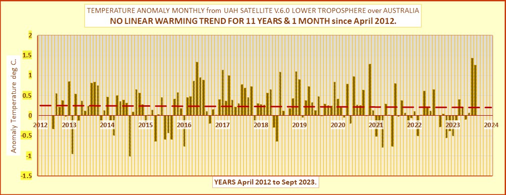
This shows the “pause” by the method of Viscount Monckton.
The high value in the last month, August b2023, has shortened the pause by knocking off the first three months.
As to the reasons for high or low valkues, or for forecasts of the future, I do not make them because I do not have a crystal ball.
Geoff S
And as I said in the previous thread, if you started that graph a couple of years earlier, in the middle of 2010, you could be seeing a warming trend of 0.37°C / decade.
But that is not what the calculation is about.
2010 was before the major 2015/2016 El Nino.
You know… those El Ninos you have to use to show any warming trend.
Therefore, nothing to do with atmospheric CO2.
El Ninos clearly do not cause a warming trend. Since they occur roughly every 3 years and it has been about 12000 years since the last ice age that means that there should have been about 4000 El Nino events since then. Now the average temperature during the last ice was about 6 degrees cooler than currently (https://www.smithsonianmag.com/smart-news/ice-age-temperature-science-how-cold-180975674/) so on average each El Nino could only have raised the temperature by 0.0015 degrees. The current rate of warming is 100 times that.
“El Ninos clearly do not cause a warming trend.”
LOL… Yet every time there is a strong El Nino we get the ONLY warming in the UAH data.
The whole “climate scare” farce RELIES TOTALLY on those El Ninos… like the last 2 months.
The whole climate complex has been PRAYING for this one. !
“LOL… Yet every time there is a strong El Nino we get the ONLY warming in the UAH data.”
Are you really that unaware of what you are writing? Does it not worry you that despite the fact that you are clearly an amateur, like (almost) all of us here, no one seems to support your “El Nino is the cause of the warming” mantra? And the monumental roadblock in front of you is…. if it was the cause, why has it not been the cause in the past? I mean El Nino’s have been around for ever, so why are we not boiling?
Simon,
Specifically, do you class me as an amateur?
Good luck with that. Geoff S
If you agree with bnice2000 that El Nino is the cause of the warming… no…. In that case I’d call you a rank amateur.
So, absolutely no counter to the facts as shown in UAH data,
Quite pathetic really.
Do you DENY that the only warming steps in the UAH data came at El Nino events !! really !!
Is your tiny mind so closed that you cannot see that fact. !
And no Simpleton, I am not an immature like you.
You obviously have a total lack of any education in the relevant fields of science, physics, maths or anything even remotely related to understanding climate.
“nd no Simpleton, I am not an immature like you.
You obviously have a total lack of any education in the relevant fields of science, physics, maths or anything even remotely related to understanding climate.”
I know that ENSO has played no direct hand in the recent warming (last 100 years) we have experienced, which is one more thing than you. So if I am a Simpleton, what does that make you?
“Is your tiny mind so closed that you cannot see that fact. !”
childish putdown. Well that is a surprise.
Uh well look at the graph sir. 1998 ——> 18 year pause. 2016———-> 6 year cooling
To be fair to Izaak’s core assertion that El Nino’s do not cause warming, it is entirely possible that El Nino’s merely release built up warmth to the atmosphere, and that without some other forcing the temperature history would show spikes at El Nino’s with a subsequent return to baseline. Whether the forcing was increased CO2 or any of numerous natural causes that haven’t been accounted for (solar insolation changes at various frequencies, strength of magnetic field, underwater volcanism, etc) could still show the same result in the temperature data.
Yeah, they keep ignoring those sudden step up warming in the data…….
The current atmospheric warming has come ONLY at El Ninos events.
So whatever the “rate” is, is what those El Ninos have provided.
Child-like calculations like your are meaningless.
There is no evidence that CO2 has caused any of the highly beneficial warming since the LIA.
Izaak,
Your comment that el ninos do not cause warming trends is unsupportable, You might as well claim that heatwaves do not cause warming trends (which at some stations is true). You are assumiong that each el nino every few years has a positive anomaly that can be summed over time. Some el ninos are relatively cool and should be subtracted, not added, depending on how you structure your analysis.
Geoff S
Hate to tell you but we are still in the same “ice age”. It has been ~12,000 years since the last massive glaciation in this ice age. We are now in an interglacial period which will end I have no doubt.
Correction, we have been in an Ice age for around the last 2.6 MILLION years, it is Glaciation and Interglacial phases that are the proper terminology.
Javier Vinos a while back showed that El-Nino’s were few and weak for long periods of time in the early interglacial time thus your numbers are waaaay off.
You made several easy to spot errors……
“But that is not what the calculation is about.’
Of course not. The calculation is about trying to give a misleading impression that warming has stopped.
“2010 was before the major 2015/2016 El Nino.”
Not sure how to break this to you, but so was 2012.
“You know… those El Ninos you have to use to show any warming trend.”
You realise that you are using those El Niños to claim no warming? The pauses always start before them, which has the effect of pushing the trend down.
But over the long term, El Niños and La Niñas have no effect. They cancel out and any trend you see is coming from else where. The trend since 1978 is 0.17°C / decade. It would be nonsense to say that that was the result of El Niños.
“Therefore, nothing to do with atmospheric CO2.”
You need to take a course in basic logic.
Since the 20’s and 30’s were the warmest part of the 20th century we are *till* in a downtrend from then. When the Dust Bowl conditions return for a decade then we can talk about if there is an up-trend or not.
“Since the 20’s and 30’s were the warmest part of the 20th century”
And your evidence for this is…? Considering you think here is no such thing as a global average temperature, and you think all global averages have uncertainties of a degree or more, I’d love to seen how you can make such a definitive statement.
“When the Dust Bowl conditions return for a decade then we can talk about if there is an up-trend or not.”
What? Surely you are not suggesting there may be negative consequences for a warmer planet.
“But over the long term, El Niños and La Niñas have no effect. “
Exactly…..
Besides co2, I wonder what might have caused the fall in temperatures between 2016 and now? 🙂
Mike,
We pay a fortune each day to the IPCC rto answer questions like that.
I do not have their computers and their measurement devices, so I would be only able to give uninformed opinion.
So I don’t.
However, I am finding Riochard Willoughby’s studies of global climate scale water movement quite interesting.
Geoff S
I think Richard might be on to something and I’m quite interested, too.
Geoff, one of the issues with the IPCC is that you do have the same computers and measuring devices as they do. You also have the required qualifications. The IPCC is merely a group consisting of one person sent from each participating government to edit the statements of scientists to meet their government’s desires. They may have more access to paywalled papers, but those are used as tools to support a conclusion rather than sources to develop an opinion.
Geoff, Do you have the Australian data as a graph for the whole satellite era?
Mike,

Sure.
I have added the linear least squares fit line and equation.
Cheers Geoff S
For those that may not know the 0.0014x term means the trend is +0.17 C/decade.
Thx. I found the trend on my own and if I recall (I threw away my work) it was quite durable. But I am one who doesn’t “know”, so where do I go to “know”?
Belay that. Months to years to decades, right?
Yeah, just multiple by 120.
Thanks Geoff.
I have next added some non-linear trends.
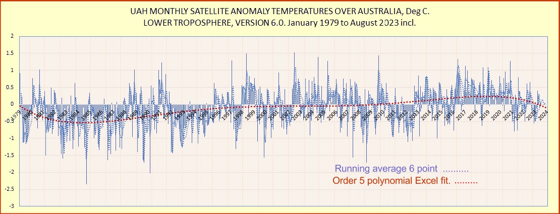
They can create impressions that follow preconceptions, but they lack mechanisms to explain them helpfully.
Geoff S
I find it challenging to find the co2 signal there.
“to find the CO2 signal there.”
There is NONE.
There is no possibility of any, because CO2 does not cause warming in the atmosphere.
If this forecast is correct (for Sept 8 + a few days after), September could see a significant drop.
After 2 months of magnificent weather, the forecast is for extended cold over a couple of weeks with strong late season snow falls in the snowfield areas of NSW and Vic.
image-20.png (768×265) (wp.com)
Cold Front Sweeping Across South-East Australia, Bringing Spring Snow to Resorts – SnowBrains
Correct in that I calculate with a 50/50 split that Australia’s UAH anomalies averaged 0.164C in January 2012 to October 2017 and 0.205C in November 2017 to August 2023 – an averaged increase of 0.041C.
Nevertheless, among surface stations within ACORN 2.3 the anomalies averaged 0.927C in January 2012 to October 2017 and 0.923C in November 2017 to August 2013 – an averaged cooling of 0.04C.
November 2017 to August 2023 includes 2019, Australia’s driest and hottest year on record.
Good point, Chris.
Geoff S
I’m not versed enough in what it all means but a couple things that stand out to me from that chart is the significant anomaly in the tropics as it has very little variability up until May of this year. The other is the significantly warming seen over Australia (east coast) for July and August which again to my understanding is being attributed to warm ocean waters off the coasts. This is from an article in the Guardian:
“One of the main contributing elements to Australia’s winter warmth was the warm ocean conditions, Hines said.Much higher than usual average surface ocean temperatures were being recorded around the world and were contributing to current local conditions, with particularly warm water off the Queensland coast.”
As specialists predicted after the Tongan eruption and switch to less opaque shipping fuels, increased SSTs have indeed boosted tropospheric temperatures. It has nothing to do with CO2, which has increased steadily since the end of WWII. For 32 years thereafter, the world cooled. Then it warmed slightly until the blow off of 1997-98 Super El Nino, then went sideways until the 2015-16 Super El Nino, followed by global cooling until the 2022 Tongan eruption.
CO2 meanwhile grew steadily, so need not apply for the man-made climate change seal of ignominy. However more plant food in the air has greatly greened the planet.
Milo,
Judith Curry has a long and interesting article about possible causes of recent heat, including the Tongan euption.
Lots of DATA, 250 or more comments.
Geoff S
https://judithcurry.com/2023/08/14/state-of-the-climate-summer-2023/
OLR has been increasing BDGWX.
Was this meant for me or Geoff?
Milo:
I gave you an Up vote, but I have a few comments
You, and so many others, claim that the 1997-1998 and 2015-16 El Ninos were natural events.
They were NOT, both were man-made, due to large reductions in the amount of SO2 aerosol pollution emitted into the troposphere (7.7 million tons, and 23 million tons, respectively) due to “Clean Air” efforts
However, the 2023 El Nino (confirmed on June 6), is being caused by the rare Hunga Tonga water volcano moisture fallout, which is flushing industrial SO2 aerosol pollution out of the troposphere, and causing temperatures to rise, making it a largely natural event.
However, there does appear to also be a man-made component, due to Net-Zero and other activities, such as the low sulfur mandate for shipping fuels, which may prolong it.
(And SST are being boosted by increased tropospheric temps, not the other way around).
So even with the anomalously hot summer in the N. Hemisphere, the trend is +1.4⁰ C over the next century. This is assuming that the trend holds. They keep saying that we need to keep it below +1.5 C. I’m pretty sure we’ll be okay, the only existential threat is our own stupidity.
The trend won’t hold. It’s a natural cycle.
The Modern Warming Period, like all such secular trends before it, consists of pro-trend and counter-trend cycles. The first pro-secular trend was roughly 1850-87, followed by a countertrend cooling cycle, c. 1887-1918, then a warming cycle 1918-45, then pronounced cooling 1945-77 (despite rising CO2), then sideways but slight warming 1978-2012, then present countertrend cooling cycle. This summer’s warming is not part of the natural cycle, but due to sporadic both natural and human causes.
Throughout the Holocene and prior epochs, the same natural cycles work under both warming and cooling secular trends.
Unless I’m even more confused, that 1.5c increase is since the start of the industrial revolution, or some place back there, not from now. 1.5C, by their calculations, has mostly already happened.
I’m not completely sure what they’re using as the starting point. If they’re basing it off of the preindustrial (LIA!) temperature, and the 1.5 degree increase has already mostly happened, then they know that the goals set by the IPCC and the Paris accord are impossible to realize, and that in the present climate, agriculture and the general environment are just fine from a climatological perspective. We obviously have other issues to deal with like wars, deforestation and so on (bird and marine life killing windmill exceptions, of course).
Yes
You are already demised.
A veritable Norwegian Blue parrot.
The only existential threat humanity faces near term is climate change policy.
After that, there is only one real threat, the next glaciation.
Only one can affect my kids
The Monckton Pause now starts in 2015/02 and has shortened to 103 months. The good news for the pause trackers is that 2023/08 will likely be included in a new pause at a higher level so there’s no reason Monckton need to stop posting about pauses.
When one pause ends, another begins, it is the beautiful circle of denial and it turns ever onward.
What denial is that……, the Monckton pause is a true statistical set up which is why people like you get so upset about it.
Right now, the pause length has been getting smaller lately if it goes long enough the pause will vanish completely surely that will make you happy………
The Monckton Pause crowd believes that the pause signals a slowing down or ending of global warming. Since those things aren’t true, and since thoughtful people have carefully pointed out why those things aren’t true, and why they haven’t been true during any previous “pause,” the Monckton Pause crowd can rightly be said to be in denial. And they will continue to be in denial as the current El Niño brings them a brand new peak from which a new pause can be formed. They’ll have plenty to keep them busy until the next El Niño year.
Everything you mention says CO2 is not the DRIVER of temperature!
El Nino – not CO2 caused,
pause – not CO2 caused.
You keep pointing out things that show CO2 is not a cause of warming. Talk about a CO2 denier!
Nobody ever said that CO2 drives El Niño or internal variability, what CO2 is said to be driving is the ongoing long term warming trend.
AlanJ the pauses are meant to put an emphasis on the NATURE of the warming. Without ESNO and volcanoes, the trend per decade is 0.09C, which is pretty benign. You also get lengthy periods in the record where there are no significant trends one way or the other. In this case, an 18 year flat or even slight cooling trend into the mid 2010s. A huge El Niño followed by a 6 year cooling trend. All of these factors call into question whether the warming is predominately natural or human caused.
These things don’t call it into question at all unless you are someone who mistakenly believes anthropogenic global warming precludes internal variability in the climate system. Global temperature is a combination of long term signal plus short term, random or quasi-cyclic variability. When you play around in the short term variance as Monckton does, you’ll quickly lose the forest for the trees.
Dismissing an 18 year pause that had plenty of internal variability as internal variability seems to be a bit of stretch.
Exactly! And, when you consider the uncertainty surrounding the data, you can get almost any trend you want.
Walter, pauses are expected. This is what happens when you superimpose oscillations (ENSO, volcanoes, solar) onto a persistent trend (CO2). In fact, if pauses were not observed it would indicate a problem with mainstream models that include the CO2 effect.
Here’s the rate of warming in UAH since 1979.
That only goes back to 1990. Here is a similar graph going back to 1979 which includes the uncertainty envelope.
Non-physical nosense.
Rate of change of rate of change?
That’s why I didn’t include the data before 1990 because it’s a bunch of not helpful nonsense. But the point I’m making is the rate of warming has been decelerating over the 21st century.
I don’t know that you can use that kind of analysis to conclude that the rate of warming is decelerating. I will say that the trend from 1979/01 to 2000/12 is +0.14 C/decade and from 2001/01 to 2023/08 it is 0.15 C/decade. Maybe the rate of warming has accelerated during the 21st century?
Is that not cherry picking?
It could be. Just understand that I’m not the one who picked it. I’m just reporting the results.
“This is what happens when you superimpose oscillations (ENSO, volcanoes, solar) onto a persistent trend (CO2). “
More “correlation is causation” from a statistician.
Have you looked into the model he is using? He’s arguing that without CO2 there wouldn’t’ be a warming trend. Again, oversimplification of the problem.
To be precise I’m arguing that the existence of pauses are not sufficient to falsify a hypothesis that CO2 is a modulating factor.
“””This is what happens when you superimpose oscillations (ENSO, volcanoes, solar) onto a persistent trend (CO2).”””
But if natural variation can be large enough to offset CO2’s temperature increase, then you can not simply do a regression based upon the max and min temps to find the temperature increase attributed to CO2. Your regression is then for natural+CO2, not just for CO2. You must first find the attribution percents first.
Let’s just say that 50% is natural and 50% is CO2. So if the anomaly is 0.7, then 0.35 is due to natural variation and 0.35 is due to CO2 growth.
What does that do to the temperature increase trend of CO2?
you didn’t really expect an answer, did you?
So CO2 doesn’t drive short-term trends but it does drive long-term trends?
Hmmm…. What is a long-term trend but a collection of short-term trends?
No one is saying that the pause indicates anything about the temperature other than CO2 is apparently not the driver or increasing CO2 would cause increasing temperature.
The only one that seems to be in denial is you. If your car stops running all of a sudden what is the cause if your gas tank (CO2) is full?
Yourself and others in this thread would say that my car stopping with a full tank of gas means that gas doesn’t make cars go. I would say that there are things other than an empty gas tank that can make a car stop running, so the car stopping for a bit does not disprove the combustion theory of locomotion.
That’s a poor analogy my friend. The climate isn’t nearly as simple as your car running out of gas. It’s a chaotic, nonlinear system. Over the past 1,000 years, the climate has had warmed and cooled in a cyclical fashion but with short term trends upon short term trends upon short term trends in between.
My comment above was pretty stupid. Over the past 1,000 years, the climate has had warmed and cooled in a cyclical fashion but with short term trends upon short term trends upon short term trends in between. That’s exactly what’s being observed now.
Does NO ONE defending CAGW have any real world mechanical experience at all? CO2 is like the gas in your car. CO2 is the fuel that makes life possible on earth and gas is the fuel that allows your car to move. But the gas doesn’t control how much power your car makes, it is a myriad of other things that does that, the fuel pump, the carburetor that mixes the gas with air which then feeds the engine, the ignition system, etc. The frequent pauses in temp rise means it isn’t CO2 that is causing the temp to go up, it is something else. CO2 didn’t make the temp go up when the interglacial period saw its first warming and it isn’t doing it now.
That is not what that means. You’re making a rudimentary error in logic. CO2 is driving a slow, steady march of temperature change, over which there are superimposed other modes of variability. Sometimes that variability is additive (el nino), other times it is subtractive (la nina, volcanoes), but the existence of those other modes of variability does not preclude the nature of CO2 as a forcing agent. Even when there is a forced response counterbalancing CO2 forcing (e.g. aerosol pollution) it still does not mean that CO2 is not a forcing agent.
A river is flowing steadily downstream under the influence of gravity. If a boulder falls into the river it will temporarily disrupt the water’s flow – even sending splashes of water back upstream. That does not mean that gravity is not driving the flow of water.
Your theory pretty much refutes the IPCC since their projections are based upon CO2 concentration driving temperature increases.
How does one know this? Because the models would not show increasing temperature if CO2 concentration quit increasing. Under that scenario NetZero would no longer be necessary.
… which is perfectly consistent with what I described above.
See what I told bdgwx. If that is the case then you can not regress the absolute values of max and min. You must do an attribution for each component and regress them separately.
You might want to investigate multivariate time series.
Did you intend to reply to me, here? Your comment is not germane to the present discussion.
“CO2 is driving a slow, steady march of temperature change, over which there are superimposed other modes of variability.”
Prove it! No one else has been able to do so. Can you?
All you have is a “correlation equals causation” argumentative fallacy.
“Sometimes that variability is additive (el nino), other times it is subtractive (la nina, volcanoes), but the existence of those other modes of variability does not preclude the nature of CO2 as a forcing agent.”
It doesn’t prove the nature of CO2 as a forcing agent. You keep using circular logic: CO2 causes warming because CO2 causes warming.
“That does not mean that gravity is not driving the flow of water.” This is backed up by proven theory and observations. Where is the proven theory for CO2?
You misunderstand me. I am not here trying to forward an argument proving that CO2 drives temperature change, I am pointing out why your argument fails to prove that it does not.
I don’t care whether you agree that CO2 drives temperature change, I’m only saying that you cannot logically use natural short term variability as evidence against CO2 as a climate forcing.
What you are saying is that if CO2 were driving temperature change, we could only observe temperatures increasing monotonically, without any variance or deviation. I am saying that is a non-sequiter. CO2 can drive warming and there can be other things influencing the temperature also. They aren’t mutually exclusive.
AlanJ,
There was plenty of ENSO and other internal variability within the hiatus period. If natural forces were able to temporarily keep the Earth’s temperature on hold for 18 years why couldn’t it have warmed the world in the prior 19 years? You can’t have it both ways. 🙁
It’s called cognitive dissonance. He thinks he *can* have it both ways!
Of course it could have, and no one is saying otherwise. ENSO is quasi-cyclic, so roughly half the time it is enhancing surface temperatures and the other half it is dampening them. This is what produces Monckton’s pauses.
When you argue that pauses and natural variability are expected, that makes it hard to know what the difference is between a naturally forced warming trend is and a CO2 forced warming trend. Supposedly prior to 1900, all of the change that occurred in the Earth’s climate was natural.
Of course it is difficult, that’s why tons of really smart people have spent so much time and effort trying to figure it all out.
“ I am not here trying to forward an argument proving that CO2 drives temperature change”
Of course you are!
“I am pointing out why your argument fails to prove that it does not.”
Your circular logic chain can’t prove anything.
I, on the other hand, can point to the 1920’s and 30’s to show its been just as hot *before* today’s level of CO2 growth in the atmosphere. *Something* cause the 30’s temps to go up. Why isn’t the reason for that a subject of intense scrutiny? That reason would be the most likely culprit for temp rise today, not CO2.
Tim Gorman:
The rise in temperatures during the depression of the early 1930’s was because of the decrease in industrial activity, resulting in less SO2 pollution of the atmosphere, and therefore much higher temperatures.
Between 1929 and 1932 there was a 13 million ton decrease in those emissions. By way of comparison, a VEI4 eruption typically puts 0.2 million tons of SO2 into the stratosphere, and causes, on average, 0.2 deg. C. of warming when they settle out
The later warming during the Dust Bowl of 1935-38 was due to a heat dome, or stalled high pressure weather system The SO2 aerosols in the air trapped within those systems, quickly settles out, again, causing temperatures to rise.
And you are correct, the current El Nino is also caused by decreased SO2 aerosols in the atmosphere, due to their being flushed out by the moisture from the Hunga Tonga eruption.
You don’t even have to agree with what you assert to understand that it represents alternative theories for the “global temperature”. As such they need to be included in any modeling, they can’t just be ignored. If they give similar results to CO2 then how do you differentiate between the models?
Tim Gorman:
All El Ninos are random events, and therefore can never be modeled.
The control knob for Earth’s climate is the simply the amount of SO2 aerosols circulating in its atmosphere
Increased them, and it cools down. Decrease them and it warms up.
This is a non-response and looks like an attempt to pivot the conversation. I’ve not employed circular logic. You’re saying, “if CO2 were a warming agent there could be no climate variability.” I’m saying your conclusion does not follow from your premise. You can have both things. If you want to forward this as an argument against CO2 as a warming agent you need to demonstrate that climate variability is incompatible with CO2 acting as a warming agent.
This is elementary logic. If A then not B. B therefore not A. That only works if you can establish the premise A then not B, and you haven’t even come close to doing that.
That is his modus operandi. He tried it with me below. Like you I’m only arguing that if model M predicts pause P and P is observed then you cannot say that M is false. In formal logic the argument is M → P. However, he twists that conditional and claims I’m arguing P → M instead which is not only something I never advocated for but its also absurd.
And BTW…it almost defies credulity to think that there are at least 2 people here that think that an observation of a prediction necessarily means that the model that made that prediction is wrong. Seriously?
bdgwx – In formal logic the argument is M → P.
The formal logic of a conditional statement uses “p” and “q”.
With your assertion:
p => I expect pauses
q => pauses do not refute CO2 warming.
A conditional statement is:
If p, then q
the contrapositive statement is:
If ~q, then ~p
The contrapositive must be true for the conditional to be true.
So you end up as I told you.
Conditional – If I expect pauses, then pauses do not refute CO2 warming.
Contrapositive – If pauses do refute CO2 warming, then I do not expect pauses.
The contrapositive is false because you do expect pauses. Therefore, the conditional must be false also. Yet you say it is true.
In other words circular reasoning that can’t be refuted.
Maybe you could come up with a real falsifiable assertion that is pertinent. Try using facts rather than what you simply believe.
It is not my assertion. It is yours. And as I have told you repeatedly don’t expect me to defend your assertions especially when they are absurd.
No I do not. You made up a stupid conditional. It’s yours and yours alone. And as I have told you repeatedly don’t expect me to defend your arguments especially when they are absurd.
I will repeat again hopefully this time in clear and concise language that cannot be misconstrued, misrepresented, or twisted…the model M makes prediction P. If M is true then P is true. Observing that prediction P did, in fact, occur is not sufficient to falsify M. Do you understand this concept. Yes or No? Don’t deflect. Don’t divert. Don’t make up absurd statements/arguments I never said or advocated for. Just answer the question and provide commentary related it and only it. I don’t care if you use conditional/contrapositive logic. Just form the conditional based on what I said and not something absurd that you and you alone made up.
p = pauses exist
q = pauses are not sufficient to falsify CO2 modulates
~p = pauses do not exist
~q = pauses are sufficient to falsify CO2 modulates
Conditional
If pauses exist, then pauses are not sufficient to falsify CO2 modulates.
Result => True by definition
Contrapositive
If pauses are sufficient to falsify CO2 modulates, then pauses do not exist.
Result => False – pauses do exist
Create your own phrases that mean the same, it won’t change the result. For a Conditional statement to be true, its Contrapositive statement must also be true.
Think about the greenhouse theory.
p = CO2 absorbs radiation
q = temperatures do rise
~p = CO2 does not absorb radiation
~q = temperatures do not rise
Conditional
If CO2 absorbs radiation, then temperatures do rise. -True
Contrapositive
If temperatures do not rise, then CO2 does not absorb radiation. – True
That is how you form a hypothesis without factual data to prove the hypothesis. It must be logical at the start. Is it falsifiable? That is the question only evidence can prove. However, it will withstand a logical analysis.
That’s not my P. That’s not my Q. At this point you’ve left me no choice but to accept that you are either unwilling or unable to discuss what I’m saying.
So your P is *not* “pauses exist?
ROFL! Is that the best you can do?
Define your “p” and “q” and it can be evaluated.
I don’t believe I have misconstrued your assertion. If you have another way to assign an antecedent (p) and a consequent (q) that fits your assertion, then do so.
You’ve forgotten the concept of conjunctions/disjunctions in formal logic. See if you can work them into your example above. I am trying with every ounce of grace I possess to view your efforts here in a charitable way but you are making it difficult.
“If M is true then P is true. Observing that prediction P did, in fact, occur is not sufficient to falsify M. “
P being true doesn’t make M a true predictor. Even a stopped clock predicts the correct time twice a day.
Strawman. I didn’t say that it did. That is your argument. You own it. I’ll repeat again…don’t expect me to defend your arguments especially when they are absurd.
This notion that CO2 driven warming could only produce a monotonic warming trend with no variance whatsoever is one of the most peculiar lines of nonsense the skeptic crowd likes to insist on. It’s such a deep misunderstanding of a simple logical concept that it is difficult to articulate a counterpoint that is uncomplicated enough that someone who failed to understand in the first place could grasp. A real exercise in “ELI5” capability.
The issue is not if CO2 could produce a monotonic warming with no variance. However, this is what the greenhouse and radiative theories do predict.
The real problem is what the warming trend of CO2 really is. By using the complete ΔT trends as evidence of CO2 warming, the IMPLICIT assumption IS that CO2 DOES cause the entire warming.
What you are attempting to say is that there is a modulating signal from other sources applied to the CO2 signal.
You must remove that modulating signal before you can observe the CO2 signal. One way to remove it is to assign percentages to the two signals
What is the result? The CO2 warming will be reduced. The rate of growth shown by the CO2 trendline will be something less per decade than what is being claimed. IOW, a deathknell for CAGW.
Incorrect. The theory says if you hypothetically had a monotonic increase in CO2 with no other forcing agents acting on the climate system or any modes of internal (unforced) variability, then you would expect a monotonic increase in temperature. The theory says that if you do have other forcing agents and modes of natural variability acting on the system, then you expect to see a signal modulated by other forcing mechanisms and overlaid by unforced variance. All climate models, both computer models and theoretical physical models, consider the full system with multiple forcing agents and modes of internal variability. For instance, this is a visual showing the net historical forcings included in CMIP6 experiments:
It is not just CO2, you have aerosol forcing, natural forcing from the sun and volcanoes, etc. And that is not including unforced variability, which models also simulate.
What you are trying to argue is that observations defy theory – you’re saying the theory demands a static system with no other forcing agents apart CO2 forcing, and that isn’t remotely true. The theory incorporates numerous drivers of temperature, natural and anthropogenic. The theory tells us we should see variance superimposed on the long term trend, it even tells us we should see the long term trend modulated by natural forcing agents like the sun and volcanoes.
The amount of warming attributed to CO2 already accounts for the fact that there are multiple influences on the climate. Scientists are not using simple linear regression of historical data to determine sensitivity, they are using mathematical models that rely on the laws of physics.
So why the need to “hindcast” and “tune” these beasts?
Because model development is an ongoing endeavor. Perfect models require perfect understanding of the climate, which is not a promise science makes.
Nice waffles. Got any maple syrup?
You are making up staw men. The idea is simple as you say.
You said.
“””The theory says if you hypothetically had a monotonic increase in CO2 with no other forcing agents acting on the climate system or any modes of internal (unforced) variability, then you would expect a monotonic increase in temperature.”””
See that last phrase.
“… then you would expect a monotonic increase in temperature.”””
That is what the greenhouse and radiative theories are based upon.
The remainder of your post deals with natural variation. If natural variation is what causes a pause in the rise of temperature, then natural variation and CO2 increase must offset, i.e., a 50/50% of the temperature change.
My point is that if you want to isolate CO2 temperature rise, you must subtract the natural variation part of any temperature change.
You cannot say that a change of 0.69 is all due to CO2! You must attribute a percent to each component. If the percents are 50/50% then all ΔT’s must be reduced by 50% if you want to see the CO2 contribution.
Address the last paragraph instead of throwing up strawmen.
No, I’m restating for the umpteenth time the singular argument I’ve made in this entire discussion, which you have been ignoring. The greenhouse and radiative theories of heat transfer do not preclude modes of natural variability in the climate system. Observing modes of natural variability does not contradict these theories.
No one is saying this. You can see in the graph I provided above that numerous forcing agents are being considered, that forcing is what produces temperature change. Natural variability on short timescales is quite large, versus GHG forcing which is small on interannual or sub-decadal timescales. The amplitude of natural variability does not mean that GHG forcing over longer timescales is not significant.
But your trend line is based upon “ΔT(CO2)+ΔT(NATURAL)”
CO2 temperature growth (ΔT(CO2)) must be less than the total. It is ΔT(CO2) only.
And remember, if you use less than 50% natural variation, then you can’t possibly have a pause.
Fair enough.
ΔT(NATURAL) might also be negative. Note in the graph above the net long term natural forcing component is slightly negative.
Unforced internal variation can be well over 50% on short time scales. That’s the whole reason we don’t try to identify long term (forced) trends using a few years of data, like Monckton does. You don’t get “pauses” when you look at time frames outside the range of typical internal variance. The forced component dominates.
Meaning CO2 must be less than 50% on short time scales. If it’s less than 50% on short time scales then what changes to make it more than 50% over long time scales? The physics don’t change for CO2.
What changes to make it over 50% on long timescales is that the unforced variation signal is bipolar – it oscillates between positive and negative and the net contribution to any long term trend is zero. Extra warmth during El Niño is counterbalanced by extra coolness during La Niña, for instance. Unforced variability by its nature is not directional (otherwise it would be forced variation – driving the system to a new energy state).
Imagine a ball rolling down a hill at 1 meter per second. After one minute it will have moved 6 meters. Suppose that every 15 seconds, someone kicks the ball up the hill 100 meters. After a minute, the ball would have moved 6 – 100 – 100 – 100 – 100 meters, or 394 meters up the hill. That’s a lot of reverse movement uphill. Now imagine that someone else kicks the ball 100 meters down the hill at alternating 15 second intervals. How far will the ball have moved in a minute? In ten minutes? in a day?
If you can understand this concept you can understand why the slow, steady march of forced climate change can dominate over unforced internal variability over the long term. Unforced variability doesn’t add energy to the system, it can’t drive a change in state.
Jim Gorman:
Yesterday you had suggested that the cause of the 1930’s temps should be investigated, since that would most likely be the culprit for the temp rise of today.
You are correct!
I provided the answer in a post shortly above, but apparently you have not read it, as yet..
You didn’t address the issue. If CO2 is causing the warming trend then the other factors aren’t a factor.
If other factors *do* in fact exist then the warming trend is *NOT* totally due to CO2 and the increase in global warming can’t be attributed totally to CO2, especially anthropogenic CO2.
So why the focus only on CO2 as if it is the only culprit?
AlanJ:
AlanJ.
Tim Gorman is correct.
“If CO2 were a warming agent, there could be no climate variability”
The slopes of CO2 increases and average anomalous global temperatures have diverged since 1980, demonstrating a lack of correlation.
“...increasing CO2 would cause increasing temperature.”
Unless, due to some fantastic coincidence your pause started just before a massive El Niño.
“If your car stops running all of a sudden what is the cause if your gas tank (CO2) is full?”
Do they have breaks on cars, where you come from?
“Do they have breaks on cars, where you come from?”
You really should stay out of threads concerning mechanical things. You don’t know squat about the real world.
Breaks (brakes?) don’t make cars stop running, they make the car stop moving.
I see you ignored the first part of my commen – the one pointing out that your pause starts just before the big El Niño.
As to the pedantry about your dumb car metaphor, the point is you have the logic backwards as usual. You are saying if a car has fuel but doesn’t run, that proves you don’t need fuel to make the car run. If you can’t see how that logic doesn’t make sense I’m not sure if I can help you.
“You are saying if a car has fuel but doesn’t run, that proves you don’t need fuel to make the car run.”
Your reading comprehension is just ATROCIOUS! If the car has gas but isn’t running then IT’S NOT THE GAS THAT IS CAUSING IT TO NOT RUN!
A coherent theory of global average temperature would be OMPLETE. It would explain each factor and its percentage of attribution to temperature rise.
Yet all we get from climate science is a graph showing correlation between CO2 and temperature – nothing, NOTHING showing any causal relationship.
The Monckton Pause crowd believes that the pause signals a slowing down or ending of global warming. Since those things aren’t true, and since thoughtful people have carefully pointed out why those things aren’t true
What a load of nonsense. How can anyone know (let alone show) this pause does not signal a slowing down or end of global warming? Perhaps you are close friends with this bloke?
It is based on the positive planetary energy imbalance and the 1LOT and 2LOT.
Well whoopty doo!
It’s based on “correlation is causation”. Warming temps could just as easily be the cause of rising CO2. Or they may not be causally related at all!
https://www.drroyspencer.com/2023/08/sitys-climate-models-do-not-conserve-mass-or-energy/
Maybe you forgot to read this. I see you didn’t post on the article when it appeared here.
Bdgwx.
This is your logic.
That’s not my graph or logic. I’m not even making statements about organic food sales or autism. I’m talking pauses in UAH TLT and whether they are inconsistent with models that includes CO2 as a modulating effect.
If you want to talk modulation, then you must know the modulating power (natural variation) and the constant carrier power (CO2).
It means your carrier power will be lower than the (modulation+carrier). Your rate per time step is going to be substantially reduced.
Correlation does not equal causation. You are arguing based on your model that Earth would not be warming if not for CO2.
Not exactly. In this discussion I’m only arguing that the existence of pauses are not sufficient to falsify the hypothesis that CO2 has a modulating effect. The reason you cannot use pauses as a falsification test is because we are expecting pauses. It’s no different than saying gravity cannot have an effect on an apples height because we observe apples falling from trees.
AGW and GHE both assume that there is a direct warming from human generated warming. Pauses are a direct refutation of that hypothesis. Without CO2 warming there is no need for NetZero.
The fact that “you expect” pauses , therefore pauses don’t refute CO2 warming is circular reasoning at its best. A perfect example of a non-falsefiable assertion.
What a great assertion to test the logic of.
Conditional.
If I expect pauses, then pauses do not refute CO2 warming.
Contrapositive
If pauses do refute CO2 warming, then I do not expect pauses.
Your assertion does not allow the contrapositive to be true.
Logic says the contrapositive must be true for the conditional to be true and vice versa.
Do you see the problem with circular reasoning? The contrapositive can not be true if the conditional is true. You just set up a non-falsefiable condition.
The real truth is that we do not know how the multivariate atmosphere interacts between all the components. Real attribution studies need to be created in order to allocate the contributions of each component.
The pause shows there is no direct relationship between the increase in CO2 and the increase in temperature. The longer the pause, the less likelihood that there is a lag between CO2 increase and temperature.
Some studies show a decrease in clouds has caused the latest warming and not CO2. These factors indicate that models which are driven by CO2 concentration will never accurately forecast future temperature.
The clown show is in full swing…
Leftists are hilariously pushing their silly CAGW catastrophism nonsense during a strong El Nino cycle, plus the warming effect of 45 million metric tons of water vapor dumped into the stratosphere following the Tonga eruption…
The PDO cool cycle has already entered its 30-year cool cycle and the AMO will likely enter its 30-year cool cycle from around 2025 which will likely lead to 30+ years of global cooling from around 2025 as experienced during the PDO/AMO cool cycles from 1880~1913 and from 1945~1980.
it’s interesting to note the current PDO/AMO warm cycle warming trend (0.14C/decade: 1980~present) is almost identical to the last 30-year PDO/AMO warm cycle trend of 0.12C/decade (1913~1945).
We’ve enjoyed about 1.2C of beneficial global warming recovery since the end of the Little Ice Age in 1850, of which, roughly 50% was from natural forcing effects and 50% from CO2 forcing… who care?… it’s a joke.
Leftist political hacks have wasted $10’s of trillions on this absurd CAGW farce and have destroyed the scientific establishment’s integrity by replacing the scientific method with Leftists’ political lust for: power, control and money.
Have I missed it or has someone come up with a plausible explanation of how a splash of water 18 months earlier finally led to a warming spike? Its only a nice excuse if you can describe the mechanism.
You have missed it, discussed in great detail in many posts and comments here. Just one post:
https://wattsupwiththat.com/2023/08/05/record-global-temperatures-driven-by-hunga-tonga-volcanic-water-vapor-visualized/
AndyHce:
I have posted a link twice on this thread, explaining the mechanism. But here it is, again
https://doi.org/10.30574/wjarr.2023.19.2.1660
The pendulum always swings back, and nature will catch up with them one day. A cooling trend would be kinda crazyyy.
Walter-san:
There has been a 100% correlation since 1850 of global temperatures rising during PDO/AMO 30-year warming cycles and global temperatures falling during PDO/AMO cool cycles…
Towards the end of the last PDO/AMO cool cycles, global temperatures fell and polar ice extents increased to such an extent, the same “scientists” who now predict catastrophic global warming, predicted we were entering a new “Ice Age”, caused by manmade coal particulates blocking the sun and catastrophically cooling the planet…
Of course when the PDO/AMO cycles switched to their respective 30-year warm cycles in 1980, and global temperatures started to rise, and the the silky manmade global cool mania was suddenly abandoned and replaced with the manmade global warming hysteria…
Leftists are so hilarious…
That’s arctic sea ice stopped falling 16 years ago. 2023’s sea ice extent is higher than 2007 last time I checked.
The Arctic sea ice area is already below the 2007 minimum and the extent is very close, may well still result in a lower minimum.
“it’s interesting to note the current PDO/AMO warm cycle warming trend (0.14C/decade: 1980~present) is almost identical to the last 30-year PDO/AMO warm cycle trend of 0.12C/decade (1913~1945).”
Yes, and in the United States, the highpoint temperatures in the 1930’s are warmer than the temperatures today. The United States has been in a temperaure downtrend since the 1930’s. No CO2 worries here.
I posted this graphic above, but I’ll do it here, too, since you are talking about past warming and cooling cycles.
Everyone needs to keep in mind that all El Ninos since at least 1850 have been TEMPORARY periods of higher temperatures, so today’s higher El Nino temperatures are to be expected, and really nothing to get excited about. Historically, they will decrease..
For the period 1900 to 2022, their durations ranged from 6 to 23 months, with an average of 10.5 months.
The warmer July and August this year are not due to a growing El Nino alone.
Milo:
Yes, I think that is correct.
July and August were nothing special with regard to temperatures this year where I live. It’s been a lot hotter in the past around here.
El Ninos are the removal of excess ocean heat stored during the previous 5 to 8 years so it can be vented to space — a cooling mechanism.
AndyHce
No, Andy, that is nonsense!
All El Ninos are due to decreased levels of SO2 aerosols in our atmosphere
https://doi.org/10.30574/wjarr.2012.17.1.0124
The 0.69 C anomaly corresponds with an ONI of -0.1 or 0.2 depending on whether the lag is 4 or 5 months. In other words we haven’t seen the El Nino response in UAH TLT yet.
You forgot to include the ZBZ in this calculation.
August was the first month since May 2017 that Aotearoa New Zealand experienced colder-than-average temperatures, and it was the coldest August since 2016. The nationwide average temperature in August 2023 was 8.4°C. This was 0.55°C below the 1991-2020 August average according to NIWA’s seven station temperature series, which began in 1909, and just scraping in as “below average” (the threshold for below average is more than 0.5°C below the 1991-2020 average).
Not that it means anything but it still looks cooler than 2016
Which is very bad. I want to see us continue to warm out of the LIA, no stinking pauses please.
I want at least medieval aa period warmth, maybe even Roman.
Pick your golden age and wish upon a star.
Got my first “posting too fast message” as I tried to correct my aa to warm.
I type with one thumb on my phone
No one ever accused me of going too fast.
Sorry Pat but, given the long term trend from the Holocene maximum into the next glacial, I just don’t think temperatures in the Modern Warming period will ever get to that sustained level. It’s downhill all the way, I’m afraid.
Richard Page:
Maximum Holocene temperatures were a disaster for mankind, lets hope we never reach that level again.
However, I do fear that we will reach it in a couple of years.
Why do we have heat waves in North America and Europe? When the solar wind weakens, the speed of the jet stream current at high latitudes also weakens. The jet stream descends in the eastern Pacific and Atlantic, forming meanders. The curves over North America and Europe form stable highs with warm air from the south. Water vapor in these highs remains gaseous and reduces the vertical temperature gradient. The surface warms up so much that the temperature drop is not strong at night.

It is the jet stream in the tropopause that creates the major highs and lows.
In the current solar cycle, the solar wind is rippling. A brief increase in speed is followed by a sharp decrease.

If this keeps up we might have to start sacrificing politicians to appease the gods.
Didn’t sacrifices involve something of value, such as goats or bulls?
Damn, well that rules out reality tv ‘stars’, insurance sales staff and students, among others.
There’s a chap in Hamelin who might be able to help with them.
The Sputnik here is recording 2 things:
1a Increasing Aridity of Earth’s land surface, causing…..
1b ……the expansion of heat domes over farmland, burnt forest and ever expanding cities ###
….and….
2a Rising sea levels
2b The sea is rising because of (1a) above
Your teacher at Kindergarten, though you loved her dearly and trusted her implicitly, lied to you about 3 things which are relevant here:
1/ Dry land is NOT supposed to be dry
2/ Carbon Dioxide does not ‘fertilise’ plants any more than water does
3/ (and a partial partial mistruth when she asserted that) ‘Hot Air rises‘
Yes it does but air that is merely = ‘warm‘ and contains water vapour rises much faster
i.e. and e.g. Hot air balloons do not fly because the air inside them is hot & dry
(They would melt and or burn)
They fly because the air they contain is warm and moist.
Thus an ‘electric hot air balloon‘ would never work – you need something/anything that fills your ballon with warm water vapour . e.g. Propane, butane, kerosene, gasoline or even, coal.
Hot air balloons are actually = Warm water-vapour balloons
And THAT little factoid is what creates ‘weather‘ and thus ‘Climate‘
### I am sincerely hoping and praying that The Sputnik *is* doing an area weighted measurement
Gosh! Tiny fractions of a degree – it must be science with such precision.
Didn’t I read somewhere that meteorological thermometers are only accurate to about +/-0.5C? And they are not calibrated to a standard reference instrument either.
Therefore global average temperatures are fictional.
[Christy et al. 2003] say the uncertainty is ±0.2 C.
NOT an uncertainty analysis: instrumental uncertainties ignored, all variances from all averages deleted and ignored.
Have you explained this to Drs Spencer and Chrisity yet? If so what was their response?
Why do you care?
And from that climate science tries to extract differences in the hundredths digit?
ROFL!!
So the uncertainty interval is 0.49 – 0.89. Do you know where in that interval the real value lies? What is the confidence of that interval.
What is the possible lowest trend? What is the highest possible trend.
They don’t know either! That uncertainty interval is like a fishbowl full of milk that has a floating gem in it somewhere. They then guess at a location somewhere in the fishbowl based on subjective biases but they have no real knowledge of whether its the right location or not. But to them it is the RIGHT SPOT! Just like the temperature is exactly what they say it is!
“Do you know where in that interval the real value lies?”
What part of the word “uncertainty” don’t you understand?
“What is the confidence of that interval.”
If it’s a 2σ range, about 95%.
“What is the possible lowest trend? What is the highest possible trend.”
Define impossible. Theoretically anything is possible, so -infinity to +infinity.
Here’s what the August UAH anomalies look like, including the assumed ±0.2°C monthly uncertainty.
There is some overlap with 1998, so conceivably if the error this year was high, and the error in 1998 negative, then it’s just possible that 1998 was warmer than 2023.
But…
First, of all how likely is this given random errors each month. I ran a simple Monte Carlo simulation, assuming a normal random error with sd = 0.1 for each month.
The result is there would be a 97% chance that 2023 was the warmest August, with 1998 only a 1.7% chance of being warmer. Other recent years have a small (< 1%) of being the warmest. Here are the probabilities for all years with a better than 1 in a 1000 chance of having the warmest August.
However, I donlt think this makes much sense for a few of reasons:
Just for fun, I wondered what the probabilities would be if the we used were karlomonte’s fantasy 0.5°C standard uncertainty.
The probability of this month being the warmest August drops to just 21%, but probability of 1998 being warmest is only 8%.
Of course, nearly every year has a chance of having the warmest August, but it’s the more recent months that generally have the best chance. The chance that the warmest August occurring in the last 10 years is over 50%.
Here are the top ten probabilities
Trendology at its nadir…
That’s talking about the earlier version – I would assume version 6 is claimed to be better. Also it seems they actually say the standard error for a month is 0.1°C, and for a year 0.07°C.
As, a quick test I compared the difference between month anomalies for UAH and GISS. The standard deviation was 0.16°C, which seems reasonable given they are measuring slightly different things.
For annual averages the SD of the differences was 0.1°C.
You do realize that analyzing the SD for anomalies by using the anomaly values is actually performing math magic, right?
At least for GISS, anomalies should carry the variance (SD) of the absolute temperatures used to calculate them. They are subtracted random variables.
Always the magic of averaging…
Bwahahahahahahahah
It’s Spencer and Christy you’re laughing at. If you don’t agree with their figure you can explain it to them.
No, it is YOU who is here quoting and pushing this milli-Kelvin nonsense, it is glaringly obvious that you believe these ridiculous numbers are valid.
Why would you think I believe anything those two claim?
So far, all your arguments amount to “wha, wha, the uncertainties can’t be that small – don’t like it.”
If you want to convince anyone that the uncertainties are much bigger, you need to provide evidence, but don’t bother me with it – tell the people who actually run the thing.
Pssssst, LoopholeMan, you’ve been told countless times—I’m done trying to educate you, you are hapless and hopeless.
All that is left is to point and laugh.
And for the record, it isn’t my job to do what S & C refuse to do.
“And for the record, it isn’t my job to do what S & C refuse to do.”
Of course not. It’s just your job to spew out unfounded allegations whilst laughing manically.
The checklist:
instrumental uncertainties — unknown, ignored
# of points averaged in a month — ignored, not reported
standard deviations of monthly averages — ignored, dropped
ditto all other averages down the line — ignored, dropped
The standard deviations that can be backed out of the data files are on the order of DEGREES, not milli-Kelvin.
Unfounded allegations indeed, LoopholeMan.
You’re telling the wrong person. If you think Spencer and Christy don;t understand what they are doing, you need to tell them, so they can improve their uncertainty estimate – or we could just never talk about UAH, pauses and reality meters ever again.
Again showing you don’t care about reality but will plow straight ahead quoting this 70 mK fantasy over and over. The subject has been broached with Spencer, and he made it quite clear that he doesn’t care either.
Christopher sure has a burr under your saddle, he saw through your act a long time ago, and you whine endlessly about “pauses”.
Here is the problem UAH has in my opinion. Look at the variation in data over the last one year and 8 months. The low is -0.04 while the high is 0.69.
The standard deviation is 0.19! That is an uncertainty in the tenths digit 0.2
So an interval statement of 0.23 ±0.2.
Now let’s divide the SD by that √20 and we get ±0.04. So the interval statement is 0.23 ±0.04.
From the GUM.
2.2.3
uncertainty (of measurement) parameter, associated with the result of a measurement, that characterizes the dispersion of the values that could reasonably be attributed to the measurand
If the measurand is the mean, as you are want to do, which interval statement better describes the dispersion of values that could reasonably be attributed to the measurand?
Remember the two intervals are:
0.23 ± 0.04 => 0.19 to 0.27
0.23 ± 0.2 => 0.03 to 0.43
And, the range is from -0.04 to 0.69.
Which better describes the dispersion around the mean?
“The standard deviation is 0.19! That is an uncertainty in the tenths digit 0.2
So an interval statement of 0.23 ±0.2”
The problem here is you are assuming all the values are random variation around a mean.
And as I’ve said before you have to know what uncertainty you want. Looking at the SEM of all months isn’t telling you how close the reported monthly value is to the actual value. It ‘s more about telling you how much variation there might have been in an annual average, if the monthly values had been different.
“Now let’s divide the SD by that √20 …”
Where did the 20 come from? If I understand you, you are trying to calculate the SEM for the year so far, but there have only been 8 months.
“From the GUM”
For the sake of my bandwidth could you just assume I know the GUM definition of uncertainty.
“Remember the two intervals are:”
Well the second one is closest to the stated measurement uncertainty, so I would say that one.
“Which better describes the dispersion around the mean”
That isn’t the definition. It’s the dispersion of values that could reasonably be attributed to the mean. Not how much dispersion there is around the mean.
“””That isn’t the definition. It’s the dispersion of values that could reasonably be attributed to the mean.”””
Guess again. I’ve attached the definition again. I do not see the word “MEAN” mentioned at all.
2.2.3
uncertainty (of measurement) parameter, associated with the result of a measurement, that characterizes the dispersion of the values that could reasonably be attributed to the measurand
Forget the mean. It is really only needed to calculate the Standard Deviation. The GUM has deprecated the term “true value” for a reason. There is no true value anymore. The mean is just the middle of an interval where the measurand may lay.
I don’t how to explain uncertainty to you any better than the GUM does.
Uncertainty is an interval that “characterizes the dispersion OF VALUES …”
The SEM does not characterize the dispersion of values. It characterizes the interval where a mean can lay. Those are two different things.
To display your understanding you need to tell why the units digit doesn’t define the uncertainty.
“I do not see the word “MEAN” mentioned at all.”
As you said, the mean is the mesaurand in this case.
“The GUM has deprecated the term “true value” for a reason”
Yes, because they say it’s a tautology, and it’s only an idealized concept –
“Forget the mean. It is really only needed to calculate the Standard Deviation.”
Except when the mean is the thing we are interested in – as in a global mean anomaly.
“Uncertainty is an interval that “characterizes the dispersion OF VALUES …””
You keep cutting and pasting, but still don’t seem to read it. “characterizes the dispersion of values that could reasonably be attributed to the measurand””
You seem to confuse this with the dispursion of values that went into creating the mean. It’s not, it’s the range of values it might be reasonable to assume the measurand (in this case the mean) can be.
“The SEM does not characterize the dispersion of values.”
But it does characterize the dispersion of values that could reasonably be attributed to the mean.
“It characterizes the interval where a mean can lay.”
where the mean could reasonably lay.
“As you said, the mean is the mesaurand in this case.”
You said earlier that the average doesn’t actually exist. So how can it be a measureand if it doesn’t actually exist?
No. The average exists. It just doesn’t have to exist as a concrete object.
If the average doesn’t represent a measurable object then it can’t be measured. It isn’t and can’t be a measurand. Thus it can have no measuremnet uncertainty. It can have a “calculation uncertainty” but that is *not* the same thing as a measurement uncertainty.
Several of us have wasted countless hours trying to educate you on this subject and yet you remain stubbornly and willfully ignorant on the subject.
In physical science you can measure the force of gravity multiple times in multiple experiments and the average of those measurements represent a physical thing – the force of gravity.
In engineering you can measure the shear strength of a beam multiple times and the average represents a physical thing – the shear strength of a beam.
In mechanics you can measure the diameter of a crankshaft journal multiple times and the average represents a physical thing – the diameter of that crankshaft journal.
In none of these can you increase the resolution of the average value through averaging. The resolution of the average remains determined solely by the resolution of the measuring device. It is the height of folly to suggest that your measurement resolution is anything else.
In physical science you can measure the force of gravity on several different planets and combine them into a data set. Their average value, however, exists no where. It can’t be measured. Therefore the average value can’t be a measurand. The average remains nothing but a calculation result You can calculate how closely you can calculate the population average from a sample of the data but it remains nothing but a calculation result, it is not and cannot be a measurement uncertainty of a measurand.
In engineering you can measure the shear strength of a collection of different things, e.g. 4″ i-beams, 1/4″ steel rods, a wrought iron railing; combine them into a data set and calculate their average value. That average value, however, exists no where. It can’t be measured. Therefore the average value can’t be a meassurand. The average remains nothing but a calculation result. You can calculate how closely you can calculte the population average from a sample of the data but it remains nothing but a calculation result. It is not and cannot be a measurement uncertainty of a measurand.
You can play with numbers all you want but unless they represent a physical result all you are doing is mental masturbation. If you can’t recognize that 1.x1 +/- u1, 2.x2 +/- u2, 3.x3 +/- u3, 4.x4 +/- u4, etc represents a multi-modal distribution then you are truly lost in the forest of the number line. The average of those numbers represent nothing physical and therefore can’t be a measurand. It simply doesn’t matter how many decimal digits you carry out the calculation of the average or what the standard deviation of the sample means turns out to be – you won’t be calculating measurement uncertainty. The measurement uncertainty remains a function of the units digit and the range of those measurements is such that the uncertainty is so high that the average is unusable for anything physical.
If you can’t, or won’t, understand the point of this very long post that took me a lot of time to author then you are nothing but a troll posting click-bait. I’m done with you.
And as Jim always says, it can’t be blindly plugged into GUM eq. 10.
You didn’t answer my question.
To display your understanding you need to tell why the units digit doesn’t define the uncertainty.
I should specify that I am talking about the 5 numbers you listed that ranged from 10+ to 13+ with 5 decimal places.
If you can’t answer this question, then your understanding is faulty.
“You didn’t answer my question.”
km_mode: You are in no position to make demands on me, I’m not going to succumb to your Jedi Mind Tricks, you wouldn’t understand the answer, I’m done trying to edumacate you.
OK, now I’ve got that out of my system.
“To display your understanding you need to tell why the units digit doesn’t define the uncertainty.”
“I should specify that I am talking about the 5 numbers you listed that ranged from 10+ to 13+ with 5 decimal places.”
Why would the units define the uncertainty. The rods range from 10 to 14, and are taking from a uniform distribution, so the standard uncertainty is 2 / √3 ≈ 1.15, if that’s what you mean. the range defines the uncertainty in this case.
But the uncertainty of the mean (i,e, SEM) is σ / √5 ≈ 0.52.
“If you can’t answer this question, then your understanding is faulty.”
You say that is if you think you understand something. So far I’ve seen little evidence of that.
^^^^ Owned.
“””Why would the units define the uncertainty. The rods range from 10 to 14, and are taking from a uniform distribution, so the standard uncertainty is 2 / √3 ≈ 1.15, if that’s what you mean. the range defines the uncertainty in this case.”””
10.07374, 12.26802, 13.44460, 11.92005, 12.95371
From a online standard deviation calculator.
Count, N: 5
Sum, Σx: 60.66012
Mean, x̄: 12.132024
Variance, s2: 1.67449613793
s = √1.67449613793
= 1.2940232370132
The standard uncertainty is 1.3.
Do you not understand what that is telling you? The uncertainty is in the units digit, i.e., the digit “1”.
If you were building a road, is the distance 10 mi. vs 13 not a big distance?
Is an artillery target variable from 10 to 13 km? Could 10 km be on top of your troops and 13 km on the enemy?
Is you driving such that you need 13 meters to stop ok when there is a wall at 10 meters?
How about ordering 10 yards of concrete when you need 13 yards?
Is 10° vs 13° a big difference when measuring parallax of an interstellar object.
Measurements matter. Total uncertainty matters. Averages not so much.
I forgot to add. Per TN 1900, the expanded experimental standard uncertainty.
1.2940232370132 / √5 = 0.57870478447985452789 • 2.776 = 1.6.
Still in the units digit.
Now do it for the 1000 rod example.
Hint, you don’t need to calculate the sample standard deviation – you already know the population standard deviation.
And then see how much a difference it makes when you round all the figures to 1dp.
And if you really want to earn extra credit, rather than rely on these estimated values, why not do what you always say is the only way to properly calculate the SEM, run the simulation 100000 times and see what the standard deviation of the means is.
It also needs to be pointed out that the data:10.07374, 12.26802, 13.44460, 11.92005, 12.95371
are stated values only. This is how climate science works, assume the measurement stated values are 100% accurate and ignore any measurement uncertainty.
Each of those measurements should be given as
10.07374 +/- u1
12.26802 +/- u2
13.44460 +/- u3
11.92005 +/- u4
12.95371 +/- u5
THEN you start with the assumptions. Are the measurement uncertainties insignificant compared to the variation in the stated values? Are the measurement uncertainties random, Gaussian, and do they cancel? Do the measurement uncertainties contain any systematic bias?
You can’t just start off by ignoring the measurement uncertainties. You *HAVE* to justify the assumptions you make, just like Possolo did in TN1900.
“It also needs to be pointed out that the data:10.07374, 12.26802, 13.44460, 11.92005, 12.95371 are stated values only.”
Well they are rounded to 5 decimal places if that’s what worries you – but any calculation was done using the full randomly selected values, to how ever many bits R uses.
But I can’t believe you are still obsessing over the wrong thing.
“This is how climate science works, assume the measurement stated values are 100% accurate and ignore any measurement uncertainty. ”
How many more times does it need to be pointed out – that the measurement uncertainty was added when I rounded all the values to 1 decimal place? If you really want I could repeat the example with added random measurement uncertainty, but as we were talking about resolution, this seemed more appropriate.
“Each of those measurements should be given as”
If you like – but all the uncertainties are zero. I know they are zero because they are the true values, which the figures representing the measurements are compared with. Each of the simulated measurements have an uncertainty of ±0.05.
“Are the measurement uncertainties insignificant compared to the variation in the stated values?”
Given they are zero, I would say they are insignificant. And the range of the values are irrelevant as I am not at this point calculating the SEM, just seeing how good the average of the values with measurement uncertainties is compared with those with no uncertainties.
“How many more times does it need to be pointed out – that the measurement uncertainty was added when I rounded all the values to 1 decimal place?”
Measurements are given as “stated value +/- uncertainty”. All you gave was a stated value. You can’t even accept the consequences that arise from your own example!
“If you like – but all the uncertainties are zero.”
Yep. It’s what you *always* assume.
“I know they are zero because they are the true values”
Metrology has moved on leaving you in the dust. “True value/error” has been deprecated for quite some time.
Keep circling the issue like this and there’s the danger you might land on the point by accident.
“The standard uncertainty is 1.3.”
that’s the standard deviation of that one sample.
“Do you not understand what that is telling you? The uncertainty is in the units digit, i.e., the digit “1”.”
You keep looking for uncertainty in all the wrong places.
“Is an artillery target variable from 10 to 13 km? Could 10 km be on top of your troops and 13 km on the enemy?”
You are so missing the point, and it’s difficult to believe it’s not deliberate.
The purpose of the exercise is not to worry about how much the rods are varying. You just have a machine that spits out all different sizes. You could repeat the exercise with rods varying between 1 and 100000 inches, or between 11.99 and 12.01 inches. The purpose of the exercise is to see if it’s true that the measurement resolution of an individual measurement will be the same as that for an average of 5 rods, let alone the average of 1000 rods.
“Averages not so much.”
Only becasue you refuse to understand what na average is or why a scientist might want to know it.
Do you have your Metrologia paper ready to submit yet?
“The purpose of the exercise is not to worry about how much the rods are varying.”
Tell it to the mechanic trying to use those rods to overhaul an engine!
Yes, if a mechanic ever tries to use my completely fictitious rods, that exist only as random numbers on my laptop, to overhaul an engine, I’ll be sure to tell her that they can vary between 10 and 14 inches, and suggest she checks the size before using it if that’s important.
Ouch, I’m sure this one really hurt, LoopholeMan.
You are da important mon!
YOU are the one that keeps making stuff up that has no relationship to the real world. The real world can smack you right between the eyes if you don’t do uncertainty correctly.
You still haven’t gotten past the point of understanding that the SEM is *not* the uncertainty of the average. the uncertainty of the average is the dispersion of possible values for the measurand. The SEM is not the standard deviation of the population. It is nothing more than a metric for how precisely you have located the average of the population. The uncertainty of the average is the spread of possible values as indicated by the data elements and their uncertainty.
The name “Standard error of the Mean” is misleading as all git out. It has nothing to do with how accurate the mean actually is.
You stubbornly refuse to accept that simple truth. It’s why you think the uncertainty of the average of the 5 numbers you created is in the millionth digit while the variance of the numbers is actually in the units digit.
“The purpose of the exercise is to see if it’s true that the measurement resolution of an individual measurement will be the same as that for an average of 5 rods, let alone the average of 1000 rods.”
Have you done the incline plane experiment yet? I *really* want to see how you get microsecond resolution out of the timer on your cell phone!
This is at least the forth time you’ve gone about this nonsense. IKt’s alost as if you think it proves something – but as always it’s built on a ditch full of strawmen.
You can not measure something to the nearest microsecond by taking 100 measurements with a phone stopwatch. Nobody has ever claimed you can. Even if you could take the millions of measurements required to theoretically get that level of precision it still wouldn’t work for all the reasons I, and Bevington, spell out.
You might think this is some huge gotcha, but the only person you are getting is yourself.
Does your stopwatch ever wind down?
Delusions of grandeur, methinks.
“You can not measure something to the nearest microsecond by taking 100 measurements with a phone stopwatch. Nobody has ever claimed you can. “
YOU HAVE! That’s what increasing resolution by using averages is all about!
“for all the reasons I, and Bevington, spell out.”
you mean the quote from Bevington that *I* gave to you!
“You might think this is some huge gotcha, but the only person you are getting is yourself.”
*YOU* are the one that says you can increase resolution of the average beyond that of the individual measurements. Now you are saying you can’t. Sure looks like it’s YOU that’s been got!
“YOU HAVE!”
Not me. Must be the voices in your head.
“That’s what increasing resolution by using averages is all about!”
Only if you don’t understand what’s being said. Once again, for the slow ones – averaging will at best reduce uncertainty by the square root of the sample size. In sigfig terms, taking the average if 100 measurements allows you to have one extra digit. Improving measurements from the hundredth to the thousandth place.
As the square root increases slowly this gives you diminishing returns. To gain one more digit you need a sample of 100², i.e. 10,000. It’s very rare the you would want to make that many measurements just to get an extra digit, and most people should understand that this means there isn’t much prospect of improving accuracy beyond that.
You on the other hand want me to go from 2 decimal places to 6 decimal places, which would require making 100,000,000 measurements. Except for some reason you think it can be done with just 100.
Even if you only wanted to get millisecond accuracy, it still would be unlikely using a stopwatch, especially one on a phone. They may give you a resolution of 0.01 seconds, but the uncertainty will be much greater, especially when stopping and starting the stopwatch by hand.
I am tempted to try to see just how accurately I can time a period of a few seconds, then see how much of an effect taking the average of 100 measurements has. But if the answer is I can get an average down to a millionth of a second – I’ll have to agree I’m not living on the real world, and will have to assume this is a simulation. It might explain the conversations here.
By the way. Even ignoring everything I said, how on earth do you think dividing a number with two decimal places by 100, could possibly give you an answer with 6 decimal places?
You are STILL equivocating!
Once again, you are talking about how precisely you can calculate the population mean when the issue at hand is the MEASUREMENT uncertainty of the mean. The SEM is *NOT* and never will be the measurement uncertainty of the mean.
And, one more time, once the measurement uncertainty of the mean overtakes SEM you are DONE!
There is *NO* reason to calculate the SEM out to any greater resolution once the measurement uncertainty limit is passed. If the measurement uncertainty is +/- 0.1 then trying to calculate the population mean out to the millionth digit is a waste of time. That millionth digit is in the uncertainty zone – MEANING IT IS UNKNOWN!
In the future you need to start talking about the MEASURMENT uncertainty of the mean. I will not answer any post of yours that is using the argumentative fallacy of Equivocation where you are trying to conflate the SEM with the measurement uncertainty of the mean.
Are you feeling OK? That reply has no connection to anything in my comment.
How is the Metrologia paper coming along?
Total bullsite.
PROVE IT.
He can’t. He won’t even recognize that the SEM is *NOT* a statistical descriptor of the population distribution. The variance of the population distribution and/or the measurement uncertainty of the individual elements is what describes the population distribution and are a measure of uncertainty, not the SEM.
And he won’t even try–already has run far and fast away from the challenge.
Is the challenge to measure something to the millionth of a second from a sample of size 100? If by running away, you mean I’ve explained why it’s impossible, yes well done. You gave me an impossible task and I didn’t fall for it. I guess by your own standatds that meant you won. Be sure to keep patting each other on the back.
Another attempt to hide:
You claim averaging can increase measurement resolution, and then are unwilling/unable prove it.
Your own words in this thread.
Wonderful logic. If I point out it’s possible to increase resolution in an average, it must mean, according to you, it’s possible to increase resolution by a factor of 1000 just from taking 100 measurements.
Oh look a strawman, how unusual.
I’m calling you out for your inane insane claim that “it’s possible to increase resolution in an average”.
PROVE IT.
What strawman? You challenge was for me to use a phone stopwatch, taking a sample of 100 measurements and calculate the speed a toy car run down a slope to the millionth of a second.
When I say that’s impossible you retort with multiple variations of how I was running away from the challenge. I can;t help you understand your own illogical thinking. I can’t prove anything to you as you think it’s impossible I can be correct.
I demonstrated how it was possible to use values rounded to 1dp to get averages that were a lot more accurate than 1 decimal place. Result, hundreds of posts carefully avoiding the point, and making up nonsensical reasons whey it couldn’t be true.
I’ve gone over the equations with you – including the one you said would answer all questions. The result, you now say you shouldn’t use that equation, or any of them – you just know it’s impossible so all such equations must be wrong.
Proving anything to you is impossible, which in itself proves something.
WRONG.
Your reading comprehension disability is acting up again. I did not write this.
Equations that you filtered through your climate science trendology lens, looking cherry picked loopholes to keep these fraudulent milli-Kelvin error lies alive.
Show how you can turn a 4-1/2 digital voltmeter into a 5-1/2 instrument.
Should be easy, its only one order of magnitude.
Then you are going to have to be clearer in which particular “challenge” you’re talking about. The one being discusedd in this thread was Tim’s inane one. Could you point me to your one?
Yep! Evasion Rule No. 1
If you had ever really worked in engineering, you would understand the importance of getting the specifications right before starting a project.
Asking for clarification before starting is not evasion – it’s a vital part of ensuring you are not just wasting your time.
Nasty Bellman checks out of the barn for a ride.
As if you would know anything about the subject.
He wouldn’t know a specification if it bit him on the backside!
He’s finally coming to the realization that he’s been spouting insanity and is looking for a way to gracefully exit while saving face. It’s not *him*, it’s always someone else. The ultimate victimhood meme.
Absolutely.
Malarky! The specifications you have been given are complete and detailed. This is just your Evasion Rule No. 1. Claim the problem is someone else and not you!
He won’t do it. He’ll use one of his evasion tactics to avoid doing so. Probably Rule No. 1 : your question is ill-posed or vague!
Total nonsense, you are creating information that has been thrown away.
The only person you are fooling is yourself.
Write it up as a formal paper, without handwaving and with real results. If you can’t you are just another perpetual motion machine inventor.
But if your writing abilities are on a level with your reading comprehension, this will never happen.
As always you reject anything that doesn’t give you the result you want, out of hand. No attempt to actually explain why the logic is wrong. No attempt to show ho you would run a test that demonstrates your claim.
“you are creating information that has been thrown away.”
That was sort of the point. A threw away information, but was still able to use the remaining information to get averages that were close to the averages using all the information.
“Write it up as a formal paper,”
You do know this has been known about for a hundred years at least. Maybe you also want me to write a paper proofing Pythagoras’ theorem, or this formula I have for solving quadratic equations.
Meanwhile, are you going to write your paper demonstrating that UAH data is not fit for purpose?
“A threw away information”
Yep. Throw away all the measurement uncertainties – unless you need them to justify why you can’t personally do something.
Hypocrisy unbound.
Throwing away information is how I created the uncertainties. Really, this shouldn’t be so hard to understand.
No, you just handwaved another load of nonsense.
What gets thrown away in the reading of the voltmeter shown in the attached picture?
Do you think I round every reading to the tenth? Or record the dial reading +/- uncertainty?
As usual, you are living in statistical world, not in the real world. Have you *ever* actually had to read any kind of a meter? Do you know how to read the vernier dial on a micrometer? What do you think gets “thrown away”?
“What gets thrown away in the reading of the voltmeter shown in the attached picture?”
Does it give you infinite digits? If not, the digits it doesn’t give you are thrown away.
Yes its true, you are an idiot.
He thinks things you don’t know are “thrown away”. He can’t even understand that they are part of the UNKNOWN’s in the uncertainty interval!
One can only conclude that the word “unknown” is beyond his comprehension.
Of course in general it would help if he could read with comprehension.
I asked you what digits in the reading get thrown away.
And you did your Evasion Rule No. 2 – redirect the discussion to something else!
Digits that don’t exist in the readout aren’t “thrown away”. They become part of the UNKNOWN! They are included in the uncertainty interval!
“I asked you what digits in the reading get thrown away”
No. You asked “what gets thrown away in the reading…’
I see you are now going to nitpick on the difference between throwing something away, and not knowing what they are. St which point I think this discussion has reached peak pointlessness.
This happens with each and every post you make.
You want it *that* way? Fine. Then what digits in the reading get thrown away.
Rmember YOU said to throw them away via rounding to make the reading SIMULATE a lower res instrument!
“I see you are now going to nitpick on the difference between throwing something away, and not knowing what they are”
Pure COW MANURE! KM and I are the ones that have been telling you that the digits past the resolution are UNKNOWN, you don’t know what they are! You can’t round using UNKNOWN values!
Imagine the huge waste: a DVM manufacturer builds a SAR A/D that goes out to 128 bits, then throws three-quarters of them away to end up with 32 bits.
“Common sense” according bellman the instrumentation expert.
Oh no, someone please help bellman, his projection levels are off the charts.
You ARE running away from the challenge. You said your reaction time, AN UNCERTAINTY, would prevent you from being able to increase the resolution using averaging.
“I demonstrated how it was possible to use values rounded to 1dp to get averages that were a lot more accurate than 1 decimal place. “
By ignoring the measurement uncertainty attached to the measurements. Which, of course, you turn around and use to defend your inability to increase the resolution.
Did you *actually* think you could fool us this way?
The equations you use IGNORE the measurement uncertainties of the data – just like you always do – unless it is to your benefit to not ignore them!
I’ve had “customers” like you before. They have some genius idea for a project and demand insanely impossible specifications. No arguments that what they demand is physically impossible will convince them. That’s when it’s a good idea to run from the project.
Translation: “My nonsense has been exposed (again), I can get by with another smokescreen.”
bellman Evasion Rule No. 1
“I’ve had “customers” like you before. They have some genius idea for a project and demand insanely impossible specifications. No arguments that what they demand is physically impossible will convince them. That’s when it’s a good idea to run from the project.”
You didn’t say we asked for impossible specifications. You said you couldn’t do it because the measurement uncertainties (i.e. reaction time, etc) outweighed the resolution.
Now you are just invoking Bellman Evasion Rule No. 1.
“You didn’t say we asked for impossible specifications.”
Your specification was that I should be able to get a timing to the nearest millionth of a second by taking 100 readings from a phone stop watch with a display to 0.01 seconds. I said that’s impossible.
“You said you couldn’t do it because the measurement uncertainties (i.e. reaction time, etc) outweighed the resolution.”
I am not saying it can’t be done because the uncertainties outweigh the resolution. What I am saying is the uncertainty in a phone stop watch is much bigger than the 0.01 uncertainty given by the digital read out. As Phil has suggested, even with a more accurate watch, the uncertainty is around 0.1 seconds. Irrespective of the resolution, that means you now have to multiply the number readings by a factor of 100. And that’s before you even factor in the systematic reaction time bias.
What you say is irrelevant because you still don’t grasp the basics of the subject.
“I am not saying it can’t be done because the uncertainties outweigh the resolution. What I am saying is the uncertainty in a phone stop watch is much bigger than the 0.01 uncertainty given by the digital read out.”
Unfreakingbelievable! If the uncertainty in a phone stop watch is larger than the readout THEN YOU ARE SAYING THE UNCERTAINTIES OUTWEIGH THE RESOLUTION!
You can’t even be consistent in the same paragraph!
It’s as insane as the rest of your assertions!
This is the dude who thinks the largest “uncertainty” in air temperatures is “sampling”. Of course he never defines exactly what he means by this.
Not specifically about global temperatures, more about sampling in general.
By sampling I mean taking a sample. That is you take a random selection from a population in order to estimate, say, the mean of the population. The uncertainty comes from the fact you have taken a random sample. Repeat it with s different random sample and you will get a different sample mean. The more variation in the population and the smaller the sample size, the bigger the variations in the sample means, and do the greater the uncertainty.
Hope that helps.
Just more handwaved word-salad nonsense, not even worth the time to read.
So predictable. “He never defines exactly what he means.” I define what Iean. “Too long to read”.
Again, posting while drunk is not recommended.
Typing on a phone. In case you can’t figure it out:
So predictable. “He never defines exactly what he means.” I define what I mean. “Too long to read”.
Poor baby, stop posting nonsense.
“That is you take a random selection from a population in order to estimate, say, the mean of the population.”
How can you select ONE VALUE from the daytime sinusoidal distribution and ONE VALUE from the nighttime exponential distribution and expect those two values to estimate the mean temperature of the entire temperature distribution for that that day?
“The more variation in the population and the smaller the sample size, the bigger the variations in the sample means, and do the greater the uncertainty.”
The greater uncertainty in your calculation of the population mean. It simply doesn’t apply to the measurement uncertainty of the calculated average.
“How can you select ONE VALUE from the daytime sinusoidal distribution and ONE VALUE from the nighttime exponential distribution and expect those two values to estimate the mean temperature of the entire temperature distribution for that that day?”
You are not taking two random values, and calling it a sample of two. You take the max and the min values from the day, and calculate the mean of those two values. That will likely be a lot closer to the true mean temperature than taking two random values.
“You take the max and the min values from the day, and calculate the mean of those two values.”
But that is NOT the mean of the entire temperature profile! More than one temperature profile can result in the same mid-range value. How does that make the mid-range value an indication of the climate at a location?
“By sampling I mean taking a sample. That is you take a random selection from a population in order to estimate, say, the mean of the population.”
That *ONLY* works if you have a Gaussian population. For anything else you need MULTIPLE samples in order to get the CLT to work properly.
“The uncertainty comes from the fact you have taken a random sample.”
This is the SEM! It’s how close you got to the population mean. It is *NOT* the measurement uncertainty of that mean.
You are still hoping that by using equivocation you can convince others that the SEM is the measurement uncertainty of the mean.
“Repeat it with s different random sample and you will get a different sample mean. “
EXACTLY WHAT I’VE BEEN TELLING YOU! Which you’ve been denying by saying that only one sample is all you need!
“The more variation in the population and the smaller the sample size, the bigger the variations in the sample means, and do the greater the uncertainty.”
AGAIN, EXACTLY WHAT WE’VE BEEN TELLING YOU!
Why do you think we’ve been saying that the uncertainty in the GAT is so large? It’s because of the large variations in the sample means!
And, again, the uncertainty you are talking about is how close you are to the population mean, it is *NOT* the measurement uncertainty of the mean – which tells you how accurate the mean could be!
“That *ONLY* works if you have a Gaussian population.”
How many more times do you have to demonstrate your ignorance on this, before say actually reading a book on the subject, or testing it for yourself?
” It is *NOT* the measurement uncertainty of that mean.”
Which is why I describe it as the sampling uncertainty to avoid confusing you.
“You are still hoping that by using equivocation you can convince others that the SEM is the measurement uncertainty of the mean.”
Yes, every time I point out that the sampling uncertainty is different to the measurement uncertainty, I’m doing it in the how that people will think they are the same.
“Which you’ve been denying by saying that only one sample is all you need!”
Sorry. Nice try. You keep trying to pretend you are this dense, but the give the game away by overdoing it.
“AGAIN, EXACTLY WHAT WE’VE BEEN TELLING YOU!“
You’ve been telling me that the bigger the sample size, the smaller the uncertainty?
“Why do you think we’ve been saying that the uncertainty in the GAT is so large?”
You were telling me it’s becasue the sample size was so large – you know for more readings you take the larger the uncertainty.
“It’s because of the large variations in the sample means!”
What sample means? There is one sample mean – it’s called the global average.
“And, again, the uncertainty you are talking about is how close you are to the population mean”
Which for some reason you never think mean more certainty.
“How many more times do you have to demonstrate your ignorance on this, before say actually reading a book on the subject, or testing it for yourself?”
Remember that you siad “a sample”. Not multiple samples.
So what I said is the truth whether you like or not. You proved it yourself when you spoke to needing MULTIPLE SAMPLES in order to get the SEM to reduce. There is a *reason* for that! There is simply no guarantee than any size of a sample will properly represent a skewed population, not the mean, not the standard deviation, and not the variance.
“Which is why I describe it as the sampling uncertainty to avoid confusing you.”
Sampling uncertainty has to do ONLY with how close you can get to the mean. It has *NOTHING* to do with the measurement uncertainty of the mean. And it is the MEASUREMENT uncertainty of the mean that is the issue – especially with something like the GAT. Once the measurement uncertainty is larger than the difference you are trying to find you are *done*. That difference can no longer be discerned – it is part of the UNKNOWN!
Trying to substitute the SEM for the measurement uncertainty of the mean is how YOU and climate science attempts to fool people into thinking you can discern a change in the average temperature in the hundredths digit. It’s a LIE, pure and plain. It’s a lie supporting a fraud.
“Yes, every time I point out that the sampling uncertainty is different to the measurement uncertainty, I’m doing it in the how that people will think they are the same.”
The problem is that you DON’T distinguish the difference. You keep right on calling the SEM the uncertainty of the mean – a use of the argumentative fallacy of Equivocation. If you would change to calling it the sampling error around the mean – EVERY TIME – then I would have no argument to make about it. But we both know YOU WILL NOT DO THAT!
“Sorry. Nice try. You keep trying to pretend you are this dense, but the give the game away by overdoing it.”
Oh, malarky! I suppose now you are going to say that you didn’t actually post “By sampling I mean taking a sample. That is you take a random selection from a population in order to estimate, say, the mean of the population.”.
“You’ve been telling me that the bigger the sample size, the smaller the uncertainty?”
Here it is AGAIN! Trying to equivocate by conflating the sampling error with the measurement error. *YOU* are the one that is always hollering about people not defining terms or being vague but it is YOUR stock in trade!
You simply can’t help yourself.
“You were telling me it’s becasue the sample size was so large – you know for more readings you take the larger the uncertainty.”
That is *NOT* what we’ve been telling you! We’ve been telling you that as you grow the variance of the data the measurement uncertainty goes UP! Every time you add a DIFFERENT thing to the data set you increase the measurement uncertainty. If you add the heights of Clydedale horses to the your data set consisting of the heights of Shetland’s, and Arabian’s you *increase” the measurement uncertainty of the average. You increase the data range and therefore the variance of the combined data set. Raise the variance and you increase the measurement uncertainty.
It’s not a matter of taking more READINGS. Your reading comprehension is just atrocious. It’s a matter of adding measurements from more different things. If the variance of summer temps is V1 and for winter temps is V2 then when you combine the summer temps with the winter temps the range of values goes up and so does the variance! As the variance goes up so does the measurement uncertainty, including the measurement uncertainty of the average.
You can take “a sample” from that combined data set of whatever size you want – it won’t change the measurement uncertainty of the data or the measurement uncertainty of the average.
“What sample means? There is one sample mean – it’s called the global average.”
First off, it is *NOT* a global average. That is a total misnomer. It is a sample of the global population of temperature. Then much of the data in the sample is “created” out of thin air doing homogenization and averaging of data from totally different microclimates. From just a “sampling error” point of view, the sampling error alone is HUGE, meaning if the SEM were properly calculated it would be HUGE as well. The global temperature profile has a HUGE variance, it is highly skewed, and it is multi-modal. A single sample of that distribution simply cannot accurately describe the overall profile. It’s impossible. When you use “averaging” to hide the variance of the data it becomes even more impossible. When you add in the measurement uncertainty generated from using data from such different microclimates the measurement uncertainty of the average becomes HUGE. And that measurement uncertainty doesn’t cancel as you and Stokes claim.
The GAT is a mess from beginning to end – especially from a statistics analysis. And you are simply being willfully blind in trying to claim otherwise.
“You proved it yourself when you spoke to needing MULTIPLE SAMPLES in order to get the SEM to reduce.”
When did I say that? Exact quote and context. The word sample can be ambiguous, so I hope I didn’t give the impression that taking multiple samples would reduce the SEM. What I meant was increasing the sample size would reduce the SEM.
“Oh, malarky! I suppose now you are going to say that you didn’t actually post “By sampling I mean taking a sample. That is you take a random selection from a population in order to estimate, say, the mean of the population.”. ”
That’s exactly what I said, and exactly what is meant by sampling. I’m not sure why you are confused by this. A random selection from the population is a sample. Then number of things selected is called the sample size, if that helps.
“We’ve been telling you that as you grow the variance of the data the measurement uncertainty goes UP!”
No. You’ve been telling me that as the number of measurements increase the measurement uncertainty of the mean increases.
You are making your two main mistakes in that one sentence.
1) variance does not generally increase the more things you measure.
2) the measurement uncertainty of individual measurements is not the same as the measurement uncertainty of the mean.
“If you add the heights of Clydedale horses to the your data set consisting of the heights of Shetland’s, and Arabian’s you *increase” the measurement uncertainty of the average.”
How? What do the heights of the different horses have to do with the individual measurement uncertainties, and how does that effect the measurement uncertainty of the mean.?
Then explain how this this works if you are measuring the heights of different horses at random.
“You increase the data range and therefore the variance of the combined data set.”
1) You are insisting you are only interested in the measurement uncertainty, not the SEM. Why does the data range effect the measurement uncertainty?
2) Data range and variance are not the same, but regardless, you keep assuming that adding more horses into the mix will increase the variance. This may happen when you are selecting the first few horses, purely by chance, it may also get smaller. But as the sample size increases variance will tend to converge to the population variance. I’m not going into why at this late stage, but you could easily test it or read a book on the subject.
“When did I say that? Exact quote and context. The word sample can be ambiguous, so I hope I didn’t give the impression that taking multiple samples would reduce the SEM. What I meant was increasing the sample size would reduce the SEM.”
How about:
“Repeat it with s different random sample and you will get a different sample mean. “
“The more variation in the population and the smaller the sample size, the bigger the variations in the sample means, and do the greater the uncertainty.”
(bolding mine, tpg)
You tell so many different stories you can’t keep them all straight. You just say what you need to say in the moment. A true troll!
If you get different means from different, multiple samples then ONE sample can’t tell you the SEM. One sample can only give you *ONE* point with which to establish the interval around the population mean.
You are back to assuming that all distributions are random, Gaussian, and that measurement uncertainty always cancels. Thus every sample has the same distribution and the sample mean *is* the population mean and the sample standard deviation is the population standard deviation.
You just can’t help yourself! It is so ingrained in your brain that you can’t get away from it!
“A random selection from the population is a sample. Then number of things selected is called the sample size, if that helps.”
A random sample, i.e. ONE SAMPLE, is not guaranteed to to tell you anything about the population – unless, as you and climate science do, assume all distributions, including global temperature is a random, Gaussian distribution where all measurement uncertainty cancels.
I tire of having to point this out to you time after time. If this is all you can offer – that the global temperature data sets are random, Gaussian distributions – then I won’t answer you any longer. I’m pretty sure that’s going to mean I will be going silent because you apparently can’t change your indoctrination into the climate religion dogma.
“How about:
“Repeat it with s different random sample and you will get a different sample mean. “
“The more variation in the population and the smaller the sample size, the bigger the variations in the sample means, and do the greater the uncertainty.”
(bolding mine, tpg)”
Thanks for demonstrating I didn’t say what you claimed.
As I said, the smaller the sample size the bigger the variations. Nothing to do with the number of samples.
“If you get different means from different, multiple samples then ONE sample can’t tell you the SEM”
That’s the whole fraking point of the SEM. It’s saying that no one sample will necessarily be the correct mean. The SEM is telling you how much that one mean is likely to be from the true mean.
“Thus every sample has the same distribution and the sample mean *is* the population mean and the sample standard deviation is the population standard deviation.”
Live would be so much easier for us both if you just admitted to yourself that you don;t have a clue what you are talking about.
“A random sample, i.e. ONE SAMPLE, is not guaranteed to to tell you anything about the population”
That’s why it’s there is uncertainty. In probability nothing is guaranteed.
“I tire of having to point this out to you time after time.”
Nobody is forcing you to. It must be 5 days since the last time you promised to give up. Since then you musty have posted a couple of hundred comments repeating the same tired mantras and getting ever more hysterical.
“If this is all you can offer – that the global temperature data sets are random, Gaussian distributions – then I won’t answer you any longer.”
Yet I’m the one who keeps pointing out that the distributions are not Gaussian. If you could just get over this little incorrect assumption you have that only Gaussian distributions work with the SEM or CLT or whatever, you could have shut up a long time ago.
I’d run another demonstration for you, but as we all know you’d find 200 reasons to reject it, wiothout even considering the actual point of the exercise.
““You proved it yourself when you spoke to needing MULTIPLE SAMPLES in order to get the SEM to reduce.”
When did I say that?”
I gave you the quotes where you said exactly that!
“As I said, the smaller the sample size the bigger the variations. Nothing to do with the number of samples.”
I see. The words “sample means” is not plural in your world!
“That’s the whole fraking point of the SEM. It’s saying that no one sample will necessarily be the correct mean.”
No, the purpose of the SEM is to find out how much sampling error exists in your samples! It’s what gives you the interval in which the population average is most likely to be found! You can only be confident in the size and location of that interval if you have taken multiple samples so the CLT can do it’s job! Otherwise you have to assume that the population is random and Gaussian *AND* that the sample has the same profile as the population! An assumption that is simply not justified in the case where you have measurements of different things jammed together and not even when you have measurements of the same thing done under different environmental conditions or using different types of instruments.
“no one sample will necessarily be the correct mean”. No one sample will, therefore, necessarily give the correct SEM either!
You can wriggle all you want but you can’t get away from the consequences of your assertions.
“That’s why it’s there is uncertainty. In probability nothing is guaranteed.”
But you can’t even accurately asses the SEM without making unjustified assumptions!
“Yet I’m the one who keeps pointing out that the distributions are not Gaussian. If you could just get over this little incorrect assumption you have that only Gaussian distributions work with the SEM or CLT or whatever, you could have shut up a long time ago.”
Unfreakingbelievable! Here I am trying to tell you that the you *NEED* the CLT if the population is *NOT* Gaussian in order to adequately assess the SEM – and you can’t even figure that out!
*YOU* are not the one who keeps pointing out that distributions are not all Gaussian – I am, KM is, JG is. *YOU* are the one that is assuming that all distributions are Gaussian so you can use ONE, SINGLE SAMPLE to adequately assess the SEM! *YOU* are the one claiming that using the CLT to adequately assess the SEM is unnecessary – all you need is one sample.
As usual, when you are pinned down, you change your assertion to what people are trying to explain to you and then claim its what you’ve been asserting all along!
“I gave you the quotes where you said exactly that!”
No, you gave me quotes where I’d said the opposite.
Aside from anything else, how would taking multiple samples reduce the SEM. As with any standard deviation, the SEM on the whole should stay the same size, the more samples you took.
“No, the purpose of the SEM is to find out how much sampling error exists in your samples!”
You say no, then effectively repeat what I said. You have a sample mean. It is an estimate of the population mean, but will have a sampling error. The SEM tells you on average how much that error is.
“Unfreakingbelievable! Here I am trying to tell you that the you *NEED* the CLT if the population is *NOT* Gaussian in order to adequately assess the SEM – and you can’t even figure that out!”
Strange, I could have sworn you the one insisting that the CLT only works if the distribution is Gaussian. Nut who knows what goes on in your head. You clearly still have no idea what the CLT actually says, you keep repeating nonsense such as “you need multiple samples for the CLT to work”. Maybe if you calmed down, and just stated what you think the CLT says, we could see where the misunderstanding is.
No, you gave me quotes where I’d said the opposite.
Quote 1: ““Repeat it with s different random sample and you will get a different sample mean. “
Quote 2: “The more variation in the population and the smaller the sample size, the bigger the variations in the sample means, and do the greater the uncertainty.””
Let’s see. “repeat”, “different random sample”, “sample means”.
None of those imply needing multiple samples. The word “means” is not plural in your version of English.
“Aside from anything else, how would taking multiple samples reduce the SEM. As with any standard deviation, the SEM on the whole should stay the same size, the more samples you took.”
The SEM of one sample is *NOT* guaranteed to be the same as the SEM of a different sample. See your own Quote 1 and Quote 2 above. Thus the SEM will *NOT*, on the whole, stay the same size. It may get bigger or it may get smaller – but it *will* get more accurate with more samples. The CLT says so.
Face facts. In order to fully describe a population distribution you need a number of things: mean, median, mode, shape (skewness, modality), and range (total or interquartile).
ONE sample is simply not going to give you these with any accuracy at all. Even the CLT won’t help with this – it only provides for a more accurate guess at the population average. UNLESS it is assumed, as you always do, that all distributions are random and Gaussian.
This assumption is so in-built into your mindset that you can’t even realize when you make it! It’s just all you can see no matter what you are looking at!
Tim is just reading what you wants to believe, not what I actually say.
Nowhere do I say you need multiple samples for the CLT to work, let alone that the SEM will decrease the more samples you take. As so often with this lot, there is no ability to understand the difference between demonstrating what the SME means, and what they believe is necessary for it to work.
The CLT is a theorem that tells you what the sampling distribution is. It tells you that when you take a sample that will be coming from the sampling distribution, and using that information you know how much uncertainty there is in that one sample mean.
Taking multiple samples is a pointless activity (except to demonstrate the principle, or as part of a Monte Carlo simulation). But somehow they believe that the practical solution to figuring out the SEM for a small sample, is to repeatedly take many samples, just to find out how uncertain that one sample mean is. This makes absolutely no sense, as if you take multiple samples, you might just as well have taken one much bigger, and hence less uncertain, sample.
You are so full of it that it is unbelievable.
*YOU* even admitted that if you take more than one sample that their means will *NOT* be the same. That says the mean of that one sample is *NOT* guaranteed to be as good of an indicator of the population mean as many samples, especially if you have a skewed population distribution.
So come on, deny that you said the different samples will have different means!
“You are so full of it that it is unbelievable”
Brave words, coming from someone so intent on displaying their ignorance.
“The variance of the population is the variance of the sample MULTIPLIED by the sample size.”
Completely and utterly wrong. And something it would be so easy to check. I can;t even fathom what would make you think such a thing.
“You simply cannot assume a single sample has the same standard deviation as the population – as you claim.”
I do not claim that. What I, and everyone remotely familiar with the subject, say is that the sample standard deviation is an estimate of the population standard deviation. How good an estimate will depend on the sample size.
“It if far easier for 100 people to run an experiment and measure it 30 times then it is for one person to run an experiment and measure it 3000 times.”
If you have 100 people to help with your data collection why not just let them collect a single sample of 3000.
“The CLT can be used with the multiple samples to very precisely locate the mean of the population.”
How? In what way are you going to use the theorem with multiple samples, to help locate the mean precisely? Again, it would be so much easier if you just looked up what the theorem actually says, rather than guessing.
If you mean by this, you could take the average of each of your 100 samples, then all you are doing is taking the mean of the 3000 values, which will indeed have a more precise average than the sample of size 30. That’s becasue (guess what) the standard error of the mean for a sample size of 3000 is 1/10 the size of that for a sample of 30. But you insist that the only way to know that is to take 100 samples each of size 3000.
“As you increase the number of samples the distribution of the sample means gets more and more peaked and more and more normal.”
Make your mind up. Are you taking multiple individual samples of size 30 in order to determine the SEM of a single sample of size 30? Or are you just adding them into one big sample and watching the SEM come down as a result?
“So come on, deny that you said the different samples will have different means!”
Why would I deny it? That’s the whole point of the SEM, it tells you how much different samples from the same population will differ. You really need to stop arguing with this fantasy and actually try to learn something.
The “sampling error” starts with picking one value from a sinusoidal distribution and one value from an exponential distribution and thinking the two can define an “average” value! And it just gets worse and worse from there.
There is only one kind of distribution in bellman’s book.
Much like there is only one wrench in his toolbox — averaging.
He won’t even attempt to prove it.
The REASON you gave was not the number of observations, it was the fact that other uncertainties overwhelmed the ability to increase the resolution.
And then you turn around and ignore the same thing applies to the temperature measurement data sets!
There *is* a reason why it is impossible to increase the resolution of real world measurements using averaging. The averaging ignores the measurement uncertainties attached to the measurements.
You want your cake and to eat it too. It’s why you *always* get called out on the absurdity of your assertions.
“The REASON you gave was not the number of observations, it was the fact that other uncertainties overwhelmed the ability to increase the resolution.”
Again – you cannot increase the resolution from hundredths of a second to a millionth of a second just by taking the mean of 100 observations. Even if your two didgit figure is 100% acurate to within a hundredth of a second it’s both physically and statistically impossible. For one thing the sum of a 100 measurements will still only be known to 2 decimal places, so the average can only be known to 4 decimal places – i.e. to the 10,000th of a second.
Honestly – none of these demands that I do something that is physically impossible, make you look smart.
You still can’t understand the use of absurdity to highlight absurdity, i.e. the nonsense you post.
And you can;t understand the difference between Reductio ad absurdum, and a strawman argument.
At least I can read with comprehension.
You said you couldn’t reduce the uncertainty past the tenths digit because of all the measurement uncertainties involved. Even with a timer reading out in the hundredths of a digit.
You didn’t realize it but you confirmed everything we’ve been telling you – and now you can’t even admit that!
You are just whining.
“You didn’t realize it but you confirmed everything we’ve been telling you – and now you can’t even admit that!”
Will you ever engage with anything I’ve actually said rather than putting down your own phantom arguments.
He defends not being able to do so by saying other uncertainties overwhelm his ability to accurately time things using his cell phone timer!
And then turns around and thinks he can increase teh resolution of temperature measurements as if *they* don’t have other uncertainties that overwhelm the resolution he is trying to get to!
Cognitive dissonance at its finest.
I’ll just bet he got this nutty systematic —> random transformation notion from Stokes, it sounds very much like something Nitpick Nick would claim.
It *is* exactly what Stokes claims. He has actually said this before on WUWT!
And new bellmen is trying backpedal away from it, less than 24hr later!
Gosh, two people both come to the same conclusion – it can only be becasue of a conspiracy.
Who said anything about a conspiracy?
Oh, this would be YOU.
It just means you aren’t willing to put in the time necessary to prove your assertion that you can increase resolution of measurements by averaging.
No on thought you would.
No. It means I’m not willing to waste time doing some meaningless impossible exercise that I know cannot work.
It’s as if someone has just told you the world is round, and your response is that if that were the case, you could prove it by throwing a ball around the world.
I’d suggest a more realistic test, but we all know you’d just reject it. You have too many cognitive defenses to ever accept you might be wrong. You’ll just say it doesn’t count because averages aint real, or whatever.
Meanwhile, for all your demands, I see you have avoided doing my suggestion. Take 100 different lengths of wood. Measure each with a precise instrument, then measure each with something that rounds to the nearest cm. Compare the two averages and see how close they are.
The projection is raging today.
I already told you: Show how to reduce the time resolution to the millisecond if you can’t do it to the microsecond.
I know you won’t do that either.
“ then measure each with something that rounds to the nearest cm.”
What measurement device do *YOU* have that rounds readings? I don’t have one.
Which of the meters in the attached photo do you think “rounds” off measurements?
” He won’t even recognize that the SEM is *NOT* a statistical descriptor of the population distribution.”
And the lies continue.
And the cherry picking continues.
I have lots of experience with stopwatches at track meets, hand times with stopwatches are rounded up to the nearest tenth. In sprints an additional 0.24 is added to account for the reaction times of the timer. The automatic timing is to the nearest 0.001 but the race time is given to the nearest 0.01 the thousands are used to break a tie. In a 100m 0.01s corresponds to ~0.1m so a tie is to closer than 1cm.
Yes, that’s the sort of uncertainty I suspected. I would also add, that the accuracy of a stopwatch on a phone is likely to be a lot worse that a proper stopwatch.
The internal clock chips are actually very accurate, to better than microsecond. The inaccuracies would come from the software which handles the “button”, and the multi-tasking.
Both the stopwatch and phone reaction times will be at least an order of magnitude better than the operator’s.
Yet you think milli-Kelvin air temperature uncertainties are reasonable.
Ah the karlo logic machine grinds into action again. If you can’t time something to withion a quarter of a second with a stop watch, it must also mean it’s impossible to estimate a global average monthly anomaly to within a few hundred K.
“ If you can’t time something to withion a quarter of a second with a stop watch, it must also mean it’s impossible to estimate a global average monthly anomaly to within a few hundred K.”
IT ISN’T POSSIBLE WHEN THE THERMOMETERS HAVE MEASUREMENT UNCERTAINTY IN THE TENTHS DIGIT IF NOT THE UNITS DIGIT!
You use the measurement uncertainties when it’s convenient and ignore them when it’s convenient. That’s called having your cake and eating it too – something which you *always* try to do!
“ it must also mean it’s impossible to estimate a global average monthly anomaly to within a few hundred K.”
Not a few hundred K, a few hundred MILLI-K! A far different thing!
If the anomalies were given in Kelvins and not milli-Kelvins then you wouldn’t get much argument from anyone here about the GAT. But it would also make global warming totally disappear!
“Not a few hundred K, a few hundred MILLI-K! A far different thing!”
Typo. Should have been “to within a few hundredths of a K”
“But it would also make global warming totally disappear!”
almost as if that’s you objective. But, of course, it wouldn’t actually get rid of global warming, just means you couldn’t measure it. And the problem then is, if you can;t measure it, you don’t know if it does not exist, or if it’s warming several times faster than models predict.
Bang goes all those “reality meters” proving that warming is slower than predicted. Bang goes all those “pauses” being used to “prove” COL2 is not causing any warming.
And the real agenda is exposed (not that it was ever really in doubt).
And there goes karlo shooting himself int he foot again. I’m describing the consequences of your agenda. You can’t claim it’s impossible to know how much warming there has been whilst simultaneously claiming it’s less than the models predicted.
Got an exact quote for this fantasy, Mr. Projection?
“Got an exact quote for this fantasy, Mr. Projection?”
Here’s the deal with you CO2 loonies—you want to destroy civilization to fix a non-problem you can’t even measure.
And you are happy to hop in bed with all the various flavors of marxist crazies, unable to see you’re being taken for a ride.
“you want to destroy civilization”
Wow, that escalated quickly.
And, I suppose the implication is that in order for you to save civilization, you will be prepared to claim any nonsense about uncertainties.
Running for cover again, it must really chap your hide that there is a website out there which demonstrates on a regular basis that the CO2 global climate crisis is a hoax, I can’t see another reason you’d spend hours and hours attempting to keep the rise alive with garbage nonsense.
“The SEM!” “The SEM!” — bellcurvewhinerloopholeman.
And then whine when yer called out, of course. This is a constant.
And you accuse me of using strawmen — more projection on your part.
It’s ALL unknown. Be it the GAT or the climate model outputs. The measurement uncertainty makes it ALL unknown!
If climate science would just admit that then maybe we could get on with figuring out how to properly determine what is going on. As long as climate science is stuck using (Tmax+Tmin)/2 it will never advance beyond our understanding of the Earth as of 1750!
Climate science will never acknowledge this, to do so would be declaring bankruptcy.
“Typo. Should have been “to within a few hundredths of a K””
You say you can’t increase the timer resolution in your cell phone because of measurement uncertainties like reaction time.
Yet you think you can reduce the resolution of thermometers to milli-kelvin in the face of +/- 1.0C measurement uncertainty?
This is just pathetic!
“But, of course, it wouldn’t actually get rid of global warming, just means you couldn’t measure it. “
If you can’t measure it then how do you *know* it is warming? Your religious dogma is showing again!
“Bang goes all those “reality meters” proving that warming is slower than predicted. Bang goes all those “pauses” being used to “prove” COL2 is not causing any warming.”
I have exactly *NO* problem with that at all. It would mean that people are finally recognizing that the data isn’t fit for the purpose to which it is being put!
You STILL have no idea what systematic errors are.
Not a single clue.
Systematic bias *does* have some cancellation. It’s why you add the uncertainties using quadrature, i.e. root-sum-square. But the measurement uncertainty *still* grows, whether you add it directly or in quadrature. You do *NOT* get total cancellation the way Stokes and bellman claim.
Neither can they figure out that systematic bias is a *relative” thing. A 1C bias at 5C is a 20% bias. A 1C bias at 20C is a 5% bias. That has a huge impact when you try to average the two temperatures. And it’s on top of the fact that winter variance in temps is usually higher than the summer variance in temps.
Where in climate science are anomalies, let alone absolute averages, weighted for the percentage uncertainty?
It’s just so much easier for climate science to assume all measurement uncertainty is random, Gaussian, and cancels. The *easy* way is usually not the “right” way.
Without anomalies, they would be unable to do these “ensemble” averages of the model outputs because none of them line up with the others. It would be a plate of linguini.
“Systematic bias *does* have some cancellation. It’s why you add the uncertainties using quadrature, i.e. root-sum-square.”
Clueless.
“A 1C bias at 5C is a 20% bias. A 1C bias at 20C is a 5% bias.”
Beyond clueless.
bellman:
white is black.
black is white.
cognitive dissonance is perfectly acceptable.
So to be clear – you think that 1°C is 20% of 5°C?
Nitpick Nick Strikes Again!
What is 1/5?
What’s the batting average for 1 hit out of 5 at-bats?
What’s the batting average for 1 hit out of 20 at-bats?
If you don’t find one batting average *much* higher than the other then you can’t do 3rd grade division.
0.200 and 0.050 respectively. But of cour you will say they don’t exist as a batsman never gets 0.2 hits in an at bat.
“If you don’t find one batting average *much* higher than the other then you can’t do 3rd grade division”
But what’s the uncertainty?
Smokescreen you much?
Unfreakingbelievable.
The number of hits you get vs how many at-bats you have is a COUNT of discrete values at an instant in time.
What *is* the uncertainty of the count of discrete values like hits in at-bats?
Put down the bottle. It’s eroding your brain.
I see someone not prepared to stand up for his principles. A batting average of 0.2 is not a COUNT. As you keep saying if an average is not a value that consist int he real world it means “NOTHING”.
And what “instant in time”? The length of a game, or the season?
“What *is* the uncertainty of the count of discrete values like hits in at-bats?”
The question was what was the uncertainty in the average? How do you know that one average is significantly better than another? If a batter has an average of 0.500 at the end of the first week, and finishes the season with an average of 0.350, does that mean he become a worse batter as the season progressed, or was it just chance at the start of the season?
OMG!
20 hits is a COUNT! No uncertainty. 100 at-bats is a COUNT! No uncertainty. The percentage is (20/100) times 100 = 20%. Zero uncertainty plus zero uncertainty is zero uncertainty!
For the purposes of the calculation of the batting percentage the COUNTS can be considered CONSTANTS. The uncertainty of a constant is zero!
“And what “instant in time”? The length of a game, or the season?”
Pick one!
“The question was what was the uncertainty in the average?”
The uncertainty in a constant is ZERO. The COUNT is a constant!
Nothing in the rest of your post even addresses the UNCERTAINTY in the count, it addresses DIFFERENT COUNTS – but they are still constants!
Can you ever get ANYTHING right about measurements?
You just won’t see your own contradictions will you?
You keep insisting that the average of a 6′ board and an 8′ board means NOTHING, is MEANINGLESS and doesn’t exist because there is no 7′ board. Yet now get in a strop when I point out that an average hit of 0.2 does not exist. No batsman has ever hit 0.2 in an at bat, therefore by your logicv the stat should be meaningless. It can tell you NOTHING about the quality of a batsman.
If I were to deliver a load of 6′ boards and 8′ boards to the construction site and tell the foreman that I just delivered a load of 7′ boards averaging 7′ I’d get laughed off the construction site.
The average is meaningless. The foreman would need to know how many of each he got so he could see if they match what he needs for the construction.
The .2 is *NOT* the same thing. You have the number of hits, the number of misses, and the RATIO of the two. You can determine how many hits the person got from the ratio. You CAN’T determine how many 6′ and 8′ boards were delivered if I just tell the foreman that the average length of the pile of boards is 7′.
Your ability to think things through is sadly lacking. My guess is that you have a really *bad* time with word problems. You can’t read and simple math problems cause you all kinds of grief!
“I’d get laughed off the construction site.”
And I’d be laughing at you. What sort of idiot thinks that the average board length being 7′ means that all boards are 7′?
But by the same token, if you told me that a batsman has a batting average of 0.2, which means every time he goes to bat he gets 0.2 hits, I’d laugh at you even more.
“My guess is that you have a really *bad* time with word problems. You can’t read and simple math problems cause you all kinds of grief!”
Yet somehow I managed to get a couple of degrees doing math problems, and whilst English is not my strongest card, I am managing to work through a few books of cryptic crosswords.
“And I’d be laughing at you. What sort of idiot thinks that the average board length being 7′ means that all boards are 7′?”
As usual you TOTALLY MISS THE POINT! The point being that the average value of 7′ TELLS YOU NOTHING ABOUT WHAT YOU HAVE!
It’s because the average of a multi-modal distribution is useless for describing the population! IT’S NOT REAL!
“But by the same token, if you told me that a batsman has a batting average of 0.2, which means every time he goes to bat he gets 0.2 hits, I’d laugh at you even more.”
I hope you never bet on baseball games! Once again you show you have absolutely no knowledge of the real world at all!
“Yet somehow I managed to get a couple of degrees doing math problems, and whilst English is not my strongest card, I am managing to work through a few books of cryptic crosswords.”
An educated fool is still a fool! The math you learned never taught you one thing about metrology in the real world. My guess is that you never once took a physical science or engineering lab course. If all you ever saw in your statistics books were stated values with no attached uncertainty then you didn’t learn the first thing about the real world. AND IT’S TRULY APPARENT IN EVERYTHING YOU ASSERT ON HERE.
Channels the psychedelic concept that the defined term for standard deviation can be negative. You have to admit, they never stop digging….
blob goes for the rescue!
Get tired of pushing the downvote button, blob?
I’m sorry that your life is such that you are obsessed with those meaning free buttons. It’s telling that bdgwx, old cocky, Bellman, and several others trying to school you could care less.
WUWT should have up and down buttons separate, and let you know who pushed them by holding your mouse over them. But then it would interfere with the click bait attraction of the forum…
Oh look, psychic blob knows what I think.
And please let me know when this alleged “schooling” starts, to date all you lot post is nonsense.
Why anyone cares about the number of votes is beyond me, yet this is the person who thinks I whine too much.
You might want to check your work before you hand that in.
1/5 = .2 or 20 hundredths
1/20 = .05 or 5 hundredths
20/100 = 20%
5/100 = 5%
Have you and bellman never done batting averages in baseball?
What’s the batting average for 3 hits out of 10 at-bats?
What’s the batting average for 15 hits out of 50 at-bats?
What’s the batting average for 1 hit out of 5 at-bats?
What’s the batting average for 1 hit out of 20 at-bats?
(hint: 1 out 5 is a MUCH higher batting average than 1 out of 20)
Try it again after converting those Celsius temperatures to Fahrenheit.
One more cryptic clue before I retire for the evening. Who was William Thomson, and which of his achievements is he remembered for?
Convert °C to m/s.
Read the rest of Tim’s comment, absolute temperature is not the issue.
Right. You can change the scaling factor but that doesn’t eliminate the fact that the percentages will never be the same. Thus the variance around the mean won’t be the same.
It’s not just the scaling factor, it’s the offset as well.
Adding 1 degree C at 5 degrees C is adding 1.8 degrees F at 41.0 degrees F, and adding 1 degree C at 20 degrees C is adding 1.8 degrees F at 68.0 degrees F.
If you prefer, round the Fahrenheit figures to whole numbers to avoid the spurious sig figs added by the conversion.
That was the first cryptic clue about the need to use an absolute scale.
It’s similar to the “tailor’s dummy” approach, where explaining the reasoning to somebody else can lead to that “oh, hell” moment where you spot an error you’d missed.
It may not be the issue, but it was the error, and that’s what people beat you over the head with if you don’t correct them.
btw, glad to see both you and Tim know who Thomson was.
There wasn’t any error. My calculations were correct and made the point to anyone willing to listen to reason. Scaling doesn’t change the fact of disparate impact when comparing cold temps to hot temps.
As has already been pointed out, it isn’t an issue of scaling but if the offset. What would your 1°C rise be like if the you started at 0°C? What would it be like if you started at -5°C?
A percentage rise which is different depending on your arbitrary temperature scale is not much use.
It’s not even an issue of the offset! It’s an issue that you are comparing apples with oranges. Winter temps are not summer temps. Trying to compare temp changes in winter temps with the changes in summer temps *is* comparing the sizes of apples and walnuts! They are *different things*. The comparison is idiocy.
That’s what the difference in the percentages indicate. You are not comparing apples with apples but apples and walnuts!
And that difference in significance exists no matter what scaling factor you choose to lose.
Once again, you are trying to defend the indefensible and just throwing out crap you think might rationalize your assertions!
“A percentage rise which is different depending on your arbitrary temperature scale is not much use.”
Malarky! That’s like saying that if the diameter of walnuts grow by one inch that’s the same as the diameter of apples changing by one inch!
Do the measurements in micrometers and the percentages won’t be the same as if you do it in inches. Do it in feet and the percentages will be different. That doesn’t change the fact that the walnuts have incurred a much larger, more significant change then the apples did.
Once again, your inability to analyze measurements is sadly lacking. I’m not surprised by this at all.
“Do the measurements in micrometers and the percentages won’t be the same as if you do it in inches.”
Of course they will be. That’s because the size of apples and walnuts start at zero.
Sorry, but relative changes from an arbitrary base are a conceptual error.
The calculations were correct, but the premise was not.
It wasn’t the scaling, it was the offset.
I’m fairly sure you’ve pointed out the same error in comments on earlier posts, in regard to reporters writing that a 10 Celsius degree change was a 50 Fahrenheit degree change, or similar.
No, the premise was correct. The fact that there is a percentage difference, regardless of the base, shows that there are differences in the population distributions for cold temps and hot temps.
You can’t just jam SH winter temps in with NH summer temps the way climate science does. It’s like jamming Shetland pony heights in with Clydesdale heights and expecting the average to tell you something meaningful about the two entirely different populations.
In order to make the population mean something you have to figure out a weighing scheme that makes the relative contributions the same for each population. Climate science doesn’t do that.
It’s why the general uncertainty propagation formula uses the partial differential of each term as a weighting factor. If volume = πHR^2 the partial differential of R has a weighting factor of 2 because it contributes more to the uncertainty than does H.
It’s why you can’t tell if a rising/falling temp profile is due to warmer/cooler winter temps, warmer/cooler summer temps, or some of both. Climate science doesn’t weight the contribution of anything appropriately. Just one more reason why the GAT is simply not fit for purpose!
Your premise was:
The freezing point of distilled water at 1 atmosphere pressure is not the correct base for the calculations, just as the freezing point of salt water at 1 atmosphere is not.
Neither is the phase transition point of mercury, oxygen, nitrogen, carbon dioxide or helium.
There is a good reason for the Kelvin and Rankine scales.
Even bellman isn’t arguing the toss on that.
Since climate change science is published using C it’s only appropriate to make comparisons in using the same scale.
I didn’t speak to the freezing/melting point of water, just he temperature that could be recorded at a measuring station.
Of course there is a good reason for the Kelvin and Rankin. Tell it to those in climate science!
And bellman *is* trying to argue that the difference is not a difference. It’s the only way to support the GAT being usable for purpose. Just ignore all the violations of statistical analysis. He’s not about to admit that the GAT is not fit for purpose.
Journalists can’t even correctly convert between Celsius and Fahrenheit, and, yes, Climate Science should use Kelvin rather than Celsius.
You did, indirectly. That’s the zero point of the Celsius scale.
The Kelvin and Celsius scales have divisions of the same size, but using the Celsius scale leads too easily to slipping up and calculating relative changes from the wrong base. Try calculating Carnot efficiency using the Celsius or Fahrenheit scales.
P’raps, but not in this particular sub-thread.
If climate science doesn’t like the relative difference in Celsius then let them use Kelvin. Then so will I.
It’s what everyone supporting the GAT argues. bellman is no different.
Temperature rises have been reported on a proportional Celsius or Fahrenheit basis far too many times. Usually by clueless reporters. to be fair.
That’s still an error, no matter the source.
It’s a change in temperature – usually reported as an anomaly from a base period. It makes no difference if it’s reported in °C or K, they are identical.
You *still* don’t get it. It’s not likely you ever will!
gisstemp uses Python, so there 🙂
“And bellman *is* trying to argue that the difference is not a difference.”
Bellman has made no such argument. Just pointing out that it’s meaningless to report non-absolute changes in temperature as a percentage.
Just like you assuming all distributions are random and Gaussian, you assume that differences in percentages are meaningless.
You are never going to join us in the real world, are you?
see my other reply.
I think he said that burning fossil fuels would burn up all the oxygen and in the future we’d all be suffacted by too much CO2. That may not be what he’s best known for.
Hey bright boy, what does “suffacted” mean?
It means I’m a bad a bad typist.
Still, I’m sure you can cope with a single letter change. Just as I can assume that when Tim talks about multi-nodal distributions he really means multi-modal, or that square toots are actually square roots.
What? It changes the percentages to about 4% compared to 2.5%? Or double?
That’s *still* a huge difference in variance.
Change it to Kelvin. A 1K change at 273K is *still* larger than a 1K change at 293K.
Changing your scale factor simply can’t erase the fact that the percentages are *not* the same and, therefore, the variances are not the same.
That was the point.
“Change it to Kelvin. A 1K change at 273K is *still* larger than a 1K change at 293K.”
Yes. Ones 0.37% the others 0.34%.
Not quite the same as the difference between 20% and 5%.
It wasn’t the size of the difference, just that the offset skews the calculation.
It’s easy to get tunnel vision when you’re focussed on something, so sometimes it’s necessary to step back and reorient.
You got it. Combining SH winter temps with NH summer temps makes no sense (except to bellman and climate science) unless some method of weighting is applied to equalize the impacts of each. This applies to both the absolute temps as well as to anomalies. When combining unlike distributions it’s difficult to tell exactly what the total distribution is going to look like. Certainly combining winter temps with summer temps creates a multi-modal distribution in which the average describes nothing – and when the average is used to create an anomaly then the anomaly describes nothing either!
Climate science is so tied to tradition that it simply can’t get anything right. The use of Tmax and Tmin to create a mid-range temp goes way back in history – it was all they basically had to compare. While other disciplines like agriculture and HVAC engineering have moved on to using integral degree-day values, climate science remains stuck in at least 400 year old methodology which is wrong at its base and never gets any better as they move up the “average chain”.
What on earth has using the correct temperature scale got to do with averaging different hemispheres?
You still don’t get that the point if averaging different things is not to tell you about the impacts of the different things, it’s to tell allow you to make comparisons between populations. In the case of a global average it allows us to see if the global average has changed over time.
If you want to look at regional impacts you can, and should. But that doesn’t mean you can’t first get a measure of whether the global climate is changing, and if so by how much.
You can still look at how regions are changing. Knowing the average doesn’t mean you have thrown away all the data. You can still see which parts of the earth are warming fastest, which might be cooling.
“What on earth has using the correct temperature scale got to do with averaging different hemispheres?”
Nothing. You missed the entire point!
“You still don’t get that the point if averaging different things is not to tell you about the impacts of the different things, it’s to tell allow you to make comparisons between populations.”
Climate is different in different locations. The climate in Las Vegas is different than the climate in Miami even if the daily temperatures (and their average) is the same! So what does the average temp in Las Vegas vs the average temp in Miami allow you to compare? The average temps? If the population in question is the CLIMATE then the average temps do *NOT* allow you to make comparisons between populations.
When you jam the heights of Shetland’s with the heights of Arabians into the same population what does the average allow you to compare? The heights of Belgians? That makes no sense at all. Jamming winter temps with summer temps is the same thing. What does the average of the total population provide for use in comparisons with something else?
“If you want to look at regional impacts you can, and should. But that doesn’t mean you can’t first get a measure of whether the global climate is changing, and if so by how much.”
That is *exactly* what it means. What does it mean to compare the regional climate in Nome, AK with the regional climate in Mexico City?
If the uncertainties in the global climate masks the differences that are trying to be identified then all you wind up with is a subjective GUESS! You are trying to guess at what the UNKNOWN *is*. It’s like a climate scientist pointing to a location in a fish tank full of milk and saying the diamond in the tank is located HERE!
I was addressing the purely technical point of the offset affecting the calculations.
I am given to understand that baseball is some strange game played in the US and Japan.:)
In the remnants of the Empire, we play cricket.
I’m pretty sure they keep track of how many hits a batsman has over a series of games. It’s not that much different from baseball batting average.
They go on balls faced and runs scored, as well as the number of runs scored from any ball which is scored from. It’s a little esoteric 🙂
In cricket the most common stat is the batting average which is the average number of runs scored per innings, an excellent figure is to average above 50. I the short forms of the game the strike rate is an important stat which is the number of runs scored per 100 balls, excellent figures are 90+
Aww, you’re no fun 🙁
Tim’s strikes and hits is probably closest to the strike rate in one day and T20, but he didn’t mention the runs and bases.
Runs per over gets mentioned quite often in coverage of 5 day games now, along with the balls faced by the
batsmanbatter on strike.And that’s just for batting. Bowling stats are another can of worms. Let alone keeping stats.
Perhaps a simple introduction to cricket is in order for the poor benighted souls who haven’t had the pleasure of watching a good test series.
You misspelled “ERRORS ARE NOT UNCERTAINTY”.
Not a good idea to post while drinking.
Really? And if you had 100 people with hand stop watches measureing the same person *then* you could average the readings to get to the hundredths digit? No need to round up to the nearest tenth?
ROFL!!!
Yes but prior to the use of automatic timing we only used 3 or 4 timers with stopwatches. Of course that’s how they calibrated the timing bias of 0.24s.
It would probably be cheaper to just get a better stop watch. And as Phil; says, that won’t get rid of any systematic bias in the reaction time.
Besides, if we are now talking about atheltics, you run into the point the GUM is making about defining the true value. How do you judge at what exact point someone has crossed the line.
How would a better stop watch help if reaction time is the limiting factor in the measurement uncertainty?
“ How do you judge”
The operative word is “judge”. How does an umpire at a ball game call balls and strikes?
In track timing a digital line-scan camera is used which images the finish line at a rate of ~1000fps when a part of the body from neck to waist appears on the frame the time of that frame is the official time.
Conventional stopwatches are more comfortable to use, the main bias at a track meet is the reaction time to the puff of smoke from the gun. The reaction time of the athletes to the sound of the gun is somewhat quicker, if the measured reaction time is faster than 0.1s it’s judged to be cheating.
LoopholeMan worships at the throne of the mystical average.
“is for me to generate another smokescreen.”
Demonstrating once again your abject ignorance of the subject.
Speak Yoda you?
Don’t forget that multiple combinations of Tmax and Tmin can give the same “average”, meaning it is a piss-poor index to begin with since it can’t differentiate between different climates.
We are using standard protocols used in every university physics, chemistry, and engineering textbook I’ve ever seen. We are using protocols laid out in Taylor’s, Bevington’s, and Possolo’s writings.
It is up to *YOU* to prove that all of these sources are wrong along with all the scientists and engineers that have followed these protocols for hundreds of years.
You simply can’t prove them wrong by merely saying my calculator can carry out operations to sixteen digits” and trying to convince everyone that makes the significant digit rules no longer applicable.
“We are using protocols laid out in Taylor’s, Bevington’s, and Possolo’s writings.”
Except you are not.
You are trying to cherry-pick any few words that mention significant figures whilst ignoring the context that none of them say to follow the simplistic rules given in some introductory texts. They all say to work out the uncertainty and use that to determine how many significant figures to quote.
“You simply can’t prove them wrong by merely saying my calculator can carry out operations to sixteen digits” and trying to convince everyone that makes the significant digit rules no longer applicable.”
What a fatuous strawman. All you are demonstrating is your refusal to engage with anything that disturbs your long held believes.
The example has nothing to do with how many digits R displays. It’;s to do with the fact that an average based on rounded numbers can be almost as accurate as one based on the full 32 bit number. It’s to do with the fact that the average based on rounded numbers is more accurate than your claims would allow.
“You are trying to cherry-pick any few words that mention significant figures whilst ignoring the context that none of them say to follow the simplistic rules given in some introductory texts. They all say to work out the uncertainty and use that to determine how many significant figures to quote.”
Taylor Rule 2.9: “The last significant figure in any stated answer should usually be of the same order of magnitude (in the same decimal position) as the uncertainty.”
Taylor Rule 2.5: “Experimental uncertainties should almost always be rounded to one significant figure.”
You simply can’t accept the truth, can you?
If your temperatures are measured to the 0.5C then the uncertainty should be in the hundredths digit. E.g. if you have measured the temperature as 20.1C then the uncertainty should be similar to 20.1 +/- 0.05C. If the temperature is recorded to the units digit, e.g. 20C then the stated answer should be 20C +/- 0.5C or maybe even 20C +/- 1C.
Averaging won’t change this. If they temps being measured are recorded in the units digit then their average should be recorded in the units digit. Thus if the average temp EXISTS, it can be measured with the same resolution as the measuring device provides, not some hokey resolution in the thousands digit!
“Thus if the average temp EXISTS, it can be measured with the same resolution as the measuring device provides, not some hokey resolution in the thousands digit!”
Funnier and funnier.
Remind me – this all started with you describing the uncertainty of the sum of 100 thermometers, and saying that would also be the uncertainty of the average, correct?
So my question is, if you won’t accept an average temperature unless you have a thermometer that is the same value as the average, how do you claim to know the uncertainty of the sum? There isn’t a single thermometer that has the same temperature as the sum of all the thermometers. There probably isn’t anywhere on the earth with that temperature. Yet you claim to know the uncertainty of the sum despite it not being a real thing. How?
Hey! He can put them into a random number generator and the answer he wants.
The beauty is, you don;t have to accept my results. You can try it yourself. See what result you get.
He can’t accept what you pointed out to him long ago.
Using his logic you can measure a crankshaft journal to the thousandths digit using a yardstick if you just take enough measurements with the yardstick and average them!
It’s part of his not accepting the concept of uncertainty in the real world. If you can only measure to the unit digit then how do you ever verify an average value with a value in the thousandths digit? It’s beyond your capability because its part of the uncertainty interval – meaning that interval where the UNKNOWN exists!
I remember when I tried to educate him with the unfocussed optical microscope analogy — his answer? Just average multiple images!
He’s watched too many crime dramas where the crime lab geek types away on the keyboard for 5 seconds and out pops the totally clear image of the perp or license plate.
Hopeless.
bellman has never done *anything* real. My guess is that he has never tried to use Photoshop or Gimp filters to try and make something readable that isn’t readable. None of the filters can generate information that isn’t there.
I don’t know all the intractracies that UAH goes through to determine temperature from radiance. But, I do know if the variance that occurs in absolute temperatures occurs in the units digit, that is where the uncertainty also lies.
You can have 10 decimal digits, but when the measurements vary from 10.xxxxxxxxxx to 15.xxxxxxxxxx, the uncertainty is not in the 10th decimal digit, IT IS IN THE UNITS DIGIT!
Absolutely, creating information that doesn’t exist is a form of lying. But climate science as a whole is built on a pack of lies.
And don’t forget that the satellite sampling is so coarse that for ~30° latitudes as many as 3 days can elapse between successive grid point samples. It gets worse for the tropics.
Anyone watching the Antarctic sea ice extent.?
Catching up rapidly !
Last 3 weeks it has grown by 1.68 Wadhams.
Average growth for same period (back to 1998) is 0.67 Wadhams.
Hardly surprising given how far behind it was. But still around 0.75 million km² below the previous lowest extent for this time of year. Will be interesting to see if it actually catched up before the melt season begins.
The melt season appears to be underway and a new record established:
uc
So that very new ice and therefore thin ice is likely to melt rather quickly compared with previous years.
Thank you Lord for the warmth. Appreciate it!
What more evidence does anyone need that the planet is boiling? /Sarc
The injection of a huge amount of SEAWATER into the stratosphere & mesosphere during the Tonga Hunga-Tonga Haa’apai volcanic eruption on January 15, 2022 means that extraneous elements and compounds were also expelled, among them: sodium, chlorine, magnesium, calcium, potassium, phosphorus, iron, mercury, uranium, iodine, bromine, fluorine & sulfur. Bearing in mind that the entrained CO2, chlorine & fluorine along with high blast temperature & pressure must have formed ozone-destroying CFC’s. What effect all this will have on global weather is anybody’s guess. And on top of that there’s the incoming El Nino event later this year.
Bohdan Burban:
The 2023 El Nino was officially recognized on June 8 of this year
UAH Global statistics says to me that Urban Heat Island and Airports have shown increases in temperature but that does not prove that global warming exists or human caused warming.exists.
The NOAA satellite sampling is far too course to resolve heat islands: 2.5 x 2.5 degree grid points.
The entire “global temperature” is a conglomeration of unstatistical foul play. The global temp distribution is multi-modal, radically skewed, and has a variance that is so wide there isn’t even a hump anywhere to indicate an actual average!
The so-called “average” daily temperature comes from jamming values from two different distributions together (daytime sinusoid, nighttime exponential decay) and tying to find value that is meaningful. And it just gets worse from there!
Is the Thames boiling yet?
Any hippopotamus spotted swimming in the Thames yet?
Hippos swimming in the Thames and monkeys in the trees of the UK would not exactly be historically unprecedented if it were to happen again….
https://www.ibtimes.co.uk/hippos-thames-dung-beetle-fossils-reveal-elephants-rhinoceroses-roamed-prehistoric-europe-1438715
“Fossil evidence also suggests that macque monkeys lived in London, notably in Essex, around three quarters of a million years ago. Hippopotamuses also resided in the Thames.”
And the British people are told that they need to be worried about the UK’s climate today.
Well, let’s hope this spikey graph isn’t a spike like 1998. Then I’d be really alarmed. Not about the climate. About the global reaction of our elites.
As water from melting sea ice in the south feeds the Humboldt Current, El Nino will weaken further in November.
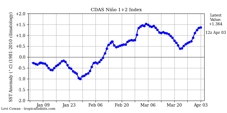


Another hurricane west of Mexico will effectively lower surface temperatures in the Nino 1.2 region.
How much is due to the volcano spewing millions of tons of water into the atmosphere?
Not much.
Jucker et al. 2023
Jenkins et al. 2023
Zhang et al. 2022
Zhu et al. 2022
From your first study.
“””This study examines the aftermath of the eruption and reveals that surface temperatures across large regions of the world increase by over 1.5°C for several years, although some areas experience cooling close to 1°C”””
That seems like a big change for SEVERAL YEARS.