Guest disalarmism by David Middleton
Do you ever watch the DIY Network? The TV network where they have all the “Do It Yourself” home improvement shows? I don’t watch it because I can’t do anything like that myself. If a home improvement or repair project is much beyond duct tape and bungee cords, I’m on the phone to a professional in a heartbeat. When I was a bachelor, the pipe under my kitchen sink was leaking. So I wrapped in in duct tape and put a bowl under it. Whenever it started to leak again, I wrapped it with more duct tape. I actually left the roll of duct tape attached to the pipe, so I could easily wrap more duct tape. When I got married and we renovated the house, the plumbers actually took pictures of my “handiwork.” Is it duct tape or duck tape? But I digress…
I may not be able to fix things around the house, but it occurred to me that if the climate (e.g. average surface temperature of the Earth) is sensitive to atmospheric CO2, there ought to be a simple DIY way to demonstrate it. So, I broke out two of my favorite data sets: Moberg et al., 2005 (a non-hockey stick 2,000 year northern hemisphere climate reconstruction) and MacFarling-Meure et al., 2006 (a fairly high resolution CO2 record from the Law Dome, Antarctica ice cores).
For the sake of this exercise, I am going to assume that the “greenhouse” warming effect of CO2 is logarithmic. While this is not necessarily a safe assumption, it’s a good bet that it is a diminishing returns function… So a logarithmic function is probably good enough for a DIY project.
The first thing I did was to crossplot the Moberg temperature anomalies against the MacFarling-Meure CO2 values…

R² = 0.0741… not exactly a robust correlation. Why is the correlation so bad below 285 ppm? Well, that’s the data from the lower resolution DSS core. What happens if we only use the data from the very high resolution DE08 core?

R² = 0.1994… Roughly a 20% explained variance… Not too shabby for noisy climate data. We also get a climate sensitivity that is in line with other recent observation-derived TCR (transient climate response) estimates: 1.23 °C per doubling of atmospheric CO2 . Note that this puts the “we’re all going to die” 2.0 °C limit out to about 720 ppm CO2 and the “women, children and poor people will die” 1.5 °C limit out to about 560 ppm CO2. So, it’s not worse than we thought, unless you’re an alarmist. Then it’s probably worse than you will believe. 1.23 °C is very close to the IPCC TAR estimate of 1.2 °C sans feedback mechanisms.
If the amount of carbon dioxide were doubled instantaneously, with everything else remaining the same, the outgoing infrared radiation would be reduced by about 4 Wm-2. In other words, the radiative forcing corresponding to a doubling of the CO2 concentration would be 4 Wm-2. To counteract this imbalance, the temperature of the surface-troposphere system would have to increase by 1.2°C (with an accuracy of ±10%), in the absence of other changes. In reality, due to feedbacks, the response of the climate system is much more complex. It is believed that the overall effect of the feedbacks amplifies the temperature increase to 1.5 to 4.5°C. A significant part of this uncertainty range arises from our limited knowledge of clouds and their interactions with radiation. To appreciate the magnitude of this temperature increase, it should be compared with the global mean temperature difference of perhaps 5 or 6°C from the middle of the last Ice Age to the present interglacial.
Things aren’t looking too good for feedback amplification.
The next thing I DIY’ed was to calculate a “CO2 temperature” using this equation:
T = 1.7714ln(CO2) – 10.305

The gray curve is the Moberg temperature reconstruction, the red dashed curve is Moberg at a constant 277 ppmv CO2. Not much difference between the gray and red dashed curves.
Let’s now apply this to the HadCRUT4 northern hemisphere temperature series (via Wood for Trees).

Northern hemisphere warming since 1979
- Total: 0.91 °C (0.01 to 0.92)
- CO2-driven: 0.33 °C (0.00 to 0.33)
- Not CO2-driven: 0.58 °C (0.01 to 0.59)
This would suggest that anthropogenic CO2 emissions are only responsible for 36% of the warming since 1979.
Let’s now look at some RCP (representative concentration pathways) scenarios.

With a 1.23 °C climate sensitivity, not even the Bad SyFy RCP8.5 exceeds the “we’re all going to die” 2.0 °C limit and RCP4.5 and 6.0 pretty well stay below the “women, children and poor people will die” 1.5 °C limit. Note than an exponential extrapolation of MLO CO2 basically tracks RCP4.5. Also note that HadCRUT4 clearly exhibits a ~60-yr cyclical variation and continued warming from the Little Ice Age (part of a ~1,000-yr cyclical variation). For those math purists who object to my geological use of the word “cyclical,” pretend that I wrote “quasi-periodic fluctuation.”
The Phanerozoic Eon
This is all well and good for the Late Holocene; but what about the rest of the Phanerozoic Eon? Thanks to Bill Illis, I have this great set of paleoclimate spreadsheets. One of the paleo temperature data sets was the pH-corrected version of Veizer’s Phanerozoic reconstruction from Royer et al., 2004. The Royer temperature series was smoothed (spline fit?) to a 10 million year sample interval matching Berner’s GeoCarb III, thus facilitating crossplotting.

Shocking!!! It yields a climate sensitivity of 1.28 °C. Royer’s pH corrections were derived from CO2; so it shouldn’t be too much of a surprise that the correlation was so good (R² = 0.6701)… But the low climate sensitivity is truly “mind blowing”… /Sarc.
References
Berner, R.A. and Z. Kothavala, 2001. GEOCARB III: A Revised Model of Atmospheric CO2 over Phanerozoic Time, American Journal of Science, v.301, pp.182-204, February 2001.
Hadley Centre. Data from Hadley Centre. http://www.metoffice.gov.uk/hadobs/hadcrut4/data/download.html Data processed by www.woodfortrees.org
Illis, B. 2009. Searching the PaleoClimate Record for Estimated Correlations: Temperature, CO2 and Sea Level. Watts Up With That?
MacFarling Meure, C., D. Etheridge, C. Trudinger, P. Steele, R. Langenfelds, T. van Ommen, A. Smith, and J. Elkins (2006), Law Dome CO2, CH4 and N2O ice core records extended to 2000 years BP, Geophys. Res. Lett., 33, L14810, doi:10.1029/2006GL026152.
Moberg, A., D.M. Sonechkin, K. Holmgren, N.M. Datsenko and W. Karlén. 2005.
Highly variable Northern Hemisphere temperatures reconstructed from low- and high-resolution proxy data. Nature, Vol. 433, No. 7026, pp. 613-617, 10 February 2005.
NOAA. Data from NOAA Earth System Research Laboratory. http://www.esrl.noaa.gov/gmd/ccgg/trends/ Data processed by www.woodfortrees.org
Royer, D. L., R. A. Berner, I. P. Montanez, N. J. Tabor and D. J. Beerling. CO2 as a primary driver of Phanerozoic climate. GSA Today, Vol. 14, No. 3. (2004), pp. 4-10
Featured image from Wikipedia.
The DIY Climate Sensitivity Toolkit
DIY Climate Sensitivity Toolkit
Duck or duct? Both – it’s made of duck cloth and can be used for ducting.
It can be used for anything! LOL!
true – but the silvery colour was intended to blend in on air-con ducting. All in Wikipedia so it must be true.
But duct tape is just like the Force:
it has a dark side, and a light side;
it is everywhere;
and it binds the Universe together
The adhesives are also intended to perform better on a heated duct. The original intent was to act as a seal at duct joints. The joints should be secured with sheet metal screws (but often are not) so the tape also acts as a mechanical load carrying feature as well.
There a numerous other variations to the ubiquitous silver tape, including some rather poor knock-offs.
In the flight test portion of my industry we also use a higher performing version we call “100-mile-per-hour-tape” because it will stay attached to the surface of aircraft in very high wind speed often exceeding 100 mph.
No, we don’t tape the wings on… only used to cover over a smallish access holes (10 mm dia) that might cause acoustic issues.
It’s the handyman’s secret weapon. – Red Green
David Middleton,
This was so informative, I love learning new things! whoda thunk that Duc(k)t tape can be used to remove warts!
It can be used to remove cactus needles… So, it should work on warts… 😉
If it moves and isn’t supposed to, duct tape.
If it doesn’t move and is suppossed to, WD-40.
Chicago in late February, the under sink area is cool (55 degrees), the cold water running thru the drain is a measured 45 degrees.
After chasing the leak with at least a quarter roll of duct tape and still having leaks, I in my desperation decided to run HOT water down the sink.
I “think” it melted the duct tapes glue, cus after compressing the tape against the “hot” pipes there ain’t a drop falling into the bowl.
I’ve got a couple friends saying it won’t last a month, we’ll see 🙂
https://www.youtube.com/watch?v=MjL6WOgwzbY
David Middleton — appreciate details on the 36% [IPCC qualitatively referred it as more than half — global], it will help readers. What about the Southern Hemisphere and global?
Thanks in advance
Dr. S. Jeevananda Reddy
.
I’ll try to work something up.
Gorilla tape is the only one I use any more. The tape works wonders.
MarkW, If it moves and is not supposed to – hammer until it stops;
If it doesn’t move and is supposed to – hammer until it does.
Georgia Chrome.
Mark W – as they (used to) say in the RN “If it moves, salute it, if it don’t move, paint it “
DM,
Anything?
The first duct tape experiment conducted by a grandson aged 4, on discovering a roll, was to try hard to seal over all orifices of the pet dog.
Geoff.
Actually it’s no good for duct work.
https://servicechampions.com/why-duct-tape-should-never-be-used-to-seal-air-ducts/
Clearly they just didn’t use enough duct tape.
Actually it’s good for just about everything *except* ducting. For metal heat ducts, you want to use aluminum tape; it won’t degrade over time like duck tape.
Only a goose would use duck tape 🙂
It is duct tape, and proper duct tape is aluminium backed with an adhesive, as it was developed to wrap around ducts, such as heating ducts. That other stuff is a brand name and synthetic cloth tape is much more common in usage nowadays. Duct tape is made by many more companies that that Duck bunch
We have Elephant tape amongst the other brands in the UK.
Here is an example of both by the King of Duct Tape–Canada’s Red Green in his Handyman’s Corner of the Red Green Show as he illustrates the “Handyman’s Secret Weapon”—-you guessed it—-DUCT TAPE!!
Here is a better episode https://www.youtube.com/watch?v=vPbubMAYN7g&t=0s&list=PLPkVeq_c4S7ZyUVD0yGu0OzWe-5qNXqvS&index=19
Why settle for an episode? The Feature Film is here:
BTW, it is “DIY”
Already fixed… without duct tape!
It didn’t stick, you need the duct tape after all. Still reading DYI 🤣
Nope, changed literally as I speak (type).
Now I should be able to figure out time differences from this, but it’s 24:30 here in the UK, I’m just in from a long shift, and I can’t be bothered.
Take a look at the three bullet table under figure 4 – either a rounding issue or a decimal point typo in the first and third bullet. I suspect the 0.1 should be 0.01 in each of those lines.
Fixed.
If it moves but shouldn’t… apply duck/duct tape.
If it doesn’t move but should… apply WD-40 and hammer.
Pretty good review of a contentious issue.
Duct vs duct tape… One of the most contentious issues of our time… /Sarc.
David, duct tape is not really recommended for use on AC ducts, use the thinner aluminum tape. Cloth duct tape does work on leaky drains for a while, sorta.
If you leave the roll attached to the pipe, it will work till you run out of tape. 😉
Gorilla tape is better…….:)
I once taught freshman human biology, tongue-tied at birth, after hearing a lecture on endocrine glands as ductless, a student wrote a good short essay on duckless glands.
Latitude
Elephant tape – even better!
I’m down to hose clamps over the duct tape, starting to look like a sad spiral of wishes vs horses.
But it is only dripping……
You make one assumption after another.
Leading to a wild guess of climate sensitivity
not worth more than flipping a coin.
We’ve got simple lab experiments
to suggest a doubling of CO2
might cause +1 degree C. warming.
What have you done,
other than mathematical
mass-turbation, to replace
that +1 degree C. estimate
with a better number?
I see no point in your article.
Because there is no point.
This is certainly not science — just
some assumptions plus
some speculation,
and a few jokes.
Always puzzling to see temperatures
in hundredths of a degree C.
— that makes absolutely no sense when the
majority of surface grids are wild guessed /
infilled because there were no thermometers !
If you have any duct tape left,
tell me where you live, so I can
come over and tape your fingers
together to prevent further typing!
Climate change blog:
http://www.elOnionBloggle.Blogspot.com
It simply takes actual observations and comes up with a number consistent with “simple lab experiments.”
This is how science is supposed to work. Rather than devising model-derived climate sensitivities 3-6 times as large as “simple lab experiments.”
Please tell me more about those ‘simple lab experiments’, because the influence of CO2 doubling in the atmosphere changes the heat conductivity of the mixture of gases very minutely, practically unmeasurable with current laboratory experiments (do not confuse heat or temperature with IR spectrum, as the cargo cultists do).
I don’t know what “simple lab experiments” Mr. Greene was referring to. That’s why I put the phrase in quotation marks.
Sorry if some of this was addressed elsewhere.
David: ‘This is how science is supposed to work. Rather than devising model-derived climate sensitivities 3-6 times as large as “simple lab experiments.”’
I disagree that this is how science should work. You are trying to estimate sensitivity using too-simplistic tools. You are not representing the system and you are unlikely to arrive at a good estimate. What about the CO2 that ends up in the ocean, for example? Or what if there is a covariate that influences both the temp and the CO2 release, such as melting of Arctic glaciers?
Other questions:
Looks like you are running regressions, but you talk about correlations. Which is it? It would help if people said what kind of test they were running.
Why do you use the data sets you do? What makes them favorites?
When you don’t account for known natural sources of variation in your data, such as volcanic eruptions and solar-geo energy oscillations, don’t you expect this to lower your R2?
Simple regressions seem like a poor representation of climate change and its forcers. There are better multivariate statistics to use on such data. This why models are used – they are the most appropriate representation of complex systems with many parameters. Even statistical, non-dynamical models would be more informative than this. (This reminds me of another “DIY science” post I just saw about the Pause, claiming the AGW crowd don’t recognize there was a slowing. I don’t know about the media, but scientists are very aware of it and find it intriguing; as far as I can tell they certainly don’t deny it.)
“This would suggest that anthropogenic CO2 emissions are only responsible for 36% of the warming since 1979.” This is based only on N Hemisphere data since 1979, so the 36% is not representative.
I must have missed something, since I don’t see how David got the percent of CO2 released that is attributable to humans.
It was a sarcastic reply to a stupid comment.
From the post:
I may not be able to fix things around the house, but it occurred to me that if the climate (e.g. average surface temperature of the Earth) is sensitive to atmospheric CO2, there ought to be a simple DIY way to demonstrate it.
Obviously, this is a simplistic model. It’s a freaking blog post that, not a peer-reviewed paper.
“CO2 that ends up in the ocean” doesn’t affect atmospheric temperatures. The causes of the CO2 release aren’t relevant to temperatures. Ultimately the degree to which CO2 causes warming and warming causes CO2 release doesn’t matter. The mathematical relationship between the two variables doesn’t care about causality.
The purpose of crossplotting two variables is to determine how well they correlate and how they vary with one another. This is generally done with a linear regression. The slope tells you how they vary with one another and the R² tells you how well they correlate with one another.
Here’s an example…
Figure 7: Cross-plot illustrating the correlation coefficient between measured asphaltene precipitation values and those predicted by the SVR model.
Firstly, both data sets are readily accessible from NOAA’s paleoclimatology database.
Secondly:
The MacFarling-Meure Law Dome CO2 record is the highest resolution Antarctic ice core drilled to date. It can clearly resolve CO2 shifts with durations of 30 years or more and possibly resolve shifts of shorter duration and it can detect shorter duration shifts, perhaps less than 10 years. It is the only high resolution continuous estimate of CO2 over the past 2,000 years that I am aware of.
Thirdly:
The Moberg reconstruction isn’t a hockey stick. Moberg went to great lengths to preserve the frequency spectrum of the temperature signal.
Furthermore, Moberg incorporated instrumental data into his reconstruction and calibrated to it. Hockey sticks simply replace the proxy data with instrumental data (Mike’s Nature Trick).
Fourthly, I don’t trust anything Mann-made.
Fifthly, I use HadCRUT4 instrumental data rather than anything touched by NASA GISS because I distrust the folks at the UEA Hadley Centre much less than I distrust the Hansen-Schmidt gang.
Whatever “known [and unknown] natural sources of variation in” the data are *in* the data. If nothing other than CO2 was driving temperature changes since 1850, the R² would be closer to 1.0 rather than 0.1994. The R² of 0.1994 tells me that about 20% of the temperature variation correlates with the CO2 variation.
From the post:
Recent radiation balance models using observational data yielded TCR’s ranging from 1.22 to 1.36 °C per doubling of atmospheric CO2.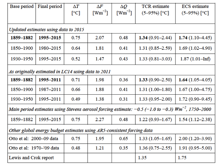
The climate sensitivity doesn’t vary regionally. The Moberg reconstruction was of the northern hemisphere. The sensitivity was calculated over the period 1850 to 1979. Oddly enough, the climate sensitivity calculated by the same method for the whole world from 520 million years ago to the “present” was 1.28 °C per doubling of atmospheric CO2.
I don’t see that in the post either. But, I actually read the post, several times. However, “the percent of CO2 released that is attributable to humans” is minuscule. It’s about 4-5% of the sum total of CO2 released to the atmosphere annually.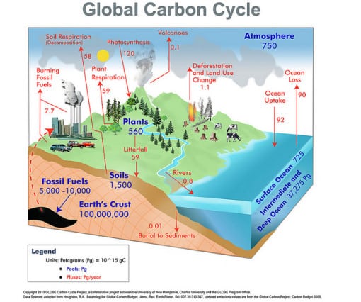
Although the human contribution mostly consists of carbon that has been released from geologic sequestration and added into the active carbon cycle. It has a cumulative effect.
David Middleton
Brilliant explanation of the finer points of your article, I just about kept up, and as a layman, I’m proud of myself!
Mr. Middleton:
A week ago I commented here,
saying that I wanted to duct tape
your fingers so you couldn’t type
another article.
I may have been “slightly”
more grumpy than usual,
as I came down with pneumonia
that day, and had been coughing
all over my computer.
I’m still not back to normal,
but I finally got back to read
your article again,
and all the comments
— including those by a very annoying
Kristi Silber, who got me riled up again.
So let me start up on you again.
It was entertaining, and brave, of you
to use humor in your article, and
then skip to tables with temperatures
in hundredths and thousandths of a degree C.
By the way, in the US the best “duct” tapes
for situations with moisture,
are Flex Tape and Monster Tape,
in my experience.
Your climate sensitivity conclusions are decent
— I believe maximum climate sensitivity
is unknown, and the percentage of warming
caused by CO2 is unknown,
so any climate sensitivity to CO2 estimate
should be presented as a whole integer
— not with one decimal place,
or even worse, the two decimal places
you used that probably impresses some readers,
but not me.
Simple lab experiments I mentioned
in my first comment,
and failed to explain for some reason,
are infrared absorption
spectroscopy (IRS)
— to determine the infrared
absorption spectrum of CO2.
That tells us CO2 is
a minor greenhouse gas,
at least in a closed system
laboratory experiment.
That’s all we really know —
everything else about CO2
is assumed, or wild guessed.
For the climate sensitivity number,
we mainly want to guess the maximum
warming if 100% of all the measured
warming after 1940 was caused by CO2.
The next step is to look at all
the global temperature data we have
— that would be weather satellite data
since 1979 — nothing else is global,
so may be inaccurate.
Climate proxy reconstructions are not
global data.
Surface temperatures are not global,
and I would argue are not even data —
they are a combination
of wild guess infilling
plus “adjusted data”
(once you change raw data
from the thermometers,
you no longer have data —
what you have is a guess
of what the data should have been
if measured accurately in the first place).
If 100% of the warming from 1979 through
2107 is attributed to CO2,
then the maximum warming
from a doubling of CO2
rounds to “+1 degree C.”
Below is a link to a 2017 study,
they fail to round off to +1 degree C.
but no one is perfect !
(Christy and McNider 2017).
https://wattsupwiththat.files.wordpress.com/2017/11/2017_christy_mcnider-1.pdf
There’s no need for tenths of a degree
— this is just a simple estimate, based
on some hard to believe worst case assumptions
about CO2 — not the IPCC water vapor positive
feedback fairy tale, but a worst case warming
assumption based on real-time global
average temperature data from satellites,
that requires very little infilling.
+1 degree C. is totally harmless — I would
say beneficial, if the main change from CO2
was warmer nights in colder, drier areas
of our planet.
I wrote a related article called
“Climate science” is missing the science:
http://www.elOnionBloggle.Blogspot.com
It is possible to get fairly precise observational estimates of the no feedbacks ECS. Using the IPCC values Monkton posted here previously, 1.16. Prof. Lindzen uses 1.2. It is utterly impossible to get ‘lab’ estimates of ECS including feedbacks. The two strongest are water vapor and clouds. Neither the oceans nor the skies can be represented in a lab experiment as you claim. Please reconsider your logic and methodology, because something is off.
OTOH, the estimates in this DIY post are likely too low. All the energy budget estimates come in with total ECS 1.5-1.8 (e.g. Lewis and Curry). IMO a ‘correct’ range because easily acheived via Bode feedback analysis with water vapor about half of what is implicit in CMIP5, and cloud feedback about neutral or maybe even a bit negative.
I think I am calculating the transient climate response (TCR) rather than the ECS from Moberg and Law Dome. Although the Phanerozoic correlation would have to be an ECS estimate.
I think the basic problem is that CO2 sensitivity is not a constant. It is temperature dependent. Think about Willis’ thunderstorm hypothesis where the negative feedback kicks in at a certain temperature. I also think this is true for CO2. At low temperatures you might get a positive feedback while at higher temperatures the feedback turns negative.
This would mean that any attempt to compute feedback would be limited to the temperature range of the period used. And, if a large range of temperature is used the feedback will average out and you end up with just the value for CO2.
Can i ask you guys a really dumb question please?
How does a CO2 molecule know where to direct the energy it absorbs and redistributes.
Presumably it’s a roundish thing, so shouldn’t energy emitted be equal in all directions, and not all directed at heating up the earth surface?
Not that I believe for a moment CO2 has more of an effect on the planet’s atmospheric temperature, never mind the surface temperature whilst it’s only, what, 0.04% of all atmospheric gases, over and above water vapour which is considerably more common in the atmosphere. As I understand it, water vapour is around 90% of greenhouse gases, and CO2 around 3%.
Sorry, I know it’s not a science class.
Oh dear.
Oh dear, oh dear.
A cross correlation between log(CO2) and temperature is established to reasonable levels of confidence (though causality is not thereby established ) certainly refuting the mythical ‘positive feedback’ and its NOT SCIENCE because it refutes what those paid to say otherwise say.
Oh dear, oh fear, oh dear….
I’m not sure if the sarcasm was necessary.
Did you not appreciate the IPCC conclusions then Richard:
-If the amount of carbon dioxide were doubled instantaneously, with everything else remaining the same, the outgoing infrared radiation would be reduced by about 4 Wm-2. In other words, the radiative forcing corresponding to a doubling of the CO2 concentration would be 4 Wm-2. To counteract this imbalance, the temperature of the surface-troposphere system would have to increase by 1.2°C (with an accuracy of ±10%), in the absence of other changes. In reality, due to feedbacks, the response of the climate system is much more complex. It is believed that the overall effect of the feedbacks amplifies the temperature increase to 1.5 to 4.5°C. A significant part of this uncertainty range arises from our limited knowledge of clouds and their interactions with radiation. To appreciate the magnitude of this temperature increase, it should be compared with the global mean temperature difference of perhaps 5 or 6°C from the middle of the last Ice Age to the present interglacial.
IPCC TAR, 2001-
The figure of 1.2C ( without feedback) is close to the result arrived at by mathematical analysis in standard textbooks such as that by Goody and not a wild guess. The guessing is most likely to come in when feedback forcing mechanisms are incorporated, and there is no reason why people should not speculate – time and further observations will decide which hypotheses have the most truth.
Mike Waite
Global temperature data
are only available since 1979:
Climate proxy reconstructions and
surface “data” are not global.
The period from 1979 through 2017
includes almost all of the warming since
1940, and includes the 2000 to 2015 period
with a flat average temperature trend.
That short period may later
appear to have been cherry picking,
and not typical — we don’t know that now
— perhaps overemphasizing warming
by including the big early 1990s to early 2000s
“step up” in the average temperature,
or underemphasizing warming,
by including the 2000 to 2015 flat trend.
The percentage of the measured warming after 1940
caused by CO2 is somewhere between 0 and 100%.
No one knows much about exact causes of climate change.
Feedback(s) are unknown.
Most of what causes climate change is unknown,
unless you are a leftist fixated on evil CO2,
and willing to claim 4.5 billion years of natural
climate change suddenly stopped in the twentieth
century, with no explanation of how, or why, that
could have happened.
The worst case Climate Sensitivity to CO2
is +1 degree C., assuming 100% of the warming
in the weather satellite era was caused by CO2
— very unlikely, but that’s just a worst case guess.
There is no need to express climate sensitivity
to CO2 in tenths of a degree C.
— that’s false precision to make an educated
guess seem like something more.
Richard, another thing that has succumbed to this post normal Dark Age is a sense of humor. On a technical note, I think this wild method reinforces the evermore evident convergence of calculations on CO2 effect toward a point of modest significance at best. Moreover, I trust you are even more dismissive of the official estimates of effect based on an even worse foundation.
Also, the “strings” and dark mass and energy of post normal physics has opened the doors wide for anything-goes science. The egregious climateering science postulates of unmitigated disaster to descend on our grandchildren may well be traceable to these untended wide open doors that let sub 100 IQs hordes into a cornucopia of new “disciplines” – grubby squatters in the once grande halls of scholarship whose ‘rights’ dare journals to deиу publication of newspeak teknickel artickles.
Gary Pearse:
“I trust you are even more dismissive of the official estimates
of effect based on an even worse foundation.”
My reply:
The IPCC is a political organization,
not a science organization,
in my opinion.
Their “predictions”,
and “95% confidence level”
are a huge pile of steaming farm
animal digestive waste products,
and I state that with 105% confidence.
Richard Greene: Your simple laboratory experiments determine the absorption cross-sections for GHGs at various wavelengths. Those are used calculate the reduction in radiate cooling to caused by a doubling of CO2, about 3.7 W/m2. If one assumes that our climate system behaves like a gray body at 288 K with emissivity 0.61, then the amount of warming at equilibrium will be slightly more than 1 K.
However, our climate system does not behave like a simple gray body. During seasonal warming, (which is 3.5 K before anomalies are calculated), the planet emits an additional 2.2 W/m2/K of LWR, not the 3.3 W/m2/K expected for a simple gray body. See Figure 1 of Tsushima and Manabe, PNAS (2013).
The “simple laboratory experiments”
that I failed to explain, for some reason,
but you realized what I meant,
only tell us CO2 has the
potential to affect the temperature …
mainly at night in cool, dry areas,
net of unknown feedbacks.
How much of an effect no one knows.
So far there is no logical reason
to assume, or wild guess, anything
other than mild, harmless warming
from CO2.
So mild and harmless, that the era
of man made CO2 in the second half
of the 20th century, had a warming period,
that looked about the same
as the warming period
in the first half of the century —
so there is no evidence
in the surface temperature
data (which I don’t trust)
that CO2 has caused ANY warming.
David,
Thank you very much for the long and detailed answer. I misunderstood a couple things.
Correlations and regressions are different. Regressions are a test of cause and effect, correlations a simple association. So the math really does make a difference when testing the relationship between variables. There are also assumptions about the data that must be met for the tests to be valid.
Looks like a signal in your data coming from natural oscillation – it’s nice and clear in spots
Regressions say nothing about cause and effect. They simply indicate the degree to which two variables are related.
R2 is the coefficient of determination, a measure of “goodness of fit.” R is the Pearson correlation coefficient, a measure of how well two variables correlate. Excel calculates R2, not R, and this is a simple DIY toolkit.
Two well-correlated variables will have higher R (absolute value) and R2 values.
Climate change is not about ambiguous anomalies, but can be boiled down to the value of a single metric. The IPCC’s self serving consensus puts this metric at about 0.8C +/- 0.4C per W/m^2 while the laws of physics put it somewhere between 0.2 and 0.3C per W/m^2 (slope of the SB curve). There’s no overlap between the IPCC’s value that was initially presumed to be large enough to justify its formation and what the laws of physics dictate it must be. The lack of overlap is why this is so incredibly controversial as the value, per the laws of physics, is too small to justify the continued existence of the IPCC and UNFCCC, thus owing to the conflict of interest at the IPCC, they will never accept the actual value.
co2isnotevil
With apologies to all the engineers out there.
It seems to me the IPCC and it’s acolytes conform to the cumulative rounding up of what I was taught in secondary school engineering as the Factor of Safety.
Calculate the structural integrity of a bridge, add in a FoS of 30%, just in case, then hand the design to the boss who adds in another FoS of 30%, just in case. Give it to the client who adds in…then the contractors, then the workforce, materials suppliers………..etc.
Engineering has come a long way over the last generation or so and is aware of this phenomenon, I don’t think climate scientists are. Worse still, at the flick of a computer keyboard, models take on a new dimension, before being handed on.
Precautionary principle gone mad.
David
I may be misreading it, but the description of Fig. 3 doesn’t seem to match the chart’s contents. Maybe it’s my browser!
“Figure 3. Moberg temperature reconstruction, “CO2 temperature”, Moberg temperature minus CO2 effect and CO2.”
The gray curve is the Moberg temperature reconstruction, the red dashed curve is Moberg at a constant 277 ppmv CO2. The orange curve is the calculated CO2-driven temperature change. The blue curve is Law Dome CO2.
dwr54, the Gray section of the chart is just EXTREMELY hard to see, it is there though if you look close enough
Here’s a version without the red-dashed curve…
I can’t help[ but note that the blip downward in CO2 levels circa 1630 comes AFTER the decline in temperatures.
I also can’t help but note that thee significant rise in temperatures which began around 850A.D. does not appear to have been preceded by ANY increase in CO2 levels. Indeed, theer appears to have been an increase in CO2 levels approximately 100 years AFTER the temperature rise.
Please explain why this is not a question mark for AGW theory when it so clearly runs OPPOSITE to what AGW says MUST happen.
Sorry for the caps, no italics available to me.
Clearly, before the late 1800’s, temperature was driving CO2 changes. This was even occurring as recently as the 1950’s.
From MacFarling-Meure et al., 2006…
David says, “Clearly, before the late 1800’s, temperature was driving CO2 changes. This was even occurring as recently as the 1950’s.”
If this is true, then it should be all the more clear the our situation is different from all that went before.
John says, “Please explain why this is not a question mark for AGW theory when it so clearly runs OPPOSITE to what AGW says MUST happen.”
AGW makes no assertions about temp changes always being the result of CO2 change or that CO2 change must result in temp change. Obviously neither of those is the case because there are other variables that influence climate.
David, yeah but you did this without solving the Navier-Stokes fluid dynamics equations. What kind of geologist are you?
So, if we are going to read these calculations correctly, the sensitivity must be read backwards since CO2 lags temperatures in your graphs. This means a CO2 increase from preindustrial to 560ppm IS CAUSED BY a <1.5C temperature increase!
Details, details… That’s why I use duct tape.
CO2 clearly lags temperature before the late 1800’s. It’s not so clear since then.
Ah! Never mind!
OK, so what changed? How did that mechanism become reversed? Data analysis is good fun, but one then sort of has to try to explain the phenomenon.
CO2 is both a cause and effect. Prior to 1850, it was almost entirely an effect. From 1850-1960, it was a bit of both. Since 1960, it’s probably been more of a cause than an effect because the atmospheric concentration is increasing at a faster rate than it was from 1850-1960.
You cannot solve Navier-Stokes, if you can you are in line for a $1 million prize!
You have your driver/driven parameters reversed. Ice Core analysis from Greenland and Antarctica all show that CO2 changes lag Earth’s temperature changes by 200-800 years on way up and 400-2,000 years on the way down. Lagging parameters are NEVER drivers of a process! As Earth has warmed since the depth of the LIA, the oceans have warmed and outgassed CO2, driving up the atmospheric concentration from ~200 to ~400. But the warming came first! Considering how terrible life was with famine, disease and death, I’m extremely glad we live in a world that is 2C warmer than circa 1550!
Bingo! And CO2 clearly has nothing to do with it, thus nothing to stop it cooling off again. But! The oceans do moderate whatever is causing atmospheric temperature changes.
Or! The long period sweep of ocean currents contains episodes where surface temps are perhaps 1-1.5C higher on average, driving atmospheric temp rise and CO2 outgassing.
Or! Arctic ocean retains heat until the surface ice breaks down, causing Arctic temperatures to become more “marine typical” until the ocean gives up sufficient heat to begin a new cycle of expanding thickness and extent. If this is the case we would never have known it until relatively recently and we have passed the minimum around 2008.
I’m taking bets on #2.
Of course, this is assuming ALL warming is due to CO2 (like Roy Spencer’s model), which is implausible… Still, an interesting exercise.
That’s what I thought going in. But, when I take the assumed CO2-driven warming, it doesn’t remove all of the warming from the signal.
OK, I see my above statement isn’t right. So I need to study this more. Again, thanks David M. Always enjoy your energy-posts.
When I started this exercise, I assumed that I was ascribing all of the secular warming to CO2. I was surprised when residual warming trends remained after I removed the calculated CO2 effect.
David, thank you for your work. Is this summary correct?
ASSUMING (for the sake of argument) that ALL global warming is due to increasing atmospheric CO2 and NONE OF IT is due to natural causes, the estimated sensitivity of climate to increasing atmospheric CO2 (“TCS”) is about 1C/(2xCO2).
That statement is consistent with Christy and McNider (2017) and also seems to be consistent with your treatise. That statement also leads to the conclusion that this alleged man-made global warming is not dangerous to humanity or the environment. Furthermore, natural variation DOES play a major role in global temperature change, so this estimate of TCS should be an upper-bound estimate of that parameter.
All good so far, EXCEPT for this observation:
The velocity dCO2/dt changes ~contemporaneously with global temperature, and its integral CO2 also varies with global temperature but LAGS global temperature by about 9 months.
http://www.woodfortrees.org/plot/esrl-co2/from:1979/mean:12/derivative/plot/uah5/from:1979/scale:0.22/offset:0.14
I suggest that the correct relationship of temperature and CO2 is as follows:
[A] There is a “base increase” of atmospheric CO2 of about 2 ppm per year, generally assumed to be from man-made causes.
[B] There is a clear signal on top of [A] that the velocity dCO2/dt changes ~contemporaneously with global temperature, and its integral CO2 also varies with global temperature but LAGS global temperature by about 9 months.
[C] The sensitivity of CO2 to temperature must be greater than the sensitivity of temperature to CO2, or the clear signal described in [B] would not exist; also, the magnitudes of both sensitivities are small and not dangerous to humanity or the environment..
Best regards, Allan
I don’t think my method ascribes all of the warming to CO2. When I subtract the calculated CO2 effect from either Moberg or HadCRUT4, some warming remains, most of the warming in the case of HadCRUT4.
Don’t forget, David, the temperatures have been fiddled to tip the slope steeper. Also, without chagning the long-term slope much, they pushed down the 1930s- mid forties peak by a fair portion of a degree to make the 1998 El Nino peak a new ‘record’.
Had they not done this, most of the degree increase since 1880 would have occurred before 1940 – in 60yrs! Temperature would then have been essentially unchanged to 2015 – a span of (Pause of) 75yrs! This period included a decline in temperature of 40 years duration that had the science community predicting the onset of glaciation – the global cooling scare (Don’t listen to the Alinsky revisionists – I lived through it all including the late 1930s!) . The fiddling took the depth of the cooling out of its notch and normalized it to be a point on a rising temperature line. Most important, it made a very low base from which the New Crisis of global warming could be measured and similarly set a 70yr high Arctic ice level as the base for measuring the decline in ice extent. Articles on the plight of seals in an iceless arctic were topical in the real global warming period up to the beginning of the 1940s. One day this will all be untangled.
You guys are probably too smart for me so correct me wherever I have erred, please.
If CO2 is upwardly sensitive to temperature-and temperature is upwardly sensitive to CO2, I think it really is way, way worse than we thought!
Can the chicken cook the egg it hatched from?
Allan
Sorry, a really dumb question.
I assume the 2ppm annual CO2 contribution to the atmosphere from man is cumulative.
So how long does a CO2 molecule hang about in the atmosphere. Is it a permanent fixture, or is it absorbed/converted/die off?
I have read it hangs about in the atmosphere for 5 years/50 years/100 Years, pick any one from three, I have no idea.
I’m now taking a slightly philosophic approach to the subject. Around the time CO2 was at it’s lowest, over the past several thousand years, it having been accidentally, and naturally sequestered, humankind happened along, alarmingly coincedentally, and discovered fire.
Since then, CO2 has risen from dangerously low levels, to levels more consistent with the planet’s survival.
An utterly amazing coincidence one can only put down to one of two things – an incredible coincidence, or divine intervention.
I’m not religious, but coincidence under these circumstances seems a step too far.
Perhaps we are being influenced, somehow, to put the brakes on CO2 production, early, assuming it is a problem, which I understand it might become over 6,000 ppm. So, very early then.
Just a thought, no scientific basis whatsoever implied. And I think I need to drain my last beer and toddle off to bed. Long day.
It’s not a matter of how long the molecule hangs around (they don’t hang around for more than about 5 years). It’s a matter of us moving molecules from geologic sequestration into the active carbon cycle.
Ah! Thank you David, now that I get, in my perverse little mind. So man happened along around the time CO2 was dangerously low, at one point I understand around 180ppm, and began to release naturally, but accidentally sequestered CO2 when he discovered fire.
I’m not religious, I just find it the most extraordinary coincidence ever. I guess the planet got lucky when we turned up.
That… And our ancestors made friends with wolves and turned them into dogs… In exchange for a pat on the head and a few scraps of food, they decided to help us hunt rather than hunt us…. Coincidence? I think not.
Not sure its the same thing. Two almost centient beings making a pact that somehow survives to this day, vs discovering fire and unwittingly affecting mankind for generations by producing a tasteless, invisible trace gas.
Almost sentient?
Hehehe…….you know what I mean.
David
So what happens to a 5 year old CO2 molecule. Does it just disintegrate?
It feeds plants, plankton and other critters that eat CO2.
David
I get that, but there seems to be this unused amount of 2ppm per year that isn’t eaten.
Which, slap me sceptical if you want, is an entirely theoretical construct.
I don’t believe anyone can measure 2ppm of anything, far less CO2, which has so many things digesting, and emitting it as both a food and by product.
HotScot – Some of the CO2 maybe cycled out of the atmosphere within 5 years, some may stay up there for 200. There is no set time a particular molecule is up there, and an average or half-life is very hard to demonstrate or calculate. It doesn’t break down like methane and other trace gases. Some is absorbed by the oceans or taken up by photosynthesis, but that’s going on at the same time the GHGs are rising – the natural sinks can’t keep up. Since the system isn’t anywhere near equilibrium, that makes it all the harder to figure out the length of time carbon stays in the atmosphere.
During each of the last 2 years the CO2 has risen 3 ppm.
Kristi
Blimey! It’s even more confusing than I thought. 😁
Thank you David for your comments on increasing atmospheric CO2. Let us assume for clarity and simplicity that your comments, effectively endorsing the Mass Balance Argument, are correct.
However David you have not responded to my primary question, repeated below.
Some more background info:
1. Let us assume that atmospheric CO2 started to accelerate strongly after about (“~”) 1940, and continues to accelerate today, due to increasing fossil fuel combustion. .
2. However, global temperature declined from ~1940 to ~1977, then increased ~1977 to ~1997, and has remained ~flat since about then, with some major El Nino spikes that have mostly or completely reversed.
So there is a correlation of increasing CO2 with global temperature that is negative, positive and near-zero – certainly NOT at all convincing that CO2 plays a significant role in driving global temperature.
Then there is this “elephant in the room” that nobody wants to discuss, that CO2 LAGS global temperature at all measured time scales, from ~~800 years in the ice core record to ~9 months in the modern data record.
The key relationship in modern data is that dCO2/dt changes ~contemporaneously with global temperature, and its integral CO2 (delta CO2 above the “base CO2 increase” of ~2ppm/year) lags temperature by ~9 months. Therefore I conclude that temperature drives CO2 more than CO2 drives temperature, and both magnitudes are quite small and not dangerous.
I wrote the paper that reached this conclusion ten years ago (January 2008) on Joe d Áleo’s icecap.us. The initial response is that I was just wrong – that it was “spurious correlation – which was false nonsense. Then somebody actually checked the math and deemed it correct, but because they KNEW that CO2 was the primary driver of global temperature then it MUST BE a feedback effect (more false nonsense).
Since then, the main response has been to ignore this huge inconsistency in the global warming mantra, because it disproves the hypothesis that dangerous global warming will result from increasing atmospheric CO2. In the last ten-years, tens of trillions of dollars of scarce global resources have been squandered on false global warming alarmism, and millions of lives have been sacrificed due to misallocation of these resources.
Properly deployed, these tens of trillions of dollars could have:
– put clean water and sanitation systems into every village in the world, saving the lives of about 2 million under-five kids PER YEAR;
– reduced or even eradicated malaria – also a killer of millions of infants and children;
– gone a long way to eliminating world hunger.
Repeating what I wrote above:
____________________________________________________
All good so far, EXCEPT for this observation:
The velocity dCO2/dt changes ~contemporaneously with global temperature, and its integral CO2 also varies with global temperature but LAGS global temperature by about 9 months.
http://www.woodfortrees.org/plot/esrl-co2/from:1979/mean:12/derivative/plot/uah5/from:1979/scale:0.22/offset:0.14
I suggest that the correct relationship of temperature and CO2 is as follows:
[A] There is a “base increase” of atmospheric CO2 of about 2 ppm per year, generally assumed to be from man-made causes.
[B] There is a clear signal on top of [A] that the velocity dCO2/dt changes ~contemporaneously with global temperature, and its integral CO2 also varies with global temperature but LAGS global temperature by about 9 months.
[C] The sensitivity of CO2 to temperature must be greater than the sensitivity of temperature to CO2, or the clear signal described in [B] would not exist; also, the magnitudes of both sensitivities are small and not dangerous to humanity or the environment..
Best regards, Allan
Much obliged Allan, although it will take me some time to digest this. However, I am aware that the temperature/CO2 relationship has been that CO2 increase follows temperature increase. What I wasn’t aware of was that the time lag has gone from 800 years to 9 months. Any suggestions as to why the time lag has reduced?
I also note that from Mona Lau (sp) graphs of increasing atmospheric CO2, the gradient seems fairly steady (although graphs are largely a mystery to me) for many years, yet we have the ‘pause in temperature rise. In fact, it appears to me, what with el ninio and la ninia, temperatures are all over the place and rising atmospheric CO2 seems the most cosistent signal amongst a lot of seemingly random temperature swings. And i realise that el ninio/last ninio are anomalies (is that the right term) and to gain a consistent temperature pattern one must allow for their fluctuations, but that seems to me to be guessing at what earths average temperature would be if they weren’t there, but they are, and they form a constituent parts of the planet’s development. So I’m at a loss as to why they are excluded (possibly not in the short term, but certainly in the long term) although I also understand that climate study is in its infancy, or at least in my opinion it is, and that emerging technology simply serves to demonstrate, with alarming regularity, more of what we don’t know, than what we do know.
And therein possibly lies the crux of my scepticism, in that I believe it incredibly arrogant of a man like Michael Mann to terrify the world with a tiny piece of evidence, then set about litigation with anyone that dares contradict him. In my experience, when someone comes out swinging punches, they have something to hide.
Finally, unfortunately, or perhaps fortunately, I find sceptics a generally positive community. We have faith in the future. And without positive people, America might not have ever been found; we might not have split the atom; flown faster than sound; developed email or invented the dishwasher. I mean, what are we scared of, getting our hands wet?
Nothing man has done on this planet, has been accomplished without endeavour and optimism. Lots of mistakes along the way, but we live in the most peaceful time in mans existence. You and I are doing something right, and all I see in the media, governments, and science, is the desire to stifle mans progression with the allure of peaceful socialism, of which, there is no such thing.
Ranting and waffling now. Sorry, you don’t deserve this. Long shift in a new job, so off to bed.
Thanks as ever for your explanations and patience.
HI Hotscot
You wrote:
“What I wasn’t aware of was that the time lag has gone from 800 years to 9 months. Any suggestions as to why the time lag has reduced?”
Not reduced – they are much different cycle periods (time durations) with corresponding different time lags.
One or more smaller cycles can exist within a larger cycle, or as Ezekiel said, “a wheel within a wheel”. 🙂
Best, Allan
_________________________
Here is a blast from the past on the same subject:
http://wattsupwiththat.com/2009/12/27/the-unbearable-complexity-of-climate-2/#comment-274521
Allan M R MacRae (01:31:52) :
Hi tallbloke (00:03:27) :
See the 15fps AIRS data animation of global CO2 at
http://svs.gsfc.nasa.gov/vis/a000000/a003500/a003562/carbonDioxideSequence2002_2008_at15fps.mp4
It is difficult to see the impact of humanity in this impressive display of nature’s power.
Still, annual CO2 concentration keeps increasing at ~1.5ppm/year – even as CO2 fluctuates by up to 16ppm/year in its natural seasonal sawtooth pattern. This 1.5ppm/year could be a manmade component (or not).
I pointed out two years ago that that global CO2 lags temperature by about 9 months in a cycle time of ~3-6 years.
We also know that CO2 lags temperature by ~800 years in a cycle time of ~100,000 years
There may be other intermediate cycles as well – Ernst Beck postulates one.
A fine puzzle for someone to sort out.
Veizer and Shaviv may have already done so.
Best wishes to all for the Holidays!
Wooded carbon sinks might have a chance of keeping up IF they weren’t constantly depleted for biofuels or for clearing at space to grow corn and Palm oil to make ethanol and other biofuels
Hey, maybe Mikey can fix his broken hockey stick with duct tape. Worth a shot.
What’s a hockey stick without lots of tape?
https://www.dickssportinggoods.com/products/hockey-tape-wax.jsp
Has a similar analysis been done looking at atmospheric co2 concentration vs co2 emissions? This might help show the strength of the natural mechanisms for co2 absorption.
Sort of. I converted the cumulative CO2 emissions to ppm and compared it to Law Dome and MLO…

Atmospheric CO2 was rising faster than emissions before 1960.
https://wattsupwiththat.com/2012/12/07/a-brief-history-of-atmospheric-carbon-dioxide-record-breaking/
You do data analysis like an unblinded experimenter.
Of course almost all data analysis is done that way.
Climate science seems to have become a bunch of unblinded experiments run by people pushing a political agenda. They are saving the world.
I don’t think that aspect of the situation gets as much respect as it deserves.
jackson
making money while claiming to be saving the world.
“climate science” is 99% politics and 1% science.
The “science” adds up to:
‘CO2 might cause some
harmless warming at night
in cool, dry areas.’
Everything else is alarmism to scare and control people,
led by virtue-signalling politicians, and the
government bureaucrats with science degrees
they hire to predict a climate crisis every year
… and then cash their goobermint paychecks.
Silence is golden
Duct Tape is silver.
If I remember correctly, not too long ago a substitute teacher was fired for following that adage.
Reminds me of my Dad’s admonishment to my brothers and me in the early 50’s: “Children should be seen and not heard”. Times have changed.
Amen to that.
A world ruled by brats.
Just what we need, but then I guess our parents said the same thing at our time of life.
Of course, this does ignore the possibility that CO2 could have nothing whatsoever with global temperatures. If the rise to the mediæval warm period was due to natural variation, and the drop into the little ice age was due to natural variation, then why cannot today’s temperatures, which are still conveniently between those two “extremes” of natural variation, also be considered natural variation?
That possibility is irrelevant to this exercise. The point here was to 1) see if a mathematical relationship existed and 2) to quantify the effect that CO2 could have on temperature. They answers were 1) yes and 2) not much.
[ For the sake of this exercise, I am going to assume that the “greenhouse” warming effect of CO2 is logarithmic. While this is not necessarily a safe assumption, it’s a good bet that it is a diminishing returns function ]
Fair enough to use it in your calculations. However, if it’s a ‘diminishing returns function’, this means that if we were to remove CO2 from the atmosphere, the ‘forcing’ per CO2 molecule goes up. What is the upper bound for forcing per CO2 molecule? IOW, at what concentration does CO2 forcing per molecule max out?
I don’t think it ever totally maxes out. However the forcing per molecule decreases with each additional molecule.
“Why is the correlation so bad below 285 ppm? Well, that’s the data from the lower resolution DSS core. “
The real problem is seen in Fig 3 – they don’t correlate. The reason is simple. You are asking how much temperature changes when CO2 changes. But you have a dataset, until 1850, where CO2 doesn’t change. So you can’t get a correlation. Temperature is changing, and CO2 is not. So T is changing for some other reason.
That doesn’t mean that temperature won’t change if CO2 changes. It just means you are looking in the wrong place. If you now come to Fig 1, the basis for the regression slope is entirely the last part of the data, post 1850, when CO2 rises above 285 ppm. And what really determines the slope is the period when the ppm rises above 310ppm, which is about 1950.
“Then it’s probably worse than you will believe. 1.23 °C is very close to the IPCC TAR estimate of 1.2 °C sans feedback mechanisms.”
The discussion here is the usual muddle of equilibrium and transient sensitivity. The slope from Figs 1 or 2 is neither. TCR would be roughly approximated if you used the slope post-1950. But that IPCC TAR estimate of 1.2, no feedback, is equilibrium sensitivity. You can’t compare a 1.23 TCR (kinda) and 1.2 ECS and say – no feedback.
“This would suggest that anthropogenic CO2 emissions are only responsible for 36% of the warming since 1979.”
No. This is, would you believe, circular reasoning. You have derived the slope from a fit to the data, T vs CO2. And then you deduce that the fitted curve is responsible for only 36%. You use no other knowledge of what it should be. In Fig 2, it is just the observation that the slope of the right part of the graph is less than the whole.
And that shows up the weakness of these datasets for the purpose. The slope relies almost entirely on the last 50 years or so when CO2 is changing. But that is when the proxy-based temperature is weakest. We know that because, per Fig 3, there is no modern rise. But we know there is. We have thermometer records, which are far superior to proxy, especially when proxies are fading out post 1950, either for lack of resolution, or they are entering the period necessarily reserved for calibration.
I think the 1.2 °C is TCR, not ECS…
https://www.ipcc.ch/ipccreports/tar/wg1/044.htm

The difference between TCR and ECS is unlikely to be noticed…
Moberg ends in 1979… Before the late 20th century warming spurt and it is very similar to HadCRUT4. The only significant divergence is from 1910-1925.
IIRC Moberg incorporated CRUTEM into his reconstruction.
David,
“Moberg ends in 1979”
And that is the problem. Most CO2 increase is since 1950, so the overlap period is about 30 years. That is all you have to try to determine sensitivity.
“The difference between TCR and ECS is unlikely to be noticed”
You need to look carefully at that diagram. TCR is the slope of the reds. They are responding to the ramp of the greens in the first 70 or so years. The forcing is the same, the TCRs are the same. The taper is in the future.
ECR comes into play after the taper, in the section they have marked with vertical green arrows. And that is where there is a big divergence. The red lags the green for a long time.
“I think the 1.2 °C is TCR, not ECS”
No, the clue is “doubled instantaneously”. CO2 doesn’t double instantaneously; they mean that they are looking at a long enough timescale that a century or so of rise could be considered so. If you look at response to a step change in CO2, you need a temperature to divide it by, to get a CS. But the T keeps increasing. The only T that makes sense is the eventual (asymptotic) limit. ECS.
Another clue is “It is believed that the overall effect of the feedbacks amplifies the temperature increase to 1.5 to 4.5°C.”. This is their standard ECS range.
If the TCR is 2 °C over 70 years and the ECS is an additional 1 °C over the subsequent 430 years, the only thing that will be noticed is the TRC. The ECS “tail” will be within the noise level of other factors affecting temperatures over such a long period of time.
NS, the datasets on temperature are so stepped on most of the effect is due to the “corrections”.
You can perfectly well do that calculation without corrections if you want. It makes almost no difference.
UAH, RSS, GISS whatever – they all show a modern rise.
I think the point of contention is how the rise since 1978 compares to the rise from 1910 to 1945. The corrections, which may very well be justified, “cool” the earlier warming period in the US.
I tend to assume that the corrections are reasonably valid.
My issue is the elimination of the instrumental records of the 1930 era warm period, and the 1945-1975 cooling trend. That sort of variability matters when doing correlation. Certainly it has warmed since 1975, but how much relative to 1938?
Hi Nick!
I have now some progress on the GHCND/GHCNM analyze.
Turns out GHCND “Daily raw” and GHCNM “Monthly raw” does NOT sum up.
Calculating ghcnm.tmax.v3.3.0.YYYYMMDD.qcu.dat “50194102000YYYYTMAX” records and comparing
with ASN00001007.dly “ASN00001007YYYYMMTMAX” records I get more or less identical TMAX values (i.e. my summarization rules work). However for this station all daily data records newer than 1995 are omitted in the “Monthly raw” file even though they exist.
I tested the following random pairs
“AU000005010” – “60311012000”
“SWM00002080” – “64502080000”
“USC00011084” – “42500011084”
“AGM00060355” – “10160355000”
What i find is a mix of unused/skipped perfectly valid daily data plus deviation between reported “Monthly raw” and calculated (from daily) raw.
It looks as if deviation depends on dsflag (data source). Different sources obviously use different algorithms.
Selected years with “random” treatment are consolidated as is, into one common “Monthly raw” file. This file is then processed with adjustments generating the qca files. Then finally the qca files are used to generate the adjusted TAVG files. Funny the TAVG files have more stations and records than the TMIN/TMAX files.
To me this does not look as a very accurate…
Have you done any comparisons on this level yourself?
“Turns out GHCND “Daily raw” and GHCNM “Monthly raw” does NOT sum up.”
Not surprising. They aren’t as related as you think. GHCND is relatively new – last decade or so. GHCNM is older; dates from big project around 1992. People collected whatever monthly records they could get and verify. They often didn’t have daily records attached. Then it was continued by NOAA based on monthly CLIMAT files submitted by met organisations. And that is what is used by the major indices. The monthly records were never assembled by GHCN adding up daily values.
You’ll need to scrutinise carefully to see if the stations are even the same. A lot of effort went into sorting out which of various records apparently representing some town or location was accepted for GHCN V3. V2 did not resolve the question, and supplied duplicates. GHCND has tried harder to be comprehensive and include everything, but it may not always match.
So you can’t expect exact correspondence, point by point. However, I doubt if any of that matters when you put together a global average.
Nick,
Maybe +/- temperature deviations does not contribute that much. I am more concerned with the skipped years.
On the cross-mapping it is difficult indeed. I used 3 iterations:
1. WMOID
2. Name + lat/long
3. Lat/long
The fourth was going to be first OK monthly raw vs calculated raw + lat/long 😎
I have to come up with something smarter (like rounded values and series) or stick with the stations I find with steps 1 to 3.
Can I ask how you treat stations with long series with few or no measurements during your selected anomaly base period?
MrZ,
“Can I ask how you treat stations with long series with few or no measurements during your selected anomaly base period?”
This is the essential feature of the least squares that I (and now BEST) use. The anomalies are first formed with no base period. A linear statistical model which includes both station offsets and a global time series is used. The requirement that the global average has time average zero over 1961-90 is then enforced as a single constraint. It is not required for individual sites.
There is an example here which demonstrates some of the issues involved.
Thanks Nick,
Your math is on another level than mine… 😎
Would an acceptable alternative be to grid the stations? I can than compare between GHCND and GHCNM using positions rather than specific stations.
1. Grid cells are formed as km away from Long/Lat 0.0.
2. A group of stations would form a monthly anomaly trend for the grid cell they’re in and missing measurements could simply be skipped, as they are instead covered by step 3.
3. For cells and years/months with missing data I would take the average from surrounding cells. This is accomplished by itterating across larger and larger grid cells until hit. Compare plotting the cells with water color and bleeding between the cells.
This process should bring me very close to where you are. When I compared USHCN processing like above with NOAA results it looks more or less identical.
The scatter in the temperature data while CO2 was constant is extremely useful: It quantifies natural variability in climate at constant CO2. It would better define a 95% ci for the slope – if David had bother to calculate one. Just using your eye, it’s easy to see that this confidence interval is sizable.
Yep
I got about 0.7 C for 2XCO2 using 250 years of HadCET data. Methodology is in the description below the graph. The two biggest variables are the cyclic AMO and the Sun. CO2e comes in a distant third.
HadCET is a pretty clean dataset – difficult for Hadley to justify adjusting the historic data. Recent years may have been affected by UHIE issues as urbanisation creeps closer to the baseline stations.
Northern hemisphere warming since 1979
AMO driven: >50%.
Sounds reasonable to me.
If, as it appears, carbon dioxide changes lag temperature changes during both long and short time periods then either carbon dioxide is and effect not a cause or it has endochronic properties far greater than those attributed to resublimated thiotimoline.
David: interesting work. May have some technical problems. The is now layer that fell in exactly 2000 years ago did not trap a sample of atmosphere as it existed exactly 2000 years ago. Air diffuses between the particles of snow for many years after snow fell 2000 years ago, before the 2000 years ago snow becomes ice with air bubbles cut off from the atmosphere. At Vostok (where accumulation is slow), 2000 year old ice contains roughly 1000 year old atmosphere. At faster accumulating sites, the lag is less. Today, climate scientist refer to an ice date and a CO2 date for for each layer. Did you use the right dating system for this project, the CO2 date?
That’s why I rely on the DE08 core when comparing CO2 to high resolution temperature data: The lag is short and accumulations rate is high. The MacFarling-Meure time series is a 20-yr spline fit of the gas age.
David: Thannks for the figures. We know from Keelling that CO2 was about 320 ppm in 1960. According to your Figures, the air trapped the 1960 layer of snow continued to mix with the atmosphere for the next several decades and with air trapped in the 1959, 1958, 1957, etc layers below. So the 1960 layer might have trapped air containing 330 or 340 or 350 or 360 ppm CO2. So the temperature in 1960 will APPeAR be due to more than 320 ppm.
I don’t think the mixing is uniform. The rule of thumb is that the resolution is 2x the sealing period. This would lead to a gas distribution of about 10 years in the DE08 core. But the distribution could be as long as 30 yr.
So, your data point for the temperature in 1960 and CO2 in 1960 likely will use a value for CO2 much higher than Keeling reported unless you how found a way to correct for this problem. Even if you have found a way to correct, the best way to correct may be controversial.
It would likely use a CO2 value that was too low, if the 1960 value was a raw ice core measurement. They use similar signal processing methods as we do with seismic data to improve resolution (eg deconvolution).
The 1960 “gas age” would be an average of at least 10 years (1950-1960), possibly as long as 30 years (1930-1960). Although, I think the most recent values are from snow pit and air flask measurements. It matches MLO fairly closely from 1958-2004. The MacFarling- Meure time series extends up to 2004, but the most most recent ice ages were considerably older. So 1958-2004 is not representative of the overall resolution of the ice core.
David: The gas is always younger than the ice that contains it. The 1960 layer must contain more than 320 ppm, unless corrections have been made. You need to look carefully at the data you used above.
The time series uses the gas age and CO2 concentration, not the ice age.
The 1969 gas layer is in the 1939 ice layer. It’s a mixture of at least the 1959-1969 gas, possibly as much as 1939-1969 gas.
Finally! Thanks for your patience. “1969 dated gases are found in 1939 ice makes perfect sense to me and eliminates some concerns.
I had to be patient with myself to finally grasp the concept… LOL!
David: It can be useful to convert CO2 into log2(CO2). 256 ppm becomes 8.00. 512 ppm becomes 9.00. The difference is 1.00 in log2 units – 1.00 doubling. With Temp on the y-axis and log2(CO2) on the X-axis, the slope is K/doubling..
The other thing you slope need is a confidence interval, usually 95%. If your slope were 1.3 +/- 0.5 K/doubling, it wouldn’t be inconsistent with the IPCC’s value of 1.8 +/- ? For the IPCC models. Technically, you need to worry about autocorrelation in the temperature data.
David: Continuing on confidence interval. The scatter in the temperature data for CO2 at pre-industrial levels of CO2 is due to natural variability in climate at constant CO2. This scatter widens the confidence interval in your slope – as it should. To properly account for natural variability, you MUST include a confidence interval. Your conclusion that 30% of warming needs to be 30 +/- X% and X might turn out to be 100%.
X probably is very high.
If X could be 90%, you haven’t invalidated the IPCCs claim that 100% of warming is likely due to man