by Andy May
Introduction
In 2014, Dr. Michael Connolly and Dr. Ronan Connolly posted three important, non-peer reviewed papers on atmospheric physics on their web site. These papers can be accessed online here. The papers are difficult to understand as they cover several fields of study and are very long. But, they present new data and a novel interpretation of energy flow in the atmosphere that should be seriously considered in the climate change debate.
By studying weather balloon data around the world Connolly and Connolly show that the temperature profile of the atmosphere to the stratosphere can be completely explained using the gas laws, humidity and phase changes. The atmospheric temperature profile does not appear to be influenced, to any measurable extent, by infrared active gases like carbon dioxide.

Figure 1, source Connolly and Connolly.
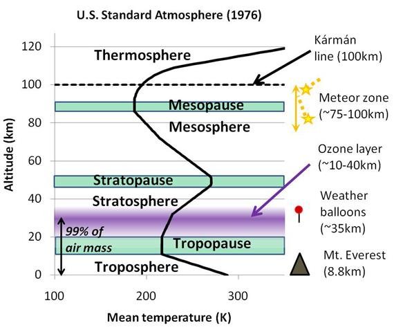
Figure 1 shows the “U.S. standard atmosphere.” The black curve is the standard atmospheric temperature as a function of altitude (Y axis). There are several key points that are important for this post. First, notice that the temperature decreases with altitude in the troposphere, then goes vertical in the tropopause, then it reverses course and increases in the stratosphere. Since we are discussing weather balloon data in this post, we are only concerned about the curve to about 35 kilometers. This region contains about 99% of the atmospheric mass. We will also be discussing the ozone layer, which is at the very top of our layer of investigation.
They evaluate available weather balloon data in terms of molar density and pressure. They find that, above the boundary layer (roughly the surface to 2 kilometers, the atmospheric layer that contains most of our weather), the trend of molar density and pressure is a line until the tropopause is reached. Above the tropopause it is also a line, but with a steeper slope, see figure 2. In figure 2, pressure increases to the right and altitude decreases to the right. Above the tropopause molar density decreases more rapidly with pressure, this suggests a change in the equation of state for the atmosphere above the tropopause. Region 3, the boundary layer, shows much more variability than the higher regions of the graph. This variability is due to changes in humidity and precipitation.
Multimers
A change in the equation of state in the atmosphere means that it will respond to external forces (“forcings”) differently. For the atmosphere, the equation of state is the ideal gas law, modified to account for factors that affect real gases, but not ideal gases. These include varying specific heat capacity, Van der Waals forces and compressibility effects among others. While the molar density versus pressure plots, like figure 2, strongly suggest that the equation of state has changed above the tropopause it does not tell us exactly what happened. Connolly and Connolly think that oxygen and nitrogen multimers form in and above the tropopause (see figure 3). Multimers are called trimers if they contain three molecules and tetramers if they contain four.

Figure 2, after Connolly and Connolly (2014) paper 1.

Figure 3 (source Connolly and Connolly, 2013)
This suggests that the atmosphere above the tropopause has a lower molar density, at a given pressure, than the tropospheric trend would suggest. The atmospheric composition and humidity above and below the tropopause are nearly identical, so composition is not the cause of this change.
The formation of oxygen and nitrogen multimers is a state change that can be called a phase change. If multimers form in the tropopause, they release the energy of formation to the surroundings. This may increase the temperature of the surroundings. The larger multimers have more degrees of freedom than the diatomic monomers (for example O2) and every additional degree of freedom increases the internal energy of a mole of multimers by ½RT. R is the universal gas constant and T is temperature. This is described in more detail in Connolly and Connolly, paper 2, section 2.2. In their section 2.2, the heat of formation (or enthalpy of formation) of the multimer is designated as ΔH. The molar enthalpy (H) of a gas is defined as,
H = U + PV … (1)
Where U is the internal energy of the gas, P is pressure and V is the volume.
U = ½αRT … (2)
The internal energy of the gas is equal to ½ of the degrees of freedom (α) times the gas constant (8.3145) times temperature (T). Degrees of freedom of a gas are defined here as the number of independent ways a gas can have energy. This includes translation, rotation and vibration. Internal energy is the sum of the energy in all the degrees of freedom of the gas. If ΔH is set to zero for a diatomic monomer, it is 4RT with 34 degrees of freedom (α) for a tetramer, according to table 2 from Connolly and Connolly paper 2. So, the heat of formation of a multimer can be significant and will affect the temperature of the tropopause and stratosphere. The formation of oxygen multimers probably involves the emission of microwave radiation.
In the tropopause, the lapse rate is near zero, this means, according to Connolly and Connolly, that the increase in internal energy, due to multimer conversion, is balanced with the loss of thermal energy converted to potential energy, due to gravity, at this altitude. I realize that thermal energy can be defined in different ways, but here we define it as the internal energy of the gas due to its temperature. As altitude increases and we enter the stratosphere, either more multimers are formed or they get larger and internal energy increases more rapidly than thermal energy is converted into potential energy and the air temperature begins to increase. In the troposphere, there are no multimers and thermal energy is transformed into potential energy as the altitude increases and the air temperature steadily decreases (the “lapse rate”). This causes the slope change shown for region 1 (tropopause and stratosphere), seen in figure 2.
Ozone
Ozone concentration starts to increase with altitude in the stratosphere as well. The classical explanation for the formation of ozone is called the Chapman mechanism and it is illustrated in figure 4. Chapman hypothesized that ultraviolet light (UV) striking oxygen molecules will split them into individual oxygen atoms. He then speculates, that some of these would combine with nearby oxygen molecules and form ozone.

Figure 4 (source Connolly and Connolly, 2013)
There are several problems with the Chapman mechanism. First, it requires a great deal of energy to break a diatomic oxygen molecule’s bonds. Further, if the Chapman mechanism were the only mechanism forming ozone, why would ozone concentrations, in the Northern Hemisphere, be the highest in the Arctic in the spring? The equator (the red line in figure 5) receives the most UV from the sun, yet the ozone concentration there is much less than in the Arctic, the dark blue line in figure 5. Further, one would think that the Arctic and Northern Hemisphere ozone concentration would peak in the summer, yet it peaks in the spring and falls in the summer, and begins to increase in the winter. The Chapman mechanism also has other flaws as documented here.
According to classical theory, the extra energy in the tropopause and stratosphere that reverses the negative lapse rate seen in the troposphere, comes from “ozone heating.” Ozone absorbs UV light from the sun and radiates heat which warms the tropopause and stratosphere. Yet, the tropopause stays in place during Arctic and Antarctic winters when there is no sunlight. Given these contradictions, Connolly and Connolly came up with an alternative mechanism.

Figure 5 (source Connolly and Connolly, 2014, paper 2)
Ozone formed directly from oxygen multimers also requires UV radiation, but it requires much less than is required in the Chapman process. Figure 6 shows the process described in Connolly and Connolly (2014). There a multimer of eight oxygen atoms and four oxygen molecules is transformed into two ozone molecules and one regular oxygen molecule. This process requires sunlight and abundant multimers to work, but less energy. Further, the formation of the multimers, themselves, can occur without sunlight and the formation process releases heat of formation, which helps form the tropopause and warms the stratosphere.

Figure 6 (source Connolly and Connolly, 2013)
Their idea allows ozone to form more easily and with less energy and it provides additional energy during the Arctic and Antarctic winters when there is no sunlight for months. The idea that multimers make ozone easier to form, is only one of the potential impacts of possible multimer formation in the tropopause and stratosphere. Multimer formation may also influence tropospheric weather as discussed in Connolly and Connolly paper 2.
The Weather balloon data
Weather balloons record temperature (T), pressure (P) or sometimes altitude (h), horizontal wind speed and direction, and relative humidity. Relative humidity is converted into absolute humidity using the temperature. There have been one to four launches a day from about 1,000 stations around the world – in some cases since the 1950s or earlier. That is about 13 million datasets containing data from the ground to the mid-stratosphere (~30-35km altitude). A weather balloon launch in Chile is shown in figure 7.

Figure 7 (Weather balloon launch in Chile, source: European Southern Observatory)
Nobody had analyzed the weather balloon data in terms of molar density before, but it is quite straightforward to do. Molar density, D = n/V = P/(RT) (where R=8.314, is the universal gas constant). So, all you need to do is divide the P (Pressure) values by the corresponding T values (multiplied by 8.314). The units of “D” are moles/m3.
From a climate perspective, it is better to view the molar density versus pressure plot in terms of temperature and height as in figure 8. To compute temperature, we first have to compute best fit lines to each region of figure 2 to obtain slopes and intercepts. Connolly and Connolly call the slopes “a” and the intercepts “c,” such that:
D = aP + c … (3)
Therefore, since D = P/(RT) and using the ideal gas law:
 … (4)
… (4)
“R” is still the ideal gas constant equal to 8.3145 J/(mol.K). The coefficients, “a” and “c,” are not constants and vary from place to place. Typical a and c coefficients are shown in table 1. In figure 2, the “humid” phase in table 2 is region 3, the “light” phase is region 2 and the “heavy” phase is region 1 or the tropopause and stratosphere. A spreadsheet for computing temperature from the coefficients, using equation 4, is in the supplementary materials for Connolly and Connolly, paper 1. In table 1, there are two entries for the near Artic Norman Wells site. One is for the ground (g) and other is for the tropopause/stratosphere (u). Near the poles the heavy phase (multimer formation) can occur near the ground.

Table 1, from Connolly and Connolly, paper 1.
Using equation 4 and the coefficients of the best fit lines, like those in table 1, we can estimate temperature (T). This has been done in figure 8. Most of the balloon launch sites can be fit with two or three best fit lines. In figure 8, both are fit with three lines. Lake Charles, Louisiana is sub-tropical and the boundary layer requires a separate fit due to high humidity. Norman Wells, Northwest Territories, Canada requires three because the boundary layer, in winter time, can show a phase change very like the phase change observed in the tropopause. This might be due to the formation of multimers at the surface.

Figure 8, after Connolly and Connolly, paper 1
The boundary layer is defined, in the papers, as where the absolute humidity is greater than one gram of water per kg of air. This is roughly greater than 0.1%. As figure 2 shows, the slope is relatively more variable in this region (region 3). Changes in temperature, humidity and precipitation affect the slope in this region. The boundary layer may not exist in the Arctic and Antarctic in winter, where surface humidity can be very close to zero in cold weather. Yet, slope anomalies exist there as well, sometimes going the other way as seen in the Arctic (figure 8B). These Arctic and Antarctic winter anomalies look suspiciously like the tropopause anomalies.
Connolly and Connolly found that there is a change of state, that might be a phase change, at the top of the troposphere and a similar change occasionally at the surface, in the polar regions, in the winter. After accounting for this apparent phase change, they could describe the atmospheric temperature profiles of all ~13 million weather balloons entirely in terms of the thermodynamic properties of the bulk gases and humidity. For the Earth’s atmosphere, the bulk gases are N2, O2, argon and sometimes H2O. By “thermodynamic properties”, they mean the gas laws, the role of gravity, changes in state (i.e., phase changes), differing heat capacities, etc. Of the four bulk gases, only H2O is infrared-active and the influence H2O has on the atmospheric temperature profile has nothing to do with its infrared activity. Instead, it is related to its phase changes and the fact that it has a higher heat capacity than the other bulk gases.
The temperature fits did not require consideration of the CO2 concentration or any of the other infrared-active (“IR-active”) gases. If the effect of CO2 and other greenhouse gases were as strong as predicted by the climate models, one could reasonably expect that they would affect these temperature profiles.
Most versions of “the greenhouse effect” theory argue that the infrared activity of greenhouse gases (“GHG”) alters the atmospheric temperature profile. In particular, the models suggest that as carbon dioxide is added to the troposphere by man’s emissions, the troposphere should warm. This is supposed to be counteracted by increasing the speed of cooling. Thus, they predict that the troposphere warms and the stratosphere cools due to man’s carbon dioxide emissions changing the atmospheric temperature profile. Therefore, a debate exists over whether there is a “tropospheric hotspot” signature from GHG warming. Some also argue that there must be “stratospheric cooling.” But, the key to these theories is that the IR activity of the GHGs is supposed to in some way alter at least some part of the atmospheric temperature profile. This IR-based effect is the greenhouse effect. But, if the IR activity of the GHGs doesn’t influence atmospheric temperatures, as the Connolly’s found, then there isn’t a greenhouse gas greenhouse effect!
As mentioned above, their analysis of molar density versus pressure reveals a change in slope, probably due to a phase change, that occurs above the troposphere. This phase change can explain most, if not all, of the changes in temperature behavior associated with the tropopause and stratosphere. The tropopause and stratosphere are treated as distinct regions from the troposphere because they have different temperature behaviors than the troposphere. That is, the lapse rate approaches zero in the tropopause and becomes positive in the stratosphere. While this is true, the tropopause and stratosphere share the same molar density vs. pressure slope, intercept, and equation of state.
Multimers and the Ozone Layer
In Connolly and Connolly’s paper 2, they argue that the phase change identified in their paper 1 is due to the formation of oxygen (and possibly nitrogen) multimers, i.e., (O2)n, where n>1. The formation of multimers in the atmosphere is not a new idea and has been studied by Slanina, et al., 2001.
They also noted that if multimers are forming in the tropopause and the stratosphere, there is an alternative mechanism for the formation of ozone, which is much more rapid than the standard Chapman mechanism. That is, ozone (O3) could form directly from the photolysis of oxygen multimers, for example, a trimer (three linked O2 molecules) of oxygen could dissociate into two ozone molecules: (O2)3 + uv light → 2O3.
There is a remarkable correlation between the proposed phase change conditions and ozone concentrations, see figure 9. This is consistent with the Connolly’s mechanism for the formation of ozone, and suggests that the ozone is generated rapidly in situ. Table 2 lists the computed phase change conditions for 12 different regions, separated by latitude, around the world:

Table 2, Source: Connolly and Connolly paper 2

Figure 9, Source: Connolly and Connolly paper 2
Figure 9 shows the monthly variation of the optimal phase change pressure for several of the regions versus ozone formation (from NASA’s Total Ozone Mapping Spectrometer) for the same region. The correspondence between them is clear. It is interesting that the optimal pressure conditions for the phase change vary dramatically from month to month in each latitude band in figure 9 and that the level of ozone also varies dramatically from month to month. This suggests that ozone creation is very fast in the upper atmosphere, something that is consistent with the Connolly’s hypothesis, but not consistent with Chapman’s. It is also not consistent with the hypothesis that chlorofluorocarbons destroy the ozone layer, but that is another story.
Local Thermodynamic Equilibrium
Connolly and Connolly have shown, using the weather balloon data, that the atmosphere from the surface to the lower stratosphere, is in thermodynamic equilibrium. They detected no influence on the temperature profile from infrared active (IR-active) gases, including carbon dioxide. This is at odds with current climate models that assume that the atmosphere is only in local thermodynamic equilibrium as discussed by Pierrehumbert 2011 and others.
Climate models split the atmosphere vertically into many different layers, each a few kilometers thick, then the layers are broken up geographically into grid boxes. Each grid box is assumed to be in local thermodynamic equilibrium (LTE). These boxes are assumed to be thermodynamically isolated. However, within each grid box, the total energy content is assumed to be completely mixed. Because each box is isolated from the surrounding boxes, the rates of IR emission and absorption from the box are a function of:
-
The IR flux passing vertically through the box
- The current average temperature of the box
-
The concentrations of each of the IR-active gases in the box
Since they are thermodynamically isolated from each other, if a grid box absorbs more (or less) IR radiation than it emits, this will alter the energy content and average temperature of the box. For this reason, a grid box can develop an energetic imbalance relative to the surrounding grid boxes through radiative processes. Therefore, in the models, the presence of “greenhouse gases” (e.g., CO2) alters the underlying atmospheric temperature profiles. But, is this LTE assumption valid? So far, it has simply been assumed to be the case.
What would happen if the grid boxes are not thermodynamically isolated? Well, if one grid box becomes “hotter” or “colder” due to radiative heating/cooling than the surrounding boxes, then energy would flow between the neighboring grid boxes until thermodynamic equilibrium was restored. If the rates of energy flow are fast enough to maintain thermodynamic equilibrium then the radiatively-induced imbalances from the IR-active gases would disappear. Instead, the atmospheric temperature profile would be determined by the thermodynamic properties of the bulk gases. This is what Connolly and Connolly found was happening.
With thermodynamic equilibrium, we would still expect to see, the often observed, up-welling and down-welling IR radiation. We would also still expect the total outgoing IR radiation to remain roughly in balance with absorbed incoming solar radiation, as we currently observe. And, we would expect the IR spectrum to show the peaks and troughs characteristic of the main IR-active gases, i.e., H2O, CO2 and O3. However, Connolly and Connolly found that the IR-activity of these gases does not alter the atmospheric temperature profile.
Pervection
The standard mechanisms for energy transmission within the atmosphere usually considered are radiation, convection (of which there are three types: kinetic, thermal and latent) and conduction. Because air is a poor heat conductor, conduction’s role in atmospheric energy transmission is negligible. That initially would appear to leave just radiation and convection. Both radiation and convection move thermal energy slowly, too slowly to keep the atmosphere in thermodynamic equilibrium. However, we know from thermodynamics that thermal energy can be converted to work and transmitted and then turned back into thermal energy. Thermal energy transfer is not the only method of energy transfer at work in this equilibrium process.
Connolly and Connolly found that there is almost no experimental data on the rates of vertical convection outside of clouds and above the boundary layer. But, from the limited data they have, the rates of vertical convection appear to be too slow to maintain thermodynamic equilibrium from the surface to the stratosphere.
They found an additional energy transmission mechanism which seems to have been neglected, “through-mass” mechanical energy transmission. Unlike convection where the energy is only transported by a moving air mass, this mechanism allows mechanical energy to be transmitted through the air mass without the air itself having to move significantly. This is like conduction, except that conduction involves the transmission of thermal energy, while this mechanism involves the transmission of mechanical energy. To distinguish it from “convection” (which comes from the Latin for “carried with”), they use the term “pervection” (from the Latin for “carried through”). In this process, molecules collide transmitting mechanical energy to one another. An analogy would be a long tube filled with ping-pong balls and the tube is only wide enough for one ball. If a ping-pong ball is forced in one end of the tube, one will immediately be forced out the other end. None of the ping-pong balls move very far, but the energy is quickly transmitted, mechanically, a long distance.
In Connolly and Connolly paper 3, they designed a series of controlled experiments to try to quantify the relative rates of energy transmission of each of these mechanisms in air. Their experiments showed that, at ground level, energy transmission by pervection (aka “work”) is several orders of magnitude faster than conduction, convection or radiation! This then explains why the troposphere and stratosphere are not thermodynamically isolated, as the climate models assume.
Pervection is a mechanical energy transmission mechanism, not a thermal energy transmission mechanism, in common thermodynamic terms it can be considered “work.” Mechanical and thermal energy can be converted to one another as thermodynamics teaches us. So, either energy transmission mechanism can, and will, act to restore thermodynamic equilibrium. This also highlights why it is important to consider multiple types of energy and energy transmission mechanisms.
Conclusions
The three papers by Connolly and Connolly provide new data and analysis that show the IR-active trace gases in the atmosphere have an insignificant effect on the atmosphere’s vertical temperature profile. They show the atmosphere, at least to the lower stratosphere, is in thermodynamic equilibrium which invalidates the local thermodynamic equilibrium assumption used by the global climate models.
Unlike other critiques (Jelbring, 2003, Johnson 2010, O’Sullivan, et al. 2010, Hertzberg, et al. 2017, and Nikolov and Zeller, 2011) of the carbon dioxide climate control knob hypothesis (Lacis, et al., 2010), this analysis explains two lines of evidence often used to justify the carbon dioxide greenhouse effect:
-
Why is the lapse rate positive (temperature increasing with height) in the stratosphere?
- Why do we observe both upward and downward traveling IR radiation in the atmosphere?
The lapse rate, which averages about -6.5°C per kilometer in the troposphere, goes vertical and eventually reverses sign in the tropopause and stratosphere due, at least in part, to the formation of multimers according to Connolly and Connolly. The formation of multimers releases energy, which can account for at least some of the tropopause and stratospheric heating. IR-active atmospheric gases like water vapor and carbon dioxide do radiate IR in all directions and this can be detected, it is just that this radiation does not affect the atmospheric temperature profile significantly according to Connolly and Connolly’s work.
It takes less energy to form ozone directly from oxygen multimers than from splitting diatomic oxygen molecules, although both require UV light. Further, ozone formation does correlate well with the conditions required for multimer formation. Multimer formation does not require sunlight and can occur at night. Also, ozone concentrations in the ozone layer vary rapidly, suggesting ozone is created and destroyed monthly. This is inconsistent with the Chapman process.
The key problem with the conventional idea of IR-active gases, like carbon dioxide, influencing atmospheric temperatures is the concept that the atmosphere is only in local thermodynamic equilibrium. The weather balloon data strongly suggest that the atmosphere is in thermodynamic equilibrium, meaning IR-active gases have little to no influence on atmospheric temperatures. For this to be true a very fast energy transfer mechanism must be at work. Connolly and Connolly suggest that this transfer mechanism is mechanical in nature. Using thermodynamic terminology, the mechanism is “work.” They have proposed a name for the mechanism and call it “pervection.”
Currently, the multimer formation in the tropopause and stratosphere is speculative and requires experimental verification. Likewise, the details of forming ozone from oxygen multimers need to be worked out and documented. Pervection is a proposed name for a relatively obvious form of energy transfer that we observe all the time and has just been overlooked for some reason in climate science. Air is compressible, of course, but it does transmit mechanical energy. BB guns, air compressors and inflatable tires wouldn’t work without this energy transfer process.
So, clearly the Connolly and Connolly ideas need further work, but they have put together a very coherent and detailed hypothesis that deserves serious consideration. It is, at least, as well documented and supported as the conventional carbon dioxide greenhouse theory.
For those that want to read a more detailed summary of the Connolly’s work that includes a description of their laboratory work, I refer them to the Connolly’s summary here and to their three papers, linked at the top of this post.
My views on the Nikolov & Zeller papers
Like Anthony, seaice1 & Dr. Strangelove, Roy Spencer and many others who have commented here and elsewhere, I agree that Nikolov & Zeller’s papers don’t warrant their conclusions (or the categorical press releases that accompanied it). I agree that their analysis is consistent with their claim that there is no CO2 greenhouse effect. It is also consistent with our analysis. However, as Roy Spencer and others have repeatedly demonstrated, it is also consistent with there being a greenhouse effect.
Being consistent with a theory is not a proof of that theory, especially when it is also consistent with conflicting theories!
As seaice1 points out, their analysis is in many ways simply a curve-fitting exercise. Moreover they only used 5 points for their fitting and there is some subjectivity in the exact values they used for those 5 points.
Also, as Matthew R Marler points out in his August 22, 2017 at 3:07 pm comment, and as Andy summarises in the post, the upward and downward transmission of IR radiation in the atmosphere with characteristic CO2 and H2O peaks has been repeatedly observed experimentally, yet Nikolov & Zeller offer no explanation for this.
That said, I do think Nikolov & Zeller’s idea of using observations from other celestial bodies in the Solar System is a good one. It’s just that their analysis is not as conclusive as they claim.
Ronan,
Not only does the Nikolov and Zeller analysis fit multiple observed extraterrestrial atmospheres but it also fits what we would expect to see from an application of the gas laws. Why do you think that is insufficient?
I have told Ned Nikolov that he is just restating old knowledge from the days before the radiative greenhouse effect came to dominate climate science.
Stephen, N&Z’s hypothesis is incomplete and needs to be fleshed out. They need to be able to explain the structure of the atmosphere, especially the troposphere/tropopause/stratosphere portion. They also need to explain the characteristics of the upward and downward radiation spectra. To me, these are the weaknesses in their ideas and also the ideas of the dragon slayers. None of them are saying anything all that wrong, their ideas just are not fully fleshed out. Plus, sometimes they put up strawmen (stuff not said by their opponents, but easy to argue against) and then shoot them down. However, they aren’t the only group that does that – their opponents and the alarmists often do that also.
In my exchanges with N, I take it as he thinks that all takes place below the surface of last emission. My argument with that is if you want surface temp, you have to account for work being done by the atm. Him, “that’s all part of the vapor pressure defined by gravity, and therefore temp”, or something like that.
Ned doesn’t try to explain the structure of the atmosphere and doesn’t need to for his basic hypothesis.
However, I can explain that structure.
For an atmosphere to be retained long term it must always be successful in balancing the downward force of gravity with the upward pressure gradient force which latter force is caused by kinetic energy at the surface acting on the weight of the gases above.
If you then get variations in layers caused by different radiative characteristics within each layer then the atmosphere uses convection to return to hydrostatic equilibrium.
So, the lapse rate from surface to the boundary with space must always average out at the slope set by mass and gravity and distortions in one layer will come to be offset by an equal and opposite distortion in another.
You will see that Earth’s lapse rate structure forms a sideways ‘W’ shape with temperature declining with height in the troposphere and mesosphere but increasing with height in the stratosphere and thermosphere.
If one were to average out the slope across all four main layers then the slope must match that determined by mass and gravity for long term hydrostatic equilibrium.
There is no other solution if an atmosphere is to be retained. Otherwise the atmosphere would either float off into space or fall to the ground depending on the sign of any net imbalance.
Convection always adjusts to neutralise radiative imbalances.
On our multimerization theory
As we discuss in Section 2.2 of Paper 2, we agree with Dave’s August 22, 2017 at 6:41am comments that while nitrogen and oxygen dimers are found at very low temperatures and laboratory pressure, these conditions are not comparable to the temperatures and pressures found in the tropopause/stratosphere (although, I don’t know why you refer to them as “telomeres” – aren’t telomeres those bits of DNA at the ends of chromosomes?)
We also pointed out in the same section that the solid “red oxygen” tetramer (which Dave mentions in a few comments) only occurs at very high temperatures and pressures. So, as Dave says, it is not relevant for the temperatures/pressures of the tropopause/stratosphere.
Also, while oxygen dimers (a dimer = a multimer of size N=2) have been observed in the atmosphere spectroscopily and have been considered both theoretically and computationally, they are only found in trace amounts. So, we don’t believe oxygen dimers can explain the phase change.
However, from our quite detailed literature review, we didn’t find any groups that had considered or checked for the possibility for the formation of (non-dimer) multimers occurring under the temperatures/pressures of the tropopause/stratosphere.
As Dave has pointed out, the phase diagrams for oxygen and nitrogen are fairly well characterized experimentally at both low T/high pressure and high T/high pressure. But, it turns out that the low T/low pressure conditions of the tropopause/stratosphere haven’t been well-studied.
Telomer is defined in chemistry as a small polymer. It is also used for the short bits at the end of the DNA molecule in contrast to the long bit of DNA which is a polymer.
Please see wikionary Telomer -an extremely small polymer one whose degree of polymerization is between 2 and 5.
It is a standard chemical term why do you not seem to know it?
In biology, the feature you mention is actually called a telomere, ie, a region of repetitive nucleotide sequences at each end of a chromosome, which protects them from deterioration or from fusion with neighboring chromosomes. .
In the case of human chromosome #2, the anti-fusion function failed, allowing two smaller, ancestral, standard great ape chromosomes to fuse into a single larger one, indeed the second biggest of our chromosomes. It’s why we have only 46 chromosomes, while all other great apes have 48. This fusion event is associated with upright walking.
Further research on our multimerization theory since our 2014 papers
Since those papers in 2014, we have been continuing our research into this phase change as well as into our multimerization theory. We have also been discussing our analysis with several prominent atmospheric physicists and chemists, and their comments have been generally encouraging.
Some commenters above have wondered if our multimer theory could be tested under laboratory conditions. Yes, indeed, last year we carried out some preliminary experiments to reproduce tropopause/stratosphere temperatures and pressures in the laboratory. The results were suggestive of multimer formation, but the experiments were quite expensive and time consuming, and we don’t think we have collected enough data yet (in our opinion) to publish these findings. We do plan on completing these experiments at a later stage, but bear in mind we’re carrying out all of this research in our spare time and at our own expense!
Still, in case you’re interested, we carried out a series of 8 experiments in which we evacuated dry air in a glass container to pressures down to about 20,000 Pa (200 mbar) and lowered the temperature using dry ice. We recorded the temperature and pressure of the air continuously throughout each experiment, and from these measurements we could also calculate the molar densities. Below about 200K we found that the molar density started to drop by a few percent, which is what we would expect from multimer formation. We also carried out several experiments using oxygen instead of air and found that the drop in molar density was about 5 times greater. Since air is only about 1/5 oxygen, this suggests that, if our multimer theory is correct, then oxygen is the main gas that is forming multimers.
We have also been in discussion with several groups about the possibility of analysing these experiments spectroscopically. In particular, we are looking at testing for changes in magnetism (monomeric oxygen is paramagnetic, but it is plausible that multimers could be diamagnetic), as well as testing for microwave emissions.
[OK, it’s late here now, so that’ll have to do for tonight, but I hope the above comments helped to clarify things]
What would be interesting, is combining this ideal molar density stuff with mass density.
I don’t know how much balloon data has both both pressure and altitude (GPS) independently, but when you have both, mass density should just be ρ = -dP/dH * 1/G * (r+H)^2/r^2.
(G being gravitational acceleration, r being earth radius. Both calculated at sea level at the launch site)
ρ/D then gives you the (ideal) molar mass. Still only as good as the ideal gas assumption etc. and it includes the weight of aerosols… but it would be interesting!
richard verney:
>One can cook a steak 18 inches above a BBQ, but not 18 inches to the side …
You’ve never eaten gyros? Or seen a vertical rotisserie?
https://www.amazon.com/Spinning-Grillers-Machine-Shawarma-Machine-Donar-Non-Commercial/dp/B004YZ0TT4
There may be some heat transfer by convection, but not very much at all.
>multimers forming a low pressure and low temperature…
The key is that the bonds between the molecule making up the multimer are weak.
Multimers can form at high pressure or high temperature, but they aren’t stable. At high temperature a fast moving molecule will slam into the multimer and break it up. At high pressure, collisions with other molecules happen with greater frequency.
Having the multimer be stable requires that its internal energy (temperature) be low in relation to the bond strength and that collisions be infrequent and with energy that is low with respect to bond strength.
And, yes, all this can be confirmed in the laboratory.
Yes at below 10K they have been observed, but the atmosphere in question is at about 200K
>oxygen multimers
BTW, these are more commonly referred to as oxygen clusters. For example http://www.sciencedirect.com/science/article/pii/016811768685011X
Yes, At very cold temperatures even oxygen molecules begin to stick together and eventually forma a liquid phase. However, if that happened under atmospheric conditions, those studying molecule spectroscopy (attempting to confirm the major tenants of QM) would have noticed the extra lines in the IR spectrum long ago. In fact, water vapor multimers exist in the lower troposphere and create a phenomena called the water vapor continuum absorption. Climate scientists know about it and take it into account.
Not all gases follow the ideal gas law perfectly. The is called non-ideal behavior. See Wikipedia – Real Gases. However, nitrogen and oxygen show little deviation from ideal behavior.
In addition to your comment on water clusters. WATER bonds with hydrogen bonding which is much stronger than the forces that oxygen is supposed to use.
When water molecules “stick together”, we call it hydrogen bonding. When oxygen molecules stick together, we say “van der Waals” forces are involved – transient electric dipole moments sticking together in molecules that don’t have permanent electric dipoles. However hydrogen “bonding” is purely electrostatic attraction too.
The spiecies detected were ions not molecules. Again these are within a mass spectrometer which for examining such exotics would be at 10^-10 of an atmosphere and so and are far removed from atmospheric conditions.as you state the least collision would destroy them and the least vibration would split them up. Again to form clusters you need to have started from a condensed phase or solid or liquid which are not formed in the atmosphere. By your own definition a collision at atmospheric temperatures would have too much energy for the weak London forces to make the molecules cling together.
Ion beams are normally produced by irradiating a solid with an election beam, eg Secondary Ion Mass Spectroscopy.a solid already has the molecules in close proximity. In an atmosphere they are isolated so to form then spontaneously would require 4 molecules of near zero energy to collide with each other and have insufficient energy to break up the cluster. Alternatively we have a stepwise formation in which e form O4, then It, then O8. Each one of these collisions must be so weak that they cannot destroy the dimer and then the trimer before forming a tetramer. however the more energetic molecules are the ones that collide the most.
Dear Frank, your comment that hydrogen bonding is purely electrostatic cannot account for the bifluoride ion FHF- the hydrogen is exactly in between of the two fluorine atoms.
Dave: You are correct about bifluoride, which is a linear species with two equal HF bonds. In all hydrogen bonds to neutral atoms, the X-H bond is much longer and doesn’t show a particular preference for a particular bond angle R-X–H. Hydrogen bonds in the alpha helix are linear, in DNA they are bent at 120 degs. In proteins, all angles up to almost 90 deg are found. There is no sign that a particular hybridization for the accepting atom is present. To the best of my knowledge, all neutral hydrogen “bonds” can be explained as purely electron static interactions, without invoking overlapping orbits or molecular orbitals. Birluoride is different.
And this is different from the Sl@yers’ position, how exactly?
Thanks.
Gloateus, Mostly because this explanation accounts for the atmospheric structure, especially the tropopause and stratosphere. The gravity/pressure explanations cannot account for these major atmospheric structures. This explanation also allows for the Earth’s radiation spectrum. Some would add the balance between input and output radiation, but IMHO, all the various explanations for the Earth’s surface temperature allow for that.
What the Connolly’s and the slayers have in common, is both predict atmospheric thermodynamic equilibrium. And, frankly, the largest weakness in the CO2 control knob hypothesis is their local thermodynamic equilibrium assumption. It not only makes no sense, there is no data to support it.
Greenhouse gases are IR-active, I think we all agree with that. Water vapor dominates boundary layer energy transfer, but not because water vapor is IR active. It is the large heat capacity of water and the latent heat energy carrying/storage capacity that causes it to dominate. The trace gases, like CO2, do absorb and emit IR and help move energy around, but they have little or no net effect on surface temperatures. As many have said before me, it is not a debate about CO2 IR activity, it is a debate about “how much.” Estimates vary from immeasurably small to over 50%. I’m at the low end and so are the Connolly’s.
Two requests have already been made as to how this tetramer runs contrary to the law of mass action. A law that is best derived by a combination of the Gibbs free energy values for the reacting species. For the tetramer formation it is p (O8) = K p (O2)^4.
The tetramer is proposed to exist at 20 km height at which point the partial pressure of Oxygen is 5% that at sea level. A factor of 20. The concentration of the tetramer should therefore be a factor of 20^4 times that at 20 km height. I.e. there will be 160000 times more of the tetramer in an unit volume at sea level than at 20 km height.
This does need the temperatures to be similar. A quick check indicates that at 20 km a typical temperature at 20 km height is some -60°C . This is similar to that which occur in the polar winters. It is a temperature that can readily be achieved using solid carbon dioxide coolant in the home and certainly in the most basic laboratories.
Yet there are no reports of the tetramer existing at these readilly achievable conditions.
One should ask the question Why?
I would like to thank Andy May for doing this blog post and all the participants for their interesting contributions. I am sorry that due to time constraints I could not contribute to the discussions as they were taking place. However I have read all the contributions and I think the following observations might resolve many of the difficulties, but will also raise more problems (at least they do for me).
In paper 1 we reported that the slope of molar density (D = P/RT) plotted against pressure (P) is greater in the Tropopause – Stratosphere than in the Troposphere for all 13 million Ratiosondes that we analysed.
Look at the video for Valencia that Ronan posted earlier in this tread (middle panel).
This is a head scratcher, because according to the current theories of atmospheric behaviour, it should be the other way round (i.e. the slope should be smaller in the Tropopause-Stratosphere than in the Troposphere). As has been pointed out the slope should be 1/RT.
In the Troposphere T decreases with pressure. In order to increase the slope in the Tropopause –Stratosphere, T would have to decrease at a greater rate. (The slope is the reciprocal of T i.e. increasing T decreases the slope and decreasing T increases the slope). But the temperature does not decrease at a greater rate in the Tropopause, it stops decreasing all together, and in the Stratosphere it actually increases (See the top panel of the YouTube video Ronan posted).
The current explanation of the temperature profile in the Tropopause- Stratosphere region is that it is caused by UV heating of this region. But heating this region should decrease the slope of D versus P, which is the exact opposite of what happens. Therefore a different explanation is required.
In paper 2 we suggest that a phase transformation from monomers to multimers, in the Tropopause – Stratosphere, if it took place, could explain the behaviour. An increase in the average molecular weight of the atmospheric gases in this region, would explain an increase in the slope of D versus P plot.
But is such a phase transition thermodynamically feasible? If not then another explanation is required, and it may well be that another explanation will be found. However at the moment the only explanation we have come up with is the multimer hypothesis, and this is not without its own difficulties. For a gas phase reaction of the form nX2 (X2)n the value of equilibrium constant (which is determined form the partial pressures of the reactants and products) can be used to calculate the direction of the reaction if the change in Gibbs free energy for the reaction is known.
For a closed system it is sometimes possible to determine the value of the change in Gibbs free energy by experimentally changing the values of the state variables. However, in an open system this is not the case. In a closed system the change in Gibbs free energy is a trade off between the heat of formation of the products ant the change in heat capacity caused by changes in entropy(S) due to the reaction. However in an open system such as the atmosphere where the value the changes in the various components of Gibbs free energy (i.e. the heats of formation and changes in heat capacity of the reaction) are unknown Gibbs is of no value.
This is very unsatisfactory, in section 2 of paper 2 we have attempted some heavily caveated work arounds but more experimental work is needed before the multimer hypothesis can be confirmed or rejected.
With respect to paper 3, in our day job we do a lot of work with heat pumps and heat exchangers and I have been awarded patents for novel designs of the same. For years a lot of our designs did not perform as theory predicted. It was only when we realized that we had had been neglecting through mass mechanical energy transmission in fluids (as had everyone else) and that by taking this into account, that we could reconcile theory and performance. Someone in this tread said that there was no need to invent through mass (non acoustic) mechanical transmission which we call ‘perfection’. Well we did not invent it, nature did that all on its own. All we did was name it , measure it and now use it.
I suggested there was no need for the concept of pervection due to the conversion of energy between KE and PE within molecules when they change height.
To my mind that gets round the apparent problem that convection is not sufficient to transport enough energy from place to place to fit observations. Instead, heat simply disappears to PE when air rises. No need for that heat energy (KE) to be moved to another location, it simply becomes non heat energy (PE).
Could that also deal with the ‘problem’ involving the sign of the slope change between troposphere and stratosphere?
Stephen Wilde August 26, 2017 at 3:56 am
For the zillionth time: during convection (buoyancy) there is no conversion of KE to PE.
The eg rising air is PUSHED up by the pressure from the air below it, no internal energy used.
The lowering of the temperature of the rising air is due to its expansion against the surrounding air while rising.
No conversion between these two processes.
If you use an elevator your PE rises, but not by using any of your energy.
Exact same thing for a rising thermal etc.
In reply to Dr Connolly, I refer him to JANAF, where the thermodynamic properties of oxygen molecules can be found at the temperature range he is seeking. It is not the deltaG of the pertinent part of the law of mass action rather than the dependence of its to the partial pressure of Oxygen (2 atoms) to the fourth power whereas the tetramerpressure is to the first power. This brings the result independant of the deltaG that the amount at sea level of the tetramer is 160000 times greater than at 20 km height.
Frank August 27, 2017 at 6:39 pm
The SALR is curved exactly in the right direction to show the release of latent heat from condensation of diminishing amounts of water vapor as the rising air expands and cools.
Same for sinking air, the use of energy to evaporate water droplets back into water vapor.
Not sure what radiative equilibrium has to do with the ALR’s. Only requirement I’m aware of is that the air surrounding the rising or sinking air has to be in hydrostatic equilibrium.
In polar regions the ALR’s are just as valid as in the tropics. Only region where I expect the (D)ALR to no longer exist is in the very low density / pressure regions (mesosphere – thermosphere).
Fine example of the DALR showing up in a polar region are the Katabatic winds.
https://en.wikipedia.org/wiki/Katabatic_wind
Cold air racing down the slopes of oa Antarctica, and warming 9,8 K/km w
Like clear calm skies. Look at the bend in the cooling rate, and where it would have intersected had the cooling rate not dropped.
This is the ghg effect warming the surface, and it’s being regulated by water vapor.
micro6500 August 28, 2017 at 8:19 am
It seems the ABSOLUTE amount of water vapor isn’t changing much in the plot.
I don’t believe that the atmosphere is WARMING the surface. It is reducing the energy loss to space, and water vapor and clouds play a big roll in that reduction.
Absolute doesn’t change very fast.
But if you look at the bend of the slope, condensing water vapor reduced cooling by about 18F.
micro6500 August 29, 2017 at 4:26 am
RH barely touches 100% so I don’t see much condensing water vapor?
This is what I think we can’t see, because we do not see IR. But if we could https://micro6500blog.files.wordpress.com/2017/06/20170626_185905.mp4
Plus just under 98% correlation between min temp and dew point
The jetstreams I know nicely stay at their pressure level.
http://www.flyingineurope.be/sigwe18.gif
Highs and lows associated with jetstreams are actually created by them. See
https://en.wikipedia.org/wiki/Rossby_wave#Atmospheric_waves
Jet stream heights do vary:
“The strongest jet streams are the polar jets, at 9–12 km (30,000–39,000 ft) above sea level, and the higher altitude and somewhat weaker subtropical jets at 10–16 km (33,000–52,000 ft). ”
from here:
https://en.wikipedia.org/wiki/Jet_stream
Stephen Wilde August 28, 2017 at 8:44 am
Obviously, but individual jetstreams stay at their pressure level.
In the plot above we see jetstreams at Fl300 and FL360 and they stay at that level.
No undulating up and down as you stated.
But the pressure level itself varies and takes the jet stream with it depending on the position of the jet stream in relation to the adjacent high and low pressure cells.
For simplicity that chart does not show the undulations in height of the pressure level.
Stephen Wilde August 29, 2017 at 3:35 am
You should consult a chart of geopotential heights to check this, but it is irrelevant since the jetstream stays at the same pressure level, so NO adiabatic expansion or compression.
The jets move up and down with the changes in geopotential heights. Basic meteorology. Nothing for me to check.
The jet streams are CAUSED by differences in adiabatic compression or expansion between high and low pressure cells.
Oh yes there is. Maybe not on that chart. But the jet stream kinks, those are the north-south paths.
I know they are there, because they affect my weather regularly.
Stephen Wilde August 29, 2017 at 1:09 pm
The jetstreams I know move nicely ALONG lines of equal geopotential height, so very little moving up or down. I’m afraid your version of basic meteorology doesn’t match reality.
http://www.weatheronline.co.uk/cgi-bin/expertcharts?LANG=en&MENU=0000000000&CONT=namk&MODELL=nam&MODELLTYP=1&BASE=-&VAR=jet3&HH=3&ARCHIV=0&ZOOM=0&PERIOD=&WMO=
And how would that work?
Less dense rising air in the low pressure cells abuts more dense falling air in the high pressure cell. Normally. high pressure flows towards low pressure but due to the Earth’s rotation it cannot flow directly and so the moving air is forced into a narrow band flowing between the two rotating air masses. The bigger the density differential the faster the jet. The geopotential heights vary along the track of the jet (as it moves first towards the high pressure cell and then towards the low pressure cell and then back again) which moves up and down with those undulations in geopotential height.
Stuff I learned decades ago in general meteorology.
Stephen Wilde August 30, 2017 at 2:23 am
https://earth.nullschool.net/#current/wind/isobaric/250hPa/orthographic=0.17,-90.03,401/loc=3.316,-50.474
Current jetstreams at the 250 hPa level over the SH.
Do you really believe this all is caused by air rising in a low pressure area and flowing out at maybe 25000 feet? (250 hPa is ~34000 feet)
These highs and lows are CAUSED by the jetstreams (Rosby waves)
Convection first.
High and low pressure cells second.
Jet streams running between them third.