Guest essay by Charles Samuels
A cursory review of articles about the upper atmosphere reveals many theories about the role of CO2 on temperatures aloft. By “Upper Atmosphere” we mean the region above the surface and below 100,000 feet. Actually, in this article, we will only concern ourselves with the region from 850 millibars to 100 millibars, which is about 5,000 feet to 55,000 feet.
In the early days of Global Warming, the theories predicted that the upper atmosphere would heat due to increases in CO2. Well, that didn’t happen. One recent article by NASA says that the Thermosphere (above 100,000 ft) has cooled in recent years due to decreased solar activity and a reduction in ultraviolet light. That certainly seems reasonable. Another article stated that if the lower atmosphere warms, the upper atmosphere must cool, which makes no sense to me.
Other articles posit that as CO2 increases the level at which radiation escapes to space also increases and the upper atmosphere warms. That also made no sense to me.
I decided to take a look at temperatures aloft and reasoned that the difference between day and night temperatures in the upper atmosphere might reveal whether the nighttime atmosphere is cooling faster or slower than in previous years. If cooling slower the temperature curves at 00z and 12z would tend to converge and if cooling faster the curves would diverge. Simple, right?
Upper air data was obtained from NOAA at https://ruc.noaa.gov/raobs/ for the period 1970 through 2016. The NOAA site houses balloon data in different formats but only the standard levels of 850, 700, 500, 400, 300, 250, 200, 150, and 100mb data were used. It was felt that the best way to test the hypothesis was to use data from an upper air station where moisture levels were low in the belief that a lot of moisture would cloud the results.
Initially, Tucson was selected for its dry climate and where the 00z and 12z observation times coincided with the time of maximum and minimum temperatures at 5 pm and 5 am at that location. After downloading the data as yearly files, a computer program averaged all 00z and 12z observations for each mandatory level.
The results from plotting Tucson average yearly 0000z and 1200z temperatures at different heights were unexpected, to say the least.

Figure 1. Tucson 850mb (about 5,000 ft.) temperature graph.
As expected, the 12z curve (green) shows that the air cooled during the night on average about three degrees through 1995 and then narrowed to only two degrees through 2016. Both curves are trending upward and beginning in the mid-90s the curves tend to converge, which may support the Global Warming theories since CO2 cools slower than air. However, that would mean that Global Warming did not start until the mid-90s, which is an unlikely scenario.

Figure 2. At 700mb (10,000 feet) the temperature continues to increase as the convergence of the curves becomes more pronounced beginning in 1996.

Figure 3. At 500mb (18,000 feet) the curves became virtually the same beginning in 1996.
The question must be asked, “What happened in 1996?” El Nino was in 1997 and 1998. When this graph was created, my initial reaction was that there was a serious error in the data or the extraction program. I have been unable to find such an error.
The strangeness continues with the following charts.

Figure 4. At 400mb(24,000 ft).
We are now above 90% of the moisture, and any changes in the divergence of the two curves must be due to external forces. It is unreasonable to think that a steadily rising CO2 would suddenly make itself known in this way. The following charts are included to show that the converging curves are present at all upper levels.

Figure 5. 300mb.

Figure 6. 250mb.

Figure 7. 200mb.

Figure 6. 150mb.

Figure 7. 100mb.
As can be seen in the preceding charts something happened in 1996 that affected the atmosphere beginning at 850mb and increased in severity as we go aloft, culminating in a rather large drop in temperature at 100mb. There are two things about the preceding charts: 1. the temperature, after convergence, on each chart from 300mb and higher, cool until the curve is flat at 100mb and 2. There is little change in the curves before 1996.
The NASA article said that the Thermosphere has cooled due to a reduction in ultraviolet light from a quite sun. Perhaps it is affecting lower levels also.

Figure 8. Tucson 100mb temperature and sunspots offset by three years.
If we plot the 100mb Tucson temperatures with a three-year delay of sunspots, the graph above is the result. The correlation between sunspots and the 00Z temperature is .44.
Normally we tend to think that conditions in the lower atmosphere affect the upper atmosphere, but the charts indicate that it is the other way around and the upper atmosphere is affecting the lower levels, and that is why the biggest change is not at 850mb but at 100mb where significant cooling has taken place.
To check for errors the daily data for the years 1995 and 1996 were plotted as shown below. In these two examples, there are less than 365 observations because of missing data at the 100mb level.

Figure 9. 1995 Daily Temperature for Tucson.

Figure 10. 1996 Daily Temperature for Tucson.
This error check does show that the temperature does indeed cool in the first half of 1996 as compared to 1995.
As stated earlier, Tucson was chosen because it was dry and the observation times were ideal. But to me the temperatures changes were very unusual and to investigate further, I obtained rawinsonde data for Anchorage, Alaska, and the charts are shown below. While not as dramatic as the temperature changes for Tucson, the Anchorage charts also show a rather abrupt change in temperature, but not in 1996 but 1999. Again the biggest change was with temperatures at 100mb.

Figure 11. Anchorage 850mb.
Note how the two curves on Anchorage’s 850mb chart are much closer than the same chart for Tucson. I believe this is due to much greater water vapor in the air over Anchorage compared to Tucson. Also, the times of observation are at 3 am and 3 pm, which is not ideal but not bad either.

Figure 11. Anchorage 100mb.
While the 100mb data for Anchorage is cooler in later years, it does not have the pronounced cooling as seen in the Tucson chart and convergence occurs in 1999 as opposed to 1996 for Tucson. Anchorage charts for levels between 850mb and 100mb are not shown but are available if anyone is interested in them.

Figure 11. Spokane 100mb Temperature.
Only the 100mb chart is shown for Spokane. Note cooling in later years and the convergence started in 2006.

Figure 12. Hilo, Hawaii 100mb.
And here is Hilo Hawaii where the temperatures converged in 2011.
So now we have Tucson temperature aloft curves converging in 1996, Anchorage’s in 1999, Spokane’s in 2006, and Hilo’s in 2011.
· Tucson’s 100mb temperatures are increasing until about 1990, drop sharply until they converged in 1996 and then remain constant.
· Anchorage’s 100mb temperatures drop until about 1996, increase slightly and converge in 1999 and almost constant after that.
· Spokane’s 100mb temperature is decreasing after 1982 and then converging in 2006 and remaining constant after that.
· Hilo’s 100mb temperature curve is rather constant until it converges in 2011 and drops sharply in 2014.
These graphs raise many questions and provide few answers. Whatever the cause of cooling temperatures at the 100mb level, it is not directly related to steadily increasing CO2. It is apparent that the phenomenon is worldwide and it starts at the higher levels.
As a further check, El Paso data was used as shown in the following graph.

The plots for El Paso were almost identical to Tucson’s and also has a correlation of 0.44.
The following conclusions are pure speculation.
The sun is the main driving force for changes in temperature at high altitudes, less so for high latitude locations. It is clear that the sun is changing the temperature at high altitudes, but what about the convergence of night and day temperatures?
Occam’s Razor says that the simplest answer is usually correct, which means that the sun is causing both. And indeed the answer is simple. Consider that normally the radiation from the sun passes through the atmosphere without heating it and all the heat in the upper air comes from below as long wave radiation. But if ultraviolet radiation is heating the upper atmosphere, we have a different kettle of fish. Since prior to the sun becoming quiet the upper atmosphere was being heated during the day, that extra heat would be dissipated at night, but without that heating, the night temperature stays the same as the day temperature.
Anybody here know how CO2 concentration might change with altitude?
… how the 50+% of sunlight that is infrared ENTERING the atmosphere might influence upper atmosphere cooling with respect to this CO2 concentration?
… how much heat conducts DOWNWARD into Earth’s ground/water compared to being radiated up? — why we never see diagrams of any heat moving down into the earth instead of ONLY up into the atmosphere?
So many questions.
Although Sunlight is Infra Red it is mostly at the wrong frequency to interact with CO2, Sunlight is mostly Short Wave, not Long Wave radiation.
Yup.
Robert, here in Florida in the Winter months, it is often very hot and sunny ahead of a sharp cold front, and sometimes it has been hot and sunny for months on end.
But when that front passes, if the air is dry enough, within a few hours of sunset there is frost on the ground.
Even sooner than this there is frost on the hoods of cars sitting outside…and those cars were hot as the dickens before the front passed and the sun set.
The part of the ground under the surface did not cool off in a few hours, but it is unable to transfer heat to the surface as fast as it is radiating away to space.
Plants outside that cannot stand frost will die.
Unless you put a covering over them…anything at all will do it, even a thin layer of plastic or a bed sheet… as long as it extends to the ground. It will stay plenty warm enough under there to keep those plants alive.
Because that thin layer will prevent radiation from cooling the air under the covering faster than it can radiated up from the ground.
It is amazing how much you can observe by sitting outside all night long with thermometers all over the place.
Near any cement…warm and no frost…those plants live. On top of it or within a few inches.
Under a tree…like the live oaks we have here…warm and no frost…those plants will live.
The effect of heated buildings and trees extends for tens of feet, although it drops off fast once you are out from under the tree or more than a few feet from the building.
Answers.
“Because that thin layer will prevent radiation from cooling the air under the covering faster than it can radiated up from the ground.”
Should be “radiated up from the ground”
But this not a good description of the heat transfer from the ground to the air under the sheet.
The thermal energy must conduct up from below, to the surface, and then it both radiates and conducts heat to the air under the sheet. I doubt there is much in the way of convection under there.
Nowadays large operations use a type of plastic sheeting that will not conduct heat from the plant surfaces that are in contact with it, rather than a regular sheet of polyethylene, which will allow cold damage to the parts of the plants in contact with the plastic.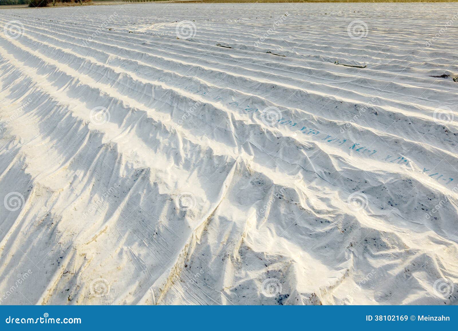
They use this spun woven stuff these days:
http://www.sciencephoto.com/image/26298/530wm/B6300272-Frost_protection-SPL.jpg
Oops, that last one is glass bells…wrong pic…I meant to show you this:
Interesting, I also learned a bit about what you are pointing out over the last several years from the two portable greenhouses which I have been using to keep my citrus trees alive through the winter in an area where they could not survive otherwise. It is surprising how effective they are at maintaining enough warmth for survival.
I keep large containers of water in each. I thought that they would aid in holding back the cold, and they appear to have done so. In the one unheated greenhouse the surface water only lightly froze once. That was when outside temps dropped down to the mid 20s F.
this is a good image
The optical window is 8-14u right in the peak of many earth based temps. Because it’s IR, even if the rest was blocked, it would shift to the window to cool.
Concrete needs a lot more time to cool, Grass, is just an air based insulator, top freezes, ground is still warm for a while.
The sky gets really cold. I had the telescope out a month ago, and it was in the low 40’s about 2:30am, but bitter, clear and calm. Heavy frost on truck, so I got the IR thermo out. Sky was -60F, 100F colder than air temp.A good part of the spectrum is 70 to over 100F colder than concrete temp, all day long. Part does get a lot of GHG spectrum, changes from 3.7W/m^-2 in about 1.8F making -40F, -38.2F(it changes depending the temp, I’ve done the calculations for -40F)Even if the whole rest of the spectrum was air temp, the window would still be quite cold, and conduction from those bands would warm things into the window where it would still cool to space.
Goldminor.
Try spraying some water in there…it will keep it much warmer.
If you have a well, the groundwater will be about the average yearly temp for your location. In Pasco county, that is about 72F.
Now, 72 degree water from overhead misters is very cold on a hot Summer day.
But on a cold night…it is steaming.
I kept most of an 80,000 sq ft shadehouse from ever getting below 50F by turning on the water.
I had the lace set up with drip irrigation, and for most of the plants that was all you ever needed.
But for flexibility, you also need to have overhead irrigation throughout, so you can put in plants that are too small and closely spaced for drip tubes, or occasionally other reasons. Plus i did a foliar feeding every week so that made it easy.
Instead of the rotating kind that throw water a long way in rather large drops, thus minimizing the number of sprinkler heads you need, i set up mist heads on every bay, spaced ten to twelve feet apart in one direction and ever five feet the other.
Then I had a series of zones valves and electromechanical timers connected to solenoid valves that rotated the flow of water into each bay for a few minutes every hour.
We only had two wells and only one was a large deep one. It could pump a few hundred GPM. So I could only turn on about 8 out of about 80 bays at one time.
But the steam (cold steam) spread the heat out evenly.
After about five minutes it was as warm as the water could make it, and the timers rotated the zone valves to the next zones.
So once you have the timers calibrated and synchronized, the water would just spray until it warmed up enough in the morning to turn it off.
For outside stuff, you sprayed with water in the morning to melt frost if it was above 32 (frost forms at 38)
and that was sufficient…the damage is done when the frost melts as the sun hits it…the melting frost takes latent heat from the leaves and burns them.
For temps below 32, you turn it on before it gets to freezing and leave it on until all the ice is melted the next day. Only once or twice did a freeze last into a daytime interval for more than a few hours.
So you have to know the temp everywhere…if it gets too cold and the water in the valves or lines begins to freeze before you open them…you are done for. Nothing you can do.
I knew a strawberry farmer who lost everything he had because him and his wife went to a movie one evening.
As soon as he walked outside and smelled the air, he knew his whole crop and every penny he had was gone. No way to unfreeze pipes and valves. If he could have got the water on, he would have had some damage perhaps, but he would not have lost much.
Anyway…turn some water on if you want it warmer.
Although…citrus takes four hours below 28F for any damage to occur, and cold, but with no damaging levels of cold, sweetens the fruit.
Back in those days, 1980s and 1990s, there was no internet. No twenty four hour weather stations, even if you had cable which rural Pasco did not have.
Weather info was spotty and hard to come by unless you paid for it. Some did, but even then most info was gleaned from observations made in real time on the spot.
There was a weather station with a weather fax machine on the roof of the USF College of Social and Behavioral Sciences building , but it was 30 miles away and was little use in the middle of the night anyway. They never did give me a key.
@ur momisugly Menicholas…Thanks for the added info. These are small greenhouses, 12’x7′. They tend to stay moist inside on their own. Perhaps that is why they hold back the freeze as you suggest “..Try spraying some water in there..”. I was happily surprised to note that they had that capability. There is a 30 gallon tub of water in each, and the only ice that developed a few times was no more than a 32nd”, whereas a bucket of water sitting outside had almost 2 inches of ice overnight.
“Another article stated that if the lower atmosphere warms, the upper atmosphere must cool, which makes no sense to me.”
It makes no sense to me either. Reading back posts of “Realclimate”, it looks like Gavin Schmidt was
“schooled” on this issue.
James B. Shearer says:
27 Feb 2005 at 6:51 PM
Eli, Gavin is arguing above that adding greenhouse gasses would cause the stratosphere to cool even if the stratosphere was not being warmed by the adsorption of UV and that this is the explanantion of stratosphere cooling. I am arguing that this is incorrect. If all warming was from below there would be no cooling.
Gavin, the gradient increases but the fixed point is the top of the atmosphere not the effective radiating level. As a result all layers warm with the amount of warming increasing as you move towards the surface. This means the effective radiating level rises.
Consider the top of the atmosphere as an arbitrarily thin gray body. Looking down from this layer we see the earth radiating at its black body temperature, TB. Looking up we see space at near absolute zero. So this layer will have temperature ((TB**4)+0**4)/2)**.25 or (.5**.25)*TB or .84*TB as claimed above. If the top layer is not arbitrarily thin but instead has emissivity e then its temperature will be TB*(2-e)**(-.25). In either case the temperature is independent of the details of the temperature structure below, the key point is that the total outgoing radiation must balance the incoming solar radiation.
[Response: Obviously radiaitve balance must be maintained, and I am not disputing that the effective radiative level will rise. Possibly, the solution to this is that in the real atmopshere the movement of this level is severely constrained (mainly by adiabatic cooling) and so cannot rise enough to produce your solution. I’ll think about this a little more…- gavin]
For more on simple “greenhouse” models and radiation levels, see
http://www-paoc.mit.edu/labweb/notes/Lecture_4.pdf
and/or
http://jennifermarohasy.com/2009/03/radical-new-hypothesis-on-the-effect-of-greenhouse-gases/
“
Leo Smith: Another effect of high altitude air traffic could be the soot produced by gas turbines depositing on clouds below, reducing their albedo.This theory was suggested by the late Professor D.K.Edwards who was a leading radiation heat transfer researcher. He also suggested that jet-setters bump along below 15,000 ft !
Soot depositing on clouds?
Hmmm…
What percentage of the Earth’s atmosphere receives solar radiation outside the Earth’s Shadow?
The Earth is about 8000 miles across, and about 90% of the atmosphere is below about ten miles…the 100 mb level.
So very nearly but actually very slightly more than half.
The Sun is much wider than the Earth, but also very far away. The limbs of the sun thus illuminate a little air above the portion of the surface that is unlit.
Plus, some of the light from the sun is bent inward towards the center of the Earths shadow.
This is why during even total lunar eclipses, the moon is still visible. Do you want to count that light and the air it passes through?
You might get an answer if you calculate the percentage of the time after sunset and before sunrise that constitute twilight as it relates to the entire nighttime period.
It is a lot of it, but it varies with latitude and season.
And then there are several types and definitions of twilight…civil, nautical, astronomical…
I al gonna stick with a little bit more than half.
Here is the shadow of the Earth, BTW, plainly visible during twilight. The grey part is the full shadow, the pink band is the Belt of Venus:
We have heard many times that there is not a good or detectable relationship between solar activity and global temperature. The proxy normally used is 10Be in soil.
Is there a good proxy for solar IR strength that is separate from both sunspots and 10Be?
If the upper atmosphere is very hot it surely radiates downwelling IR which is captured by water vapour and to a much lesser extent, CO2. That contributes to systemic warming. Creating O3 high in the atmosphere also contributes to warming. How does O3 warming compare with CO2 warming?
Prof Lu of Waterloo U holds that the O3 warming (or not) strongly affects the global temperature, particularly over Antarctica where the O3 fluctuation is large.
If the UV is not absorbed along the way down, it reaches the surface or the surface of a cloud. What then? How much is reflected back into space?
All things considered the combination of O3 creation and direct warming from the highly variable UV and EUV (100:1) points to a viable mechanism for producing significant changes in the temperature at ground level.
Charles You say “One recent article by NASA says that the Thermosphere (above 100,000 ft) has cooled in recent years due to decreased solar activity and a reduction in ultraviolet light. ”
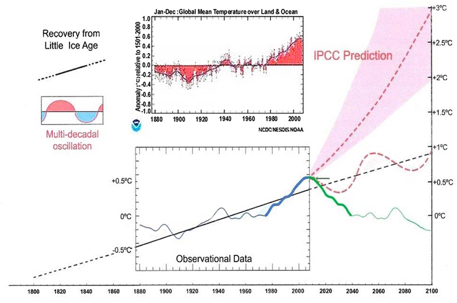
This fits very well with Figs 3,4,5 6,7,8,9,10 and 11 in my recent paper which says that the millennial temperature cycle peaked at about the end of the 20th century. Fig 11 provides a particularly obvious example.
Climate is controlled by natural cycles. Earth is just past the 2004+/- peak of a millennial cycle and the current cooling trend will likely continue until the next Little Ice Age minimum at about 2650.See the Energy and Environment paper at http://journals.sagepub.com/doi/full/10.1177/0958305X16686488
and an earlier accessible blog version at http://climatesense-norpag.blogspot.com/2017/02/the-coming-cooling-usefully-accurate_17.html
Here is the abstract for convenience :
“ABSTRACT
This paper argues that the methods used by the establishment climate science community are not fit for purpose and that a new forecasting paradigm should be adopted. Earth’s climate is the result of resonances and beats between various quasi-cyclic processes of varying wavelengths. It is not possible to forecast the future unless we have a good understanding of where the earth is in time in relation to the current phases of those different interacting natural quasi periodicities. Evidence is presented specifying the timing and amplitude of the natural 60+/- year and, more importantly, 1,000 year periodicities (observed emergent behaviors) that are so obvious in the temperature record. Data related to the solar climate driver is discussed and the solar cycle 22 low in the neutron count (high solar activity) in 1991 is identified as a solar activity millennial peak and correlated with the millennial peak -inversion point – in the RSS temperature trend in about 2004. The cyclic trends are projected forward and predict a probable general temperature decline in the coming decades and centuries. Estimates of the timing and amplitude of the coming cooling are made. If the real climate outcomes follow a trend which approaches the near term forecasts of this working hypothesis, the divergence between the IPCC forecasts and those projected by this paper will be so large by 2021 as to make the current, supposedly actionable, level of confidence in the IPCC forecasts untenable.”
.Fig 12 provides the cooling forecast out to 2100.
Fig. 12 compares the IPCC forecast with the Akasofu (31) forecast (red harmonic) and with the simple and most reasonable working hypothesis of this paper (green line) that the “Golden Spike” temperature peak at about 2004 is the most recent peak in the millennial cycle. Akasofu forecasts a further temperature increase to 2100 to be 0.5°C ± 0.2C, rather than 4.0 C +/- 2.0C predicted by the IPCC. but this interpretation ignores the Millennial inflexion point at 2004. Fig. 12 shows that the well documented 60-year temperature cycle coincidentally also peaks at about 2004.Looking at the shorter 60+/- year wavelength modulation of the millennial trend, the most straightforward hypothesis is that the cooling trends from 2004 forward will simply be a mirror image of the recent rising trends. This is illustrated by the green curve in Fig. 12, which shows cooling until 2038, slight warming to 2073 and then cooling to the end of the century, by which time almost all of the 20th century warming will have been reversed.
Norman,
As has been pointed out before here several times previously, the data since 2008, from which the forecast period on Fig. 12 runs, has already demonstrated both yours and Akasofu’s predictions to be wrong. The blue line has continued on a trajectory much more closely aligned to the IPCC forecast; in fact, a little on the high side of that as of end 2016.
“It’s just a flesh wound!”
(As you have pointed out before, you should know that it makes no difference)
See this Fig and a response posted on an earlier thread
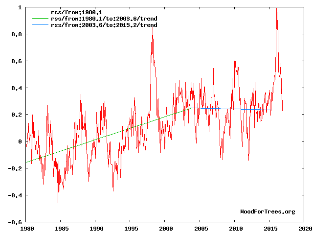
https://wattsupwiththat.com/2017/05/25/no-santer-et-al-have-not-refuted-scott-pruitt/#comment-2511654
and my reply
My main reason for showing the Akasofu curve was to show an example of an interpretation which at least honors the 60 year cycle which clearly exists over the last century. Here is my paper’s Fig 4 detailed interpretation as of end 2016 which shows the 2016 El Nino as the temporary deviation from the cooling trend which it most likely is.
The RSS cooling trend in Fig. 4 and the Hadcrut4gl cooling in Fig. 5 were truncated at 2015.3 and 2014.2, respectively, because it makes no sense to start or end the analysis of a time series in the middle of major ENSO events which create ephemeral deviations from the longer term trends. By the end of August 2016, the strong El Nino temperature anomaly had declined rapidly. The cooling trend is likely to be fully restored by the end of 2019.
Norman,
As Nick Stokes pointed out on the previous thread you linked to, global temperatures in 2009, 2010, 2011, 2012, 2013 and 2014, all of which occurred prior to the onset of the recent big El Nino, were all warmer than 2008, the supposed start of yours and Akasofu’s cooling trend.
Not only that, all of those years occurred during the weakest solar cycle in living memory and one of them, 2011, was also dominated by strong La Nina cooling conditions. What do you suggest was the reason for this, given that your prediction was for cooling and all normal climate forcings, apart perhaps from enhanced greenhouse forcing, were also indicating cooler conditions?
99% of the atmospheric mass is below 32 km. It’s these molecules that make conduction, convection, latent heat process possible, the processes that actually run the atmospheric heat engine. Above 32 km the lack of molecules mean radiation is the only mode of energy/heat movement. Without molecules, energy, heat, hot, cold terms and concepts fall apart.
Great point. Doesn’t that also mean that the high winds at upper altitudes require less energy to reach the same speeds than they would at a lower altitude?
In the end of the blog is a common mistake that the sun does not heat up the atmosphere. It does. The SW radiation absorbed by the surface is 167 W/m2 and the atmosphere absorbs 72 W/m2, together 239 W/m2. The main absorbing gas is surprise, surprise .. water 77 % and ozone 20 %. The LW radiation emitted by the Earth is absorbed by water 81 % and by CO2 13 %. And by the way, the absorption of CO2 happens below 1 km altitude.
Why is it so that sunshine (SW of it) is absorbed below 1km? If the WV curve so steep?
I referred to the absorption of LW radiation.
It seems likely that after the SO2 related affects of Pinatubo dissipated in the mid 90’s, there was some type of change that occurred in the Stratosphere, it cooled below the pre eruption temperature levels by almost 0.5 K and has been flat ever since.
http://data.remss.com/msu/graphics/tls/plots/sc_Rss_compare_TS_channel_tls_v03_3.png
Charles,
Nice write up…you may want to check your analysis software. The RAOB data looks fine.
I went to ruc.noaa.gov site & collected a years worth of Tuscon, Az for 2003 where your 00Z/12Z data was converged. Just looking at the tabulated data for 100mb, for example, shows temps varied quite a bit with extremes larger than your graph allowed. Below is 00Z Jan 1 to 12Z Jan 15.
LVL HGHT TMP DWPT WDIR WSPD
254 0 1 JAN 2003
4 100 30830 -52.7 -76.7 260 21
254 12 1 JAN 2003
4 100 30780 -52.5 -78.5 255 24
254 0 2 JAN 2003
4 100 30780 -51.9 -75.9 245 14
254 12 2 JAN 2003
4 100 ***** **** **** *** **
254 0 3 JAN 2003
4 100 ***** **** **** *** **
254 12 3 JAN 2003
4 100 ***** **** **** *** **
254 0 4 JAN 2003
4 100 ***** **** **** *** **
254 12 4 JAN 2003
4 100 30750 -52.7 -78.7 315 16
254 0 5 JAN 2003
4 100 30830 -47.5 -75.5 305 12
254 12 5 JAN 2003
4 100 30800 -48.7 -76.7 315 5
254 0 6 JAN 2003
4 100 30850 -48.1 -76.1 285 12
254 12 6 JAN 2003
4 100 ***** **** **** *** **
254 0 7 JAN 2003
4 100 30810 -47.5 -75.5 60 25
254 12 7 JAN 2003
4 100 ***** **** **** *** **
254 0 8 JAN 2003
4 100 30840 -49.7 -75.7 80 23
254 12 8 JAN 2003
4 100 ***** **** **** *** **
254 0 9 JAN 2003
4 100 30810 -49.1 -76.1 70 23
254 12 9 JAN 2003
4 100 30760 -49.1 -76.1 105 8
254 0 10 JAN 2003
4 100 30750 -46.5 -74.5 75 17
254 12 10 JAN 2003
4 100 30680 -50.1 -77.1 *** **
254 0 11 JAN 2003
4 100 30730 -46.1 -74.1 260 8
254 12 11 JAN 2003
4 100 ***** **** **** *** **
254 0 12 JAN 2003
4 100 ***** **** **** *** **
254 12 12 JAN 2003
4 100 30610 -51.7 -78.7 300 22
254 0 13 JAN 2003
4 100 30650 -50.1 -77.1 235 13
254 12 13 JAN 2003
4 100 30620 -50.5 -77.5 265 21
254 0 14 JAN 2003
4 100 30630 -51.3 -78.3 295 14
254 12 14 JAN 2003
4 100 30540 -51.1 -78.1 265 10
254 0 15 JAN 2003
4 100 30580 -49.7 -76.7 270 22
254 12 15 JAN 2003
4 100 30590 -51.9 -78.9 280 22
MIN TEMP -52.7
MAX TEMP -46.5
254 12 4 JAN 2003
4 100 30750 -52.7 -78.7 315 16
254 0 5 JAN 2003
4 100 30830 -47.5 -75.5 305 12
DIFF = 5.2
Same thing was seen at other times throughout the year and at different levels.
Jeff
https://en.m.wikipedia.org/wiki/List_of_large_volcanic_eruptions_of_the_20th_century
It seems that the increased volcanic activities in severity from the 1990s may have cause and effect for the temperature and CO2 ballance. When the Aerosol Gases and ash spread into and around the atmosphere by the jet streams as they raise. I don’t have access to the data for those gases or in the levels above what would effect the data in your article. I’m looking at the correlations of the volcanic activities and the over 18 year’s of stalled temperature increase and how your Arizona temperature/CO2 is nearer the Equator started converging and how long it took for the convergence in Alaska. Temperature decreases seem to trend after volcanic activities throughout our history and the CO2 ppm doesn’t seem to correspond to those changes. The larger the volcanic activities the more earth cools. And yet there seems to trend that the higher the CO2 the longer it takes to cool the lower levels.
*****CORRECTION*****
My previous post erroneously used 10mb data instead of 100mb. Below is the correct 100mb data from Tuscon, Az raob 00Z Jan 1, 2003 to 12Z Jan 15, 2003. Same effect is seen…just with colder temperatures.
254 0 1 JAN 2003
4 100 16320 -62.7 -81.7 270 57
254 12 1 JAN 2003
4 100 16280 -65.1 -83.1 32767 32767
254 0 2 JAN 2003
4 100 16310 -65.3 -82.3 305 43
254 12 2 JAN 2003
4 100 16360 -67.9 -85.9 305 46
254 0 3 JAN 2003
4 100 16390 -68.7 -85.7 295 30
254 12 3 JAN 2003
4 100 ***** **** **** *** **
254 0 4 JAN 2003
4 100 16380 -66.5 -83.5 270 33
254 12 4 JAN 2003
4 100 16320 -65.3 -82.3 300 37
254 0 5 JAN 2003
4 100 16340 -64.9 -83.9 305 39
254 12 5 JAN 2003
4 100 16330 -64.9 -82.9 295 26
254 0 6 JAN 2003
4 100 16340 -64.5 -82.5 340 28
254 12 6 JAN 2003
4 100 16340 -63.5 -85.5 335 37
254 0 7 JAN 2003
4 100 16360 -57.9 -82.9 340 21
254 12 7 JAN 2003
4 100 16390 -62.3 -85.3 0 26
254 0 8 JAN 2003
4 100 16420 -66.3 -86.3 335 21
254 12 8 JAN 2003
4 100 16450 -66.7 -86.7 310 16
254 0 9 JAN 2003
4 100 16470 -70.5 -89.5 310 16
254 12 9 JAN 2003
4 100 16470 -71.3 -90.3 240 10
254 0 10 JAN 2003
4 100 16400 -69.3 -89.3 235 62
254 12 10 JAN 2003
4 100 16370 -66.7 -88.7 245 44
254 0 11 JAN 2003
4 100 16350 -65.7 -86.7 265 49
254 12 11 JAN 2003
4 100 16340 -65.3 -85.3 280 40
254 0 12 JAN 2003
4 100 ***** **** **** *** **
254 12 12 JAN 2003
4 100 16430 -72.5 -91.5 32767 32767
254 0 13 JAN 2003
4 100 16450 -69.7 -90.7 280 45
254 12 13 JAN 2003
4 100 16460 -69.3 -88.3 290 41
254 0 14 JAN 2003
4 100 16450 -72.1 -91.1 285 48
254 12 14 JAN 2003
4 100 16450 -70.5 -90.5 270 52
254 0 15 JAN 2003
4 100 16400 -71.5 -89.5 260 73
254 12 15 JAN 2003
4 100 16390 -68.9 -82.9 32767 32767
MAX TEMP = -57.9
MIN TEMP = -72.5
254 12 6 JAN 2003
4 100 16340 -63.5 -85.5 335 37
254 0 7 JAN 2003
4 100 16360 -57.9 -82.9 340 21
LARGEST 12 HR SWING = 5.6
Not sure what you are saying JKrob. The Graph points for 2003 and other charts are year-long averages, only the two charts for 1995 and 1996 are daily values.
I haven’t read the comments thoroughly so apologies if this was mentioned, but my instinct for the difference in the years where the data converge is possibly due to instrumentation. I’m an electrical engineer and in a previous job helped develop balloon launched radiosondes and actually tested with NOAA. Is it possible that the make or model of the radiosonde has changed and that the stock of each location was used up at different rates? At the time they were using a Mark IV radiosonde (the manufacturer escapes me now). That implies that there was at some time a Mark III, II and I, right? Could the different models have different upper level temperature characteristics? In our testing I’ve seen that heat from the RF transmitter in the radiosonde can have an effect on upper air temperature measurements and in earlier models it may have skewed the data collection. Just a thought…
If by any chance aircraft were responsible, there would be no need to do anything since warming is beneficial .
We would know that we could always turn the knob down in the future when the temp was perfect.
What i see …. there is no convergence. There is a step change at 1996. There is no convergence before that, and there is no divergence after the lines magically come together. Makes me think there is a problem with this data.
I would think that the temperature of the atmosphere is directly related to a combination of heat source relative location and local extinction range of LWIR. At some point the extinction range becomes infinite and the radiation leaves the earth system. Secondarily atmospheric density is related to altitude and so to should be extinction range and with it absorbtion and re-radiation. Thirdly, as you go higher in elevation more of the horizon is exposed and less of the downward radiation is directed toward terrestrial objects not to mention the surface being beyond the extinction range of CO2 molecules, so less energy is available to (re)heat the surface.
I found the effect in the surface record in 1996 as well. It has a strong latitudinal component, I think it’s ocean cycles. N20-N30 the Temp in F response to 1 watt of clear sky day solar. These are from surface stations. and if you follow my name there’s a lot more graphs with regional looks at measured surface data.
Still waiting for Dr. Svalgaard to show up and tell us all, um…all the stuff we got wrong…?
If radiative gases cool the earth by radiating heat to space, what is the effect of increasing the concentration of radiative gas?
Just asking.
I have asked the same question. The adiabatic theory on CO2 is that it acts as a coolant, just like water vapor ……. absorbs heat, rises, releases heat at top of atmosphere.
The equilibrium temperature of a radiantly heated object is a function of the correlation of its absorptivity=emissivity spectrum with its source and sink spectra , eg the spectrum of the earth as seen from space and the power spectrum of the 5.5-e6 of the celestial sphere covered by the Sun’s disk and the rest at so near 0 it macht nichts . See http://cosy.com/Science/warm.htm#EqTempEq .
The change in our spectrum as seen from outside due to additional CO2 at these levels is de minimis .
And no spectral effect can explain why the bottoms of atmospheres are hotter than that calculated on the basis of the spectrum as seen from outside .
Interesting observations. I have a problem with this: The sun is the main driving force for changes in temperature at high altitudes, less so for high latitude locations.
For high latitudes the sun travels more of the atmosphere, than at lower latitudes, where it just passes through. Just a thought.
The upper atmosphere is poorely known and the up-down mechanisms as well.
In fact, many research have pointed out that the upper atmosphere, (Stratophere, Mesosphere, Thermosphere), is cooling since the late 70s/beginning of the 80s (Same time as the ENSO shift). In those times, the sun’s activity was not so low as it is currently, altought it has been proven that the sun’s activity has a tremendous effect on thermospheric temperatures and more relatively one the mesosphere/stratosphere.
So what is the cause of that cooling ? The sun has surely a role in the last decade but prior to that ?
The only interesting theory that i found is that this cooling could have been produced by the ENSO shift, changes of wind patterns and gravity waves. Here is the study :
http://onlinelibrary.wiley.com/doi/10.1002/jgra.50370/pdf
And 2 quotes :
“Manabe and Wetherald [1967] first showed that an increase in CO2 content in the atmosphere would heat the atmosphere below about the tropopause (by absorbing IR radiations from the ground) and cool the atmosphere above that level (by radiating thermal energy to space). Roble and Dickinson [1989] calculated the degree of cooling above 60 km altitude that one would expect for a doubling of greenhouse gas content at that altitude. They estimated a global mean cooling of 50 K near 350 km altitude. Holt and Zhang [2008], however, in considering the 1978–2007 database of incoherent scatter radar measurements of ion temperature collected at 375 km above Millstone Hill (43 ı N, 289 ı E), found a noontime cooling rate of 47 K per decade, or a 141 K decline over the span of their measurements. As the CO2 concentration increased only 12% during this time period, the simulation would estimate only an 6 K decline. Donaldson et al. [2010] conducted an independent analysis of the 1966–1987 Saint Santin (45 ı N, 2 ı E) radar database and confirmed the Holt and Zhang [2008] finding. In light of this stark factor-of-20 disagreement between theory and observation, processes other than CO2 cooling have been sought to explain the observations. Based on the Saint Santin data, Walsh and Oliver [2011] suggested some agency of O3 as the cooling source, based on the coincidence in time between the beginning of the temperature decline and the beginning of a strong decrease in O 3 content in the lower atmosphere. Laštovicka [2012] noted, however, that the longer 1978–2007 Millstone Hill data showed that the
temperature continued to decline beyond 1994, when the O3 content began a long recovery. [ 3 ] During our efforts to identify the cause of the great temperature decline in the thermosphere, we have noticed a correlation between the behavior of that temperature and the behavior of ENSO (El Niño–Southern Oscillation) activity, both in the timing of an onset of change, a subsequent linear trend, and decadal variations about that trend. This recognition has led us to ask if gravity waves, produced by wind action over the oceans and propagated to the upper atmosphere, may be responsible for cooling that upper region. Recent simulations [e.g., Yigit and Medvedev, 2009] show that gravity waves are expected to cool the thermosphere on the order of 100 K, the order of long-term cooling observed. We know of no other agency capable of cooling the thermosphere by that amount long term.”
“Why is the cooling so much larger than expected, (2) why has the cooling lasted so long, and (3) why is the thermospheric density response to the cooling so small? We have speculated that gravity waves may have caused this cooling, based on recent simulations that show that gravity waves are expected to cool the upper thermosphere by an amount comparable to the long-term cooling observed. A gravity wave proxy formed from the nontidal fluctuations in T° ion showed a positive long-term trend throughout its timeline, consistent with the increasing cooling observed. Fluctuations of T° ion about its long-term trendline were seen to anticorrelate both with fluctuations in the gravity wave proxy and with decadal fluctuations in El Niño–Southern Oscillation (ENSO) activity. The time scales of the long-term trend and the decadal fluctuations are characteristic of the ocean, not the atmosphere. We have suggested that the following scenario may explain these behaviors: (a) the climate regime shift of 1976–1977 launched slow Rossby waves across the oceans, waves which continue to propagate to this day; (b) winds over this increasingly corrugated ocean have launched increasing fluxes of gravity waves into the atmosphere; (c) these increasing fluxes of gravity waves have propagated to the thermosphere to produce increasing amounts of cooling; and (d) the decadal increases in winds associated with the decadal increases in ENSO activity have produced decadal increases in gravity wave fluxes, which, in turn, have caused decadal cooling in the thermosphere. The strong thermospheric cooling seen would be expected to produce thermospheric density declines much larger than those observed via satellite drag if the density at the base of the thermosphere were unchanging. We have noted that a lowering of the turbopause by about 4 km would raise atomic oxygen densities and completely compensate for that large expected density decline at 350 km altitude and referenced evidence of that lowering. We have asked if the heat pumped by gravity waves from the upper thermosphere to the lower thermosphere may augment the positive temperature gradient in the turbopause region, thereby making it more stable against the development of turbulence, and hence lowering the turbopause itself. Our proposed answers to our three posed questions are that the magnitude of the cooling is due to the agency of atmospheric gravity waves, that the length of the cooling is due to agency of ocean Rossby waves, and that the small density response is due to the lowering of the turbopause.
The ocean effect is a long-term transient response to forcing of unknown origin. The atmospheric effect is a steady state response to ocean forcing. This scenario may have validity, but it is unproved. The ocean Rossby wave source is purely speculative. Those Rossby waves, if they should exist, cannot be detected amongst the larger ocean eddies with current observational capabilities. (We ask if the very smallness of these ocean waves may be essential in that it leads to atmospheric gravity waves that are able to propagate to the upper thermosphere without growing to their breaking amplitude and dissipating at lower altitude.) For the existence of increasing amounts of gravity waves in the thermosphere, however, we have the evidence from our data of the increasing amounts of nontidal fluctuations in temperature. If the theorists and modelers [e.g., Walterscheid, 1981; Yi ̆git and Medvedev, 2009] are correct, this increasing gravity wave flux should increasingly cool the thermosphere. 42 ] These speculations need broad vetting by additional studies based on other data sets and of applicable theory. [ 43 ] We believe that the magnitude of the thermospheric temperature decline has been so great that the CO2 theory of its cooling cannot be maintained. It is certainly possible, however, that increased greenhouse warming at surface level has initiated the train of events that has led to the cooling by others means.”
Oliver, W. L., S.-R. Zhang, and L. P. Goncharenko (2013), Is thermospheric global cooling caused by gravity waves?
A similar question relating to temperatures at different altitudes has been investigated in tge southern hemisphere by Erl happ. Focuses on observations not models. https://reality348.wordpress.com. Chapter 6 highlights temperature divergence in winter but none in summer, despite decades passing. So Well mixed CO2 cannot choose when to emit IR but highly variable ozone might if the polar vortex lowers the tropopause closer to ground level.
Well, I can see this was a nice waste of time. Find errors in the analysis & it is completely ignored.
Peer Review via blogs…yeah, right.
Jeff, i only check this site occasionally. I did reply to your post earlier. Sorry about that.
Follow up: Many people’s belief that the change in temperature was probably caused by instrument changes. This was a valid criticism. Here is a link to a rather exhaustive study of various radiosonde instruments in 2010.
https://www.wmo.int/pages/prog/www/IMOP/publications/IOM-107_Yangjiang.pdf
Greg posted “Well if it starts at the surface, why is it called UPPER atmosphere? Who defines it in that way apart from the author?”
I have worked in weather related activities for almost 70 years and 36 of those at what was, and is, called Upper Air Stations, even though they are on the ground.
One fellow criticized me for the statement: “Another article stated that if the lower atmosphere warms, the upper atmosphere must cool, which makes no sense to me.” My problem with that was the MUST part of the statement.
Here is a direct quote: Jeffrey Masters, Ph.D. — Director of Meteorology, Weather Underground, Inc. “Climate models predict that if greenhouse gases are to blame for heating at the surface, compensating cooling must occur in the upper atmosphere. We need only look as far as our sister planet, Venus, to see the truth of this theory. Venus’s atmosphere is 96.5% carbon dioxide, which has triggered a run-away greenhouse effect of truly hellish proportions. “
I did this little study because I was interested in the results, I don’t get paid, I have no grants, just me.
Since this is a follow up, I added three more stations to the list of stations where the diurnal temperatures aloft have converged. San Diego, California in 2010, Dodge City, Kansas in 2009, and Brownsville, Texas, also in 2009.
The surface temperature of Venus , 2.25 times that of a gray body in its orbit is absurdly greater than anything which can be explained by spectra .
Anyone who claims that it can be , show us the quantitative equations and their experimental validation . It’s been decades now and such foundational testable physics has never been presented .