From NASA Goddard via the OCO-2 Satellite
Carbon dioxide is the most important greenhouse gas released to the atmosphere through human activities. It is also influenced by natural exchange with the land and ocean. This visualization provides a high-resolution, three-dimensional view of global atmospheric carbon dioxide concentrations from September 1, 2014 to August 31, 2015. The visualization was created using output from the GEOS modeling system, developed and maintained by scientists at NASA. The height of Earth’s atmosphere and topography have been vertically exaggerated and appear approximately 400 times higher than normal to show the complexity of the atmospheric flow. Measurements of carbon dioxide from NASA’s second Orbiting Carbon Observatory (OCO-2) spacecraft are incorporated into the model every 6 hours to update, or “correct,” the model results, called data assimilation.
As the visualization shows, carbon dioxide in the atmosphere can be mixed and transported by winds in the blink of an eye. For several decades, scientists have measured carbon dioxide at remote surface locations and occasionally from aircraft. The OCO-2 mission represents an important advance in the ability to observe atmospheric carbon dioxide. OCO-2 collects high-precision, total column measurements of carbon dioxide (from the sensor to Earth’s surface) during daylight conditions. While surface, aircraft, and satellite observations all provide valuable information about carbon dioxide, these measurements do not tell us the amount of carbon dioxide at specific heights throughout the atmosphere or how it is moving across countries and continents. Numerical modeling and data assimilation capabilities allow scientists to combine different types of measurements (e.g., carbon dioxide and wind measurements) from various sources (e.g., satellites, aircraft, and ground-based observation sites) to study how carbon dioxide behaves in the atmosphere and how mountains and weather patterns influence the flow of atmospheric carbon dioxide. Scientists can also use model results to understand and predict where carbon dioxide is being emitted and removed from the atmosphere and how much is from natural processes and human activities.
Carbon dioxide variations are largely controlled by fossil fuel emissions and seasonal fluxes of carbon between the atmosphere and land biosphere.
For example, dark red and orange shades represent regions where carbon dioxide concentrations are enhanced by carbon sources. During Northern Hemisphere fall and winter, when trees and plants begin to lose their leaves and decay, carbon dioxide is released in the atmosphere, mixing with emissions from human sources. This, combined with fewer trees and plants removing carbon dioxide from the atmosphere, allows concentrations to climb all winter, reaching a peak by early spring. During Northern Hemisphere spring and summer months, plants absorb a substantial amount of carbon dioxide through photosynthesis, thus removing it from the atmosphere and change the color to blue (low carbon dioxide concentrations). This three-dimensional view also shows the impact of fires in South America and Africa, which occur with a regular seasonal cycle. Carbon dioxide from fires can be transported over large distances, but the path is strongly influenced by large mountain ranges like the Andes. Near the top of the atmosphere, the blue color indicates air that last touched the Earth more than a year before. In this part of the atmosphere, called the stratosphere, carbon dioxide concentrations are lower because they haven’t been influenced by recent increases in emissions.
Joseph Fournier writes on Facebook of the surprising thing he’s found:
I have quantified the average ‘lag’ between the seasonally detrended monthly rate of CO2 concentration change at both the South Pole and at Mauna Loa and there is virtually ZERO LAG as indicated by the symmetric function around the y-axis. The second curve is the ‘lag’ in the number of months between when the Pacific Trade Winds decelerate and when the seasonally detrended monthly rate of change in the tropospheric CO2 concentration as measured at the South Pole station reaches its maximum growth rate. This model ignores empirical data as it shows that all the CO2 emissions are in the North Hemisphere and yet monitoring stations in both hemispheres suggest a common area source in the tropics.

dobre próbowanie ,lubię kiszone ogórki, co to zmieni ,nie czytajcie danych z NOAA I NASA . Jestem Copernikus Mazowia i nie znoszę ruskie buty.
We have 500 days to a void climatic chaos. 2 years ego .. 😉
A “greenhouse effect” as in laboratory observations extrapolated to global proportions through inference and models (i.e. hypotheses) that have demonstrated low skill to represent let alone prophecy past and future states.
The problem is that the CO2 GHG effect on Temp lapse rate cannot be replicated in a lab setting.
The atmosphere T lapse rate is a gravitometric emergent property of compression of a air, and the reverse lowering of pressure (and thus mass) as one measures T vertically in a column of air parcel from the surface to the stratosphere. The T lapse rate is adiabatic in that no additional energy (heat) is added, yet T decreases because pressure (and thus mass) decrease. Most fundamentally, this is both a manifestation of Energy Conservation (1st Law) and net heat flow is always hotter to colder (2nd Law). No lab set up can simulate/replicate 20 km of vertical column air.
Earth’s Forest Area 9 Percent Greater Than Thought
Satellite survey finds hidden forests all over the world.
http://reason.com/blog/2017/05/12/earths-forest-area-9-percent-greater-tha
The extent of forest in dryland biomes
Abstract
Dryland biomes cover two-fifths of Earth’s land surface, but their forest area is poorly known. Here, we report an estimate of global forest extent in dryland biomes, based on analyzing more than 210,000 0.5-hectare sample plots through a photo-interpretation approach using large databases of satellite imagery at (i) very high spatial resolution and (ii) very high temporal resolution, which are available through the Google Earth platform. We show that in 2015, 1327 million hectares of drylands had more than 10% tree-cover, and 1079 million hectares comprised forest. Our estimate is 40 to 47% higher than previous estimates, corresponding to 467 million hectares of forest that have never been reported before. This increases current estimates of global forest cover by at least 9%.
http://science.sciencemag.org/content/356/6338/635
So should we believe the NASA CO2 models, given that they are entirely based on satellite data? Or should we consider the level of uncertainty that is fundamentally inherent in satellite based sensors, and the potential range of error that these could have on the physical characteristic that they are measuring?
But how would the NASA video display error bars on their pretty graphic? Perhaps they could overlay the graphic with an orbital chart showing the path of the satellite, and only display those parts of the earth that they actually have collected data from?
And I do wonder how a satellite can determine the changing concentration of CO2 with height? Does that mean slant measurements are also collected, and integrated over multiple passes? So then they would be effectively calculating average concentrations over time, which would also make for a boring 3D representation.
I’m guessing that, if NASA blocked out all the model-based data and only showed the satellite based data, there might not be much left to show on their graphic.
You are clueless
Here is the level one ATBD
http://disc.sci.gsfc.nasa.gov/OCO-2/documentation/oco-2-v7/OCO2_L1B%20ATBD.V7.pdf
This is level 2
https://co2.jpl.nasa.gov/static/docs/OCO-2%20ATBD_140530%20with%20ASD.pdf
Pauly,
One of the problems with the OCO-2 data is that it is spotty. Low level clouds interfere with getting readings. Thus, when you look at one of their raw data maps, you frequently see individual spots in the oceans. They have to do a lot of interpolating or averaging over time to get complete coverage.
For once, I agree with Mosh.
The press release said that the animation was for the period of September 1, 2014 to August 31, 2015. However, what was shown is only for March to July 2015. The animation looks different from others I have seen in that previously they showed low CO2 in the NH in the Winter, with a sudden release in the early Spring as things start to warm up and bacteria become active decomposing the leaf litter. Then, with trees leafing out in May, there is a dramatic drop in CO2 through the Summer. I also don’t see the strong oceanic sources in the Tropics, nor the Amazon Basin that were previously shown. I hope that this is a result of the color scheme chosen rather than NASA corrupting the data for a storybook.
Seems awfully convenient, dudn’t it? Kind of nags at you… What’s that phrase? Something by omission.
Ooo, ooo – I know what the “something” by omission is! I will just say, it is quite dishonest whether in court or in science, when one does not tell the truth, the whole truth, and nothing but the truth.
Great assist, Not Chicken Little! 🙂
Wouldn’t younexpect zero lag in seasonally adjusted data?
Am I missing something here?
daleko między nami pomiędzy rosyjskim szczęściem jest miejsce dla nieba
[Far between us is a place for heaven between Russian happiness…
The mods would point out that few Poles are happy being between Russia. And anywhere else. .mod]
Strange that those noxious clouds of CO2 can’t make it south of the equator even tho’ their half life in the atmosphere is thousands of years.
There’s plenty of CO2 below the equator… and CO2 isn’t toxic to humans at 400 ppm. So it’s not strange at all……
P.S.: The fact that the NH concentration of CO2
is greater than the SH concentration of CO2 is very good
evidence that the additional CO2 in the atmosphere is due to man.
And it’s also good evidence that the CO2 is absorbed / consumed, mostly by plant life, just about as fast as it is created, partly by humans.
Greater land mass in the NH than in the SH. Evidence it’s Land and not Man?
Plus the video’s “seasonal” only covers the months when it is cool to warmer for the NH and cool to colder for the SH.
Evidence of Man’s influence on the message? Perhaps.
crackers345,
It isn’t a full year of data!
You are Crackers.
crackers345, you claim that the shift in the isotopic ratio implicates anthropogenic fossil fuel burning. You left a URL that leads to “realclimate” – with this nugget:
Fossil fuel is more negative in δ13C than the atmosphere. Keeling 2011: “Atmospheric δ13C has decreased by ∼2 ‰, from -6.4 ‰ in 1850 (Suess, 1955; Friedli et al., 1986) to -8.4 ‰ in 2012 (Keeling et al., 2005 …”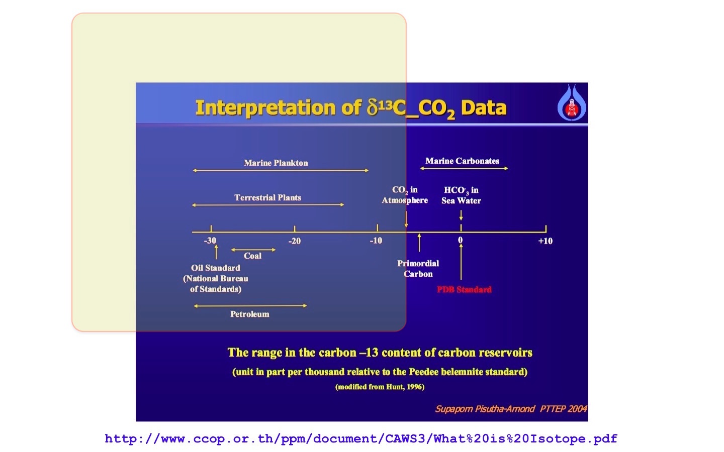 Terrestrial plants, and marine plankton are prime examples.
So, in the modern atmosphere, CO2 has a δ13C of about -8‰. Coal has a δ13C of about -23‰ to -28‰ Oil tends to be even further negative, -25‰ to maybe -33‰ …
But, there are many other sources that are even further in the negative region of δ13C. The isotopic shift mentioned by Keeling 2011 (above) simply means that a carbon source, with a more negative value of δ13C than the present CO2, is finding its way into the atmosphere.
So, any carbon source that vents to the atmosphere with a more negative value than about -9‰ would slew the present atmospheric δ13C to a more negative value … certainly, fossil fuel burning, will do that … but
Lee 2016 tells us: ”… biogenic δ13C values from soil CO2 studies along transform plate boundaries elsewhere, such as the San Andreas fault (−21.6 to −23.7 ; ref. 14).” The dilution of atmospheric CO2 with soil CO2 (as noted) will mimic Mannkind’s burning of fossil fuels.
Pisutha-Amond 2004 has a nice chart:
Jones & Grey 2011: ”An important characteristic of biogenic methane produced in sediments …, it is remarkably 13C-depleted (δ13C typically around -60 to -80‰; Whiticar, Faber & Schoell, 1986; Jedrysek, 2005; Conrad et al., 2007) compared with either allochthonous terrestrial plant detritus (δ13C value from C3 plants around -27‰; Peterson & Fry, 1987) or phytoplankton (δ13C typically around -25 to -35‰; Vuorio, Meili & Sarvala, 2006). Isotopic fractionation during utilisation of methane by MOB can lead to further 13C-depletion (by up to 20‰; Summons, Jahnke & Roksandic, 1994; Templeton et al., 2006).… strikingly low δ13C …”
Whiticar, Faber, & Schoell 1986: “Methane in marine sediments can be defined isotopically by δ13C −110 to −600‰, … In contrast, methane from freshwater sediments ranges from δ13C −65 to −500‰. …”
The dilution of atmospheric CO2 with oxidized biogenic methane, as noted, will mimic Mannkind’s burning of fossil fuels.
Brian, how about stating your argument and conclusion before
providing a bunch of quotes and links? I have no
idea what you’re trying
to say.
Clyde: the data
go way back.
Earth is not a greenhouse, CO2 is not the problem. Let’s look at who started and propagates this myth…
The UN & opportunistic, sympathetic governments like the USA who hope to cash in with taxes, fees and fascist policies to punish their population. The degree of covalent government involvement with globalist driven climate change in the USA makes me fighting mad!!!!
“The degree of covalent government involvement with globalist driven climate change in the USA makes me fighting mad!!!!”
Good! A *lot* of us feel the same way. We are in the process of straightening our government out on this issue. It’s taken a long time, but the tide seems to be turning.
And the temperatures are not climbing even with the extra CO2 in the atmosphere. Dishonest people may be able to manipulate the temperature charts to show warming, but they can’t manipulate a person’s personal thermometer. Reality will eventually set in.
This whole project by NASA using satellites and complex display graphics to identify sources, sinks and variations in CO2 was and is a colossal waste of tax payers money. Dig deeper into the science and discover that CO2 does not now, has never had and will never have a significant effect on climate.
Here is why:
1) Essentially all absorbed outgoing longwave radiation (OLR) energy is thermalized.
2) Thermalized energy carries no identity of the molecule that absorbed it.
3) Emission from a gas is quantized and depends on the energy of individual molecules.
4) This energy is determined probabilistically according to the Maxwell-Boltzmann distribution.
5) The Maxwell-Boltzmann distribution favors lower energy (longer wavelength) photons.
6) Water vapor exhibits many (170+) of these longer wavelength bands.
7) The Maxwell-Boltzmann energy distribution in atmospheric gas molecules effectively shifts the OLR energy absorbed by CO2 molecules to the lower energy absorb/emit bands of water vapor. The ‘notches’ in top-of-atmosphere measurements over temperate zones demonstrate the validity of this assessment.
8) As altitude increases (to about 10 km) the temperature declines, magnifying the effect.
@ur momisugly Dan Pangburn
May 12, 2017 at 7:30 pm: Yes Dan, that is what real physics/icists know, along with the real role of water vapour, latent heat transport, the instantaneous expansion and buoyancy uplift from thermalisation. This will not go away, no matter what. Thanks.
That visualization clearly showed CO2 changes were seasonal, and then the narrator only asserted something assumed but not seen in the data, that is, mankind’s contributions to CO2 flux.
The CO2 flux in that data viz is completely swamped by natural fluxes.
The text of that presser stated, “It [CO2] is also influenced by natural exchange with the land and ocean.”
They can’t admit the global CO2 flux is vastly dominated by natural exchange.
OCO-2 was designed to detect and measure anthropogenic CO2 sources, based on what is stated in the technical design statements on their own site. In fact the data analysis show that those anthropogenic sources are NOT visible above the natural CO2 background, no matter how the data are massaged or visualized. The OCO-2 analysis confirms what biogeochemical carbon cycle biologists have always known, that humans do not have a detectable influence in the global carbon cycle. CO2 never accumulates in the atmosphere, it is constantly being scrubbed out into the vast subsurface pools at the rate shown in the 1964 atomic bomb 14CO2 curve. Even if human CO2 flux is now 4 percent of natural CO2, then the amount of CO2 in the atmosphere today is 4 percent of 400 ppm or 16 ppm.
Human CO2 is rapidly mixed in the atmosphere, and rapidly mixed into the natural CO2 sinks. Most of the increase in CO2 since 1850 is due to the natural flux increases that began with the exit from the little ice age, from biotic and abiotic (ocean) factors.
No.
OCO (the original which failed to achieve orbit) and OCO-2 were never inteneded to to just measure A-CO2.
OCO-2 is 3 spectrophotometers. 2 measure CO2-adsorption of wavelengths of the reflected sunlight, and 1 spectrophotometer is measuring an O2 relevant adsorption wavelength for relative comparison of CO2 adsorption bands.
Thus the OCO-2 sensors only measure CO2. There is no ability to discriminate natural CO2 adsorption from anthropogenic CO2 adsorption. To believe differently from that is to think that the measured O-C-O molecule “padsorption reading is that the column molecules “know” how to differentially adsorb IR radiation depending on whether they were predominately from a coal molecule reacting with O2 or a decayed leaf carbon reacting with O2.
joelobryan,
You said, “OCO (the original which failed to achieve orbit) and OCO-2 were never inteneded to to just measure A-CO2.”
While it isn’t possible to separate Anthro-CO2 from natural in the maps , I believe the original hope was to be able to identify anomalously high CO2 levels in the vicinity of major coal burning power plants and urban areas with high per capita consumption of fossil fuels. Thus, they could say, “See, we told you that Man was responsible for the increase in CO2.” Unfortunately (for the alarmists), it isn’t evident that Anthropogenic sources dominate, even in the NH. Anthro-CO2 isn’t even obvious in the US during the Winter, when plants and bacteria are dormant but humans are using even more fossil fuels to heat their homes. In examining past-published OCO-2 maps, I could see an area in China that appeared to be anomalous. The Amazon Basin looked unusual, and was perhaps a result of land clearing and burning. There were some unusual ‘hot spots’ in Indonesia that were more difficult to attribute to a particular source, but it again was probably forest clearing. The bottom line, from my inspection, is that natural sources dominate the production and sequestration of CO2 with very few exceptions. Thus, one cannot unequivocally state that the excess CO2 is anthropogenic because the other processes would continue in the absence of Man, and if some other process besides ‘greenhouse gases” was responsible for increasing temperatures then there would be increased oceanic outgassing, and that would lead to increased vegetation which in turn would create more CO2 when it dies and decays.
The OCO was designed with the intention to have the ability to resolve “regional” surface sources of CO2 from any source.
The underlying intention was to resolve anthropogenic sources from “natural” regional areal sources over a couple years with ground based calibration of the satellite spectrometers since the methodology of the satellites only worked from the boundry layer to about 10k altitude where the aircraft measured CO2.
I did not say, or intend to claim, that the OCO was designed to “only” measure anthropogenic CO2.
I’ve read some of the science mission statements and one of the underlying papers for the design of the OCO. My interpretation of the intent of the people who created the OCO was that they wanted to map the anthropogenic CO2 sources with the intention of confirming their pro-global warming political bias. It’s sad to see the obvious global warmist bias in NASA and JPL web pages for a “science” mission.
The current “analysis” and presentation of data also clearly show a warmist bias, they are trying to show something that is not in the data. It is obvious to anyone that looks at the graphics that anthropogenic sources of CO2 can NOT be resolved from natural sources. They underestimated the amount of smearing of 4 percent in the boundry layer. The OCO-2 could never look into the boundry layer in the first place.
BTW, I agree with Clyde’s response. The OCO-2 worked fine, it found exactly what most any biologist or biogeochemical cycle ecologist would expect for a global view of CO2 sources and sinks. If someone wants to fly the same spectrometers 1000 meters over a coal power plant, they could see the CO2 coming out of the smokestacks, but that’s not a global picture.
I’ve watched the clip a few times now including at YouTube’s 0.25 speed . I can’t see any indication that high concentrations are coming from the industrialized urban areas one AlGoreWarming blames . Indeed much seems to be billowing from biologically lush areas like equatorial Africa .
I will be getting to https://www.esrl.noaa.gov/gmd/annualconference/ in Boulder the 23rd & 24th . Their website is partially down for some maintenance this weekend , but I see from my notes from 2015 , I met David Crisp , one of the main guys in the OCO-2 project . I see he’s got a YouTube : href=” https://www.youtube.com/watch?v=JYyhMQzcVlY” > David Crisp: Measuring atmospheric CO2 from space – 24 April 2015 .
Struck me as a bright guy , one of the few who knows APL . I do hope he will be there again this year . Look forward to a much more extensive conversation .
Somehow I got that anchor syntax wrong . Worth highlighting the vid anyway .
Odd that it doesn’t have the world’s constant CO2 hot spot: Hawaii. Vulcanism. Every day.
I just watched the video. Maybe somebody already brought this up but, the title of the video says “seasonal changes” yet it only covers March 1, 2015 to July 31, 2015.
That’s about early spring to mid-summer. Hardly “seasonal” for either hemisphere.
So what happened when human emissions leveled off, as reported recently over, what is it, 2 years? No change in the Hawai’i measurements? No, it cannot be that they got it wrong. Perhaps they are still celebrating the lifting of guilt. Please share with us, beloved warmistas. Not that any of their gas budgets are worth a Tinkers Curse, bur all the same, we would like to know…..
OCO2 was a riposte to JAXA, which made Nasa-GISS look silly. Did not work out too well, so currently all is smoke and mirrors (with credit to Rud).
Brett,
With constant CO2 emissions, CO2 still would go up in the atmosphere, but as the CO2 pressure goes up, the sinks (oceans and vegetation) will absorb more CO2, thus the increase rate will go down. That will end when emissions and sinks are equal, that is at around 500 ppmv for the current emissions.
Why is the angle in the video chosen so that one cannot see the Northern hemisphere, or the location of CO2 on the map, instead of choosing a vertical look?
“During Northern Hemisphere fall and winter, when trees and plants begin to lose their leaves and decay, carbon dioxide is released in the atmosphere, mixing with emissions from human sources. This, combined with fewer trees and plants removing carbon dioxide from the atmosphere, allows concentrations to climb all winter, reaching a peak by early spring. During Northern Hemisphere spring and summer months, plants absorb a substantial amount of carbon dioxide through photosynthesis, thus removing it from the atmosphere and change the color to blue (low carbon dioxide concentrations).” == From this it is clear that during high CO2 regime in the atmosphere the energy availability to convert in to temperature through greenhouse effect is practically very low; and during low CO2 regime in the atmosphere though the energy availability to convert in to temperature through greenhouse effect is high the temperature rise will be low with low CO2. This clearly demonstrate that the global warming is insignificant with CO2 raise from fossil fuel burning.
Dr. S. Jeevananda Reddy
Previous animated maps from OCO-2 have shown that bacterial oxidation essentially shuts down during the cold Winter, except maybe in the southern US and in similar latitudes in Europe and Asia. When I have previously examined the OCO-2 maps I looked carefully to try to find elevated CO2 from places like the Four Corners power plants and urban areas heating buildings. I didn’t see it. It makes me wonder why it is now being claimed to be there.
They use the time honored technique of “Hand-wavium” to find anthropogenic CO2 source signals in OCO-2 data.
Same here, the basic data is being “massaged” to show only what they want to see. Read some of the statements of the mission scientists that created the OCO missions, clearly biased. The null hypothesis prevails, there is no significant anthropogenic source of CO2 in the global biogeochemical carbon cycle.
It looks to me that the “natural” sources and sinks were grossly underestimated. Certainly in the tropics.
bw,
Yes, I suspect that the researchers were surprised at the amount of outgassing from the tropical oceans and the rapid pull-down of biogenic CO2 by trees leafing out in mid-latitudes. But, that was the whole point of the OCO missions — to learn more about the carbon cycle. Now, if they would only learn from their experience and not try to put a spin on the data!
Dr. Reddy,
Average CO2 release by humans is 0.01 ppmv/day. Even if concentrated in about 10% of the earth’s surface and the ability of the satellite to focus on specific spots during a longer period, it will be a hell of a job to find the extra CO2 from human emissions.
Still there are other problems with the data, as in previous published monthly data, high levels of CO2 where found over the N.E. Atlantic, where on of the largest CO2 sinks is situated…
Actually, it’s about 16 ppm per day, or year, or at any time since the continuous flux rate reached 4 percent of the total CO2 flux. In the early 20th century anthropogenic CO2 flux was about 1 percent of the total. After several decades, the atmosphere reached approximate equilibrium at about 1 percent total CO2.
As the anthropogenic flux gradually increased to 2 percent of the total flux, the total CO2 mass in the atmosphere approached .02 times say 300 ppm, or 6 ppm of the total. By 1958 the flux was maybe 3 percent of the total, or was .03 times 315 which is nearly 10 ppm. Now that the third world is cranking out coal fired power plants, the amount in the atmosphere will approach 16 ppm, at the atmosphere equilibrates. Just as a river will equilibrate at a new level when you add 4 percent to the flow rate.
bw,
You are mixing a lot of things together which don’t make any sense…
Human emissions reach about 9 GtC/year nowadays or ~4.5 ppmv/year or 0.0123 ppmv/day worldwide.
Even if concentrated in 10% of the world’s total area, that still is only some 0.1 ppmv/day. Or about the resolution of the OCO-2 satellite.
The satellite only measures midst of the day, thus depending of (lack of) wind speed the 0.1 ppmv/day still may hang around or blown away into the bulk of the atmosphere. Even if they use the possibility to focus on specific spots to enhance the resolution, it will not be easy to trace the human contribution.
For the rest, the satellite can’t make a distiction between the origins of the CO2 it measures, it only measures concentrations. Thus no matter if the residual human CO2 in the atmosphere is 1% or 50%, the satellite can’t tell you what the real percentage is.
The measured drop in δ13C can tell you that: currently about 9% of the CO2 in the atmosphere is from the burning of fossil fuels, that is about 1/3 of all what was burned since 1850, the other 2/3 is distributed into other reservoirs, mainly the (deep) oceans.
CO2 (400ppm) is not “the most important” greenhouse gas, water vapor is (30,000ppm).
Since the end of the Little Ice Age in 1850, CO2 has contributed around 0.3C of global warming recovery out of a total of 0.83C, and because CO2 forcing is logarithmic, we’ll enjoy another 0.3C of warming recovery over the next 83 years…
The absurd CAGW hypothesis assumes around 0.4C of warming to date (close to actual), but goes off the rails by projecting 2.6C~4.1C of catastrophic CO2 warming over the next 83 years (0.3C~0.5C/decade trend), starting from….tomorrow—meh, not so much…
We should be ecstatic CO2 levels are returning to healthier levels, as we”ve enjoyed a 38% increase in global greening just since 1980 from manmade CO2 emissions (Zhu et al 2016).
Far from being scary, this NASA video shows how incredibly essential CO2 is to all life in earth…
P.S. Did the Russians hack Climate Change, too?
Water vapor is so variable that there is no point in expressing any average water vapor concentration.
It can be 40000 ppm over the tropical ocean surface, and drop to 400 ppm at the same place at higher altitude. One value that can be calculated from the global mass of water vapor in the atmosphere is around 2500 ppm. That number is sometimes used in some model calculations as an estimated starting point. I read a paper recently that found that water vapor never drops below 8 ppm in the high stratosphere.
Note that Astronomers are pretty good at putting their telescopes at high altitudes to get above the atmosphere not because of Nitrogen, Oxygen, and smog but because water vapor declines rapidly with altitude.
You’re correct that water vapor concentrations vary greatly over ocean latitudes and land mass areas. The 30,000ppm number is a rough global estimated average.
The salient point is that based on NASA’s NVAP (water vapor project) satellite data, there hasn’t been an increasing global trend of water vapor since 1990, which invaldiates CAGW’s crucial assumption of a rapid runaway water vapor feedback loop that’ll cause the 3.0~4.5C of catastrophic CO2 induced warming by 2100…
CAGW is dead.
@ur momisugly SAMURAI
May 12, 2017 at 9:15 pm: The Russians are not stupid; they do not believe in CAGW (having perhaps seen marxist lies before).
They do however have the best model, which uses solar and oceanic factors, IIRC.
Brett-San
I was being sarcastic about Leftists blaming everything on the Russians these days…
“The Russians are not stupid”
A competitor is not going to interrupt their adversary when he’s doing something stupid, though.
Its true C02 is a trace gas. It cannot warm the planet or make it greener
Water and sun explains everything
Mosher-san:
CO2 levels below 150ppm is an earth-wide extinction event as photosynthesis shuts down.
Just since 1980, manmade CO2 emissions have increased global greening by 38% from the benefits of the CO2 fertilization process…
http://www.nature.com/nclimate/journal/v6/n8/full/nclimate3004.html
I’d like to know how the model generates a high altitude CO2 ‘sink’ when all the lower and surrounding regions are apparently higher in CO2 (the blue region above the North polar regions in the video). It isn’t being lost to space so how is it being reduced? Rained out? That would seem unlikely at an altitude of more than 15km. Something seems amiss.
Brewer-Dobson circulation? High-altitude air originates in upwelling at the equator perhaps providing an end-run for low CO2 air.
I posted the algorithm.
Go improve it.
you know … do science.
“I posted the algorithm.”
The AlGoreithm that you use to Mannipulate the data to match the
computer gamesclimate models, you mean?The final statement in the video is not supported by a few months of OCO-2 data. The overwhelming bulk of scientific data shows that changes in atmospheric CO2 are NOT caused by human factors. The OCO-2 video does show one fact clearly, that human sources of CO2 were not detected by a satellite that was specifically designed to detect anthropogenic CO2 sources.
CO2 never accumulates in Earth’s atmosphere from any source, any more than water accumulates in a river.
bw,
80 ppmv increase since 1958 is not an accumulation?
Of course not. Atmospheric CO2 that existed in the atmosphere in 1958 has entered deep sinks and will never return to the atmosphere. Some mixes into ocean deep water, some by biological pump raining onto the ocean floor and remaining as sediment. On a geological time scale the sediment eventually mixes with the deep geological carbon pool and will never return. A small amount of the deep ocean portion will start to return to the upper layer on a time scale of thousands of years.
One half of all atmospheric CO2 is removed in 10 years into those sinks that realistically never return to the atmosphere.
In 2007 the atmosphere CO2 mass was about 3000 gigatonnes. Only 1500 of those gigatonnes remain in the atmosphere 10 years later.
In 1958 there were about 2440 gigatonnes of CO2 in Earth’s atmosphere, only about 1/64 of that remains today, about 38 gigatonnes.
In one year, about 5 percent of all atmospheric CO2 is lost into the deep sinks. 50 percent in 10 years.
The 14CO2 bomb curve is obvious fact.
Of the 100 ppm increase from 300 to 400 ppm by volume, 20 ppm is anthropogenic, 80 ppm is due to a slight unbalance in long term ocean mixing and ocean surface heating since the little ice age. Atmospheric CO2 due to humans can never exceed the approx 4 percent annual flux rate, so about 16 ppm due to fossil fuel burning, and 4 ppm due to land use changes, tropical forest burning, etc.
At some point in the early 20th century when human addition was 1 percent of total CO2 flux, the percentage of CO2 in the atmosphere was about 1 percent of the total CO2 mass. 300 ppm by volume is 44/29 by mass, so about 0.00045 times the 2317 gigatonnes of total mass, which is 1 gigatonne.
When you add 1 percent to the flow of a river, the amount of water in the river can never increase by more than 1 percent. There is no accumulation at the point of entry, it all flows away into the far away ocean.
There is always water in the river, but it never accumulates.
bw,
Sorry, but you are mixing residence time (~5 years), which only moves CO2 between the different reservoirs, with the time needed to remove any extra CO2 injection in the atmosphere which has an e-fold decay rate of ~51 years. The latter is what removes CO2 as mass, the first doesn’t remove any CO2 mass after a full cycle, it only exchanges CO2 from one reservoir with CO2 from another one. That changes the isotopic ratios, not the total mass…
The 14C bomb spike is a mix of both, as what goes into the deep is the current level (which peaked in 1960), but what returns is the level of ~1000 years ago. That makes that the decay rate of the 14C bomb spike is at least 3 times faster than for a bulk CO2 spike, of which ~99% is 12CO2.
In 1960, some 97% of all 12CO2 sinks returned from the deep oceans, but only some 40% of 14CO2…
You can’t understand the obvious fact that 14CO2 represents natural CO2 exactly. They are chemically identical. There is no significant isotope effect. Your claim of tau at 51 years is rejected by the observed fact that tau is 18 years.
The entire branch of science called radiocarbon dating is based on the same observed facts. You will never find anyone to corroborate your claims. Bart is right in that your analysis is a circular confirmation of your assumption that all natural sources and sinks are balanced. Which is derived from the original assumptions for early biogeochemical carbon cycle balances.
The oceans (and biosphere and cryosphere) are equilibrating at a century scale response to the post little ice age recovery of global climate. Anthropogenic CO2 sources are not significant, and there are no net positive feedbacks on a global scale. Recent arctic melting is due to surface soot from asian coal plants.
It’s not a personal matter for me, you are just clinging to a convoluted interpretation that is not supported by the observations. CO2 can NOT accumulate in the atmosphere any more than water can accumulate in a river.
Try a fresh analysis of the global carbon cycle from the perspective of atmospheric evolution over geological time scales when the global mass of CO2 shifted into various geological pools, then when biology took over. The atmosphere is (currently) of biological origin, and has been for several hundred million years, that is why most physics types can’t understand what is going on. Global biological activity controls the amount of CO2 (and methane, etc) in the atmosphere. With some parallel obfuscation by the abiotic ocean that buffers the total biogeochemical carbon cycle.
bw,
You can’t understand the obvious fact that 14CO2 represents natural CO2 exactly. They are chemically identical. There is no significant isotope effect. Your claim of tau at 51 years is rejected by the observed fact that tau is 18 years.
Not only do I understand that fact, but I know that the decay of any excess 14CO2 above “background” is biased faster than for 12CO2, because less 14CO2 returns from the deep oceans than 12CO2, while at the sink side there is little isotopic change:
http://www.ferdinand-engelbeen.be/klimaat/klim_img/14co2_distri_1960.jpg
That means that in 1960 some 97.5% in mass of the bulk CO2 returned from the deep oceans in the same year as the sinks, but only 43% of 14CO2. That makes that the decay rate of any excess 14CO2 is much faster than for any excess 12CO2. Thus both a tau of 18 years for 14CO2 and 51 years for the bulk (12)CO2 are right.
data and simulations so as simulations can’t be perfect ( an data without uncertainties as well ) you know that you are looking to something somehow wrong…
Yes You see the same thing is the satellite “data” that shows a greener world.
All THAT satellite data is ALSO the result of models
Mosher,
You said, “Yes You see the same thing is the satellite “data” that shows a greener world.
All THAT satellite data is ALSO the result of models.”
I hope that they aren’t using unvalidated models to determine vegetation cover. It was my impression that the ‘greening’ event was determined using multispectral classification, or at least determining the Normalized-Difference Vegetation Index. No “modeling” necessary other than a conceptual one.
I saw the recent study showing ~ 9% greater forest than previously estimated was based on 1 meter resolution vs previously ~ 10m so it would seem their “modeling” is on the level of actual tree counting .
“All THAT satellite data is ALSO the result of models”
There are all sorts of models, Mosher, plastic models of aeroplanes, the equations I and others developed around half a century ago to optimise distillation column bubble caps, the models we developed in the 1970s to utilise noise cancellation effects to quieten cars without using heavy sound deadening material, the models that Boeing use when designing aeroplanes.
Then there are the “models” you dodgy “climate science” lot use, totally unverifiable, to model non-linear dynamic feedback driven systems subject to inter alia extreme sensitivity to initial conditions, bifurcation and heaven knows what other chaotic effects, when you don’t even come close to knowing the feedbacks and don’t even know the signs of some of the ones you DO know.
So take your model schtick and stuff it where the sun don’t shine, you’re not the only one to have programmed models – although I doubt you actually did at all, otherwise you would understand their limitations and wouldn’t have your quasi-religious faith in them.
“I hope that they aren’t using unvalidated models to determine vegetation cover. It was my impression that the ‘greening’ event was determined using multispectral classification, or at least determining the Normalized-Difference Vegetation Index. No “modeling” necessary other than a conceptual one.”
Wrong. You didnt read the ATBD
see the accuracy figures… R^2 .61
https://www.ncdc.noaa.gov/sites/default/files/cdr-documentation/CDRP_ATBD_056401B-20c.pdf
Primary Sensor Data are Bidirectional reflectance distribution function (BRDF)
adjusted surface reflectance data derived from AVH09C1 products. Sun zenith angle is also
used from the same products to retrieve the surface reflectance non-adjusted from the sun
geometry.
The map was produced by Hansen et al. (1998) for the period 1981-
1994. To avoid none consistent land cover changing, the same classification is used for the
entire data set. Moreover, to reduce the number of Artificial Neuron Network (ANN) and
spatial discontinuity, the number of classes were reduced from 9 to 6 (see Table 3)
The VJB model (Vermote et al. 2009) is used to retrieve nadir-adjusted surface reflectance
from BRDF- adjusted surface reflectance. The surface reflectance of the AVH09C1 product
are adjusted for the sun-view geometry to a constant view zenith angle (ϴv=0°) and a
constant sun zenith angle (ϴs=45°). However, the FAPAR is a variable that varies according
to the zenith angle. It is consequently more appropriate to derive FAPAR from nadiradjusted
surface reflectance keeping the original sun zenith angle through the
implementation of the VJB, for which the theoretical basis is described below.
The analysis of Parasol multidirectional data has shown that, among analytical BRDF
models, the Ross–Li–Maignan model provides the best fit to the measurements (Breon et al.
2012).
MODIS main algorithm is based on Look Up Tables (LUT) simulated from a threedimensional
radiative transfer model (Knyazikhin et al., 1998). Red and NIR
atmospherically corrected MODIS reflectance (Vermote et al., 1997) and the corresponding
illumination-view geometry are used as inputs of the LUT. The output is the mean LAI and
FAPAR values computed over the set of acceptable LUT elements for which simulated and
MODIS surface reflectances agree within specified level of (model and measurement)
uncertainties. When the main algorithm fails, a backup algorithm based on NDVI
(Normalized Difference Vegetation Index) relationships, calibrated over the same radiative
transfer model simulations is used (Yang et al., 2006). We retained pixel flag as derived
from the main algorithm and back-up algorithm.
FAPAR product corresponds to the instantaneous value at the time of the satellite overpass.
LAI and FAPAR are first produced daily. Then, the 8 days composite corresponds to the
values of the product when the maximum FAPAR value within the eight days period is
observed. Note that no LAI and FAPAR values are retrieved over bare or very sparsely
vegetated area, permanent ice or snow area, permanent wetland, urban area, or water
bodies.
but doesn’t that mean that Hansen’s “model” for vegetation has NOT been changed since 1994, when CO2 levels were significantly less that today, thus creating an error in interpreting how dark the planet is?
(More CO2 => more vegetation in ALL regions and ALL climates at ALL times of the year => a darker albedo => greater warmth because more solar energy is absorbed, more CO2 is turned into dark leaves and grasses in more areas and not reflected.
“So take your model schtick and stuff it where the sun don’t shine, you’re not the only one to have programmed models – although I doubt you actually did at all, otherwise you would understand their limitations and wouldn’t have your quasi-religious faith in them.”
faith in Models?
Never.
All models are wrong. some are useful.
Climate models are useful even if they are biased high
You talk about verifying models.
err NO
You test the skill of the model.
So when I built models of ESA radars I had to start with the physics. Of course we couldnt model all the physics because we had to work in real time.. basically 60 hz, although some models were so complex we could only update at 1 second.
The radar was pretty easy, There were 3 plates or attenae. Each installed at a different angle on the aircraft.
Each with a different number of modules In an ESA you electrically scan ( as opposed to a mechanical or gimbled radar). That scanning reduces your power at off normal angles ( its roughly a cosign falloff in power/ gain) Once you have that ( its basically a 3D operation) you have a volume that represents the power for the radar. Then you have to account for transmission losses, basic radar theory, and then you to account for the target RCS. You might be running different modes in your radar and each of those will have different parameters. The target might be doing ECM ( electronic counter measures ) so you have to account for those, Typicaly by raising the noise floor, unless you are doing a more exotic simulaton. Then you have to simulate whether the radar gets a return that it can detect .. and you have threshhold to work with. If you have sensor fusion you ight have data ( Line of Site ) from a passive reciever. At some point you declare a track and establish a target filter.
The target filters are typically kalmen filters where the physics of the filter correspond to typical figures for a jet aircraft. Once youve established track, then you start a process of deciding whether the track is good enoough to launch. This depends on the missile you are using and its sensor and sensor field of view. The missile will launch and fly a proportional navigation flight path using updates from ownship. However, at some point it turns on and you want to make sure it can see the target when it turns on and goes active.
Missile guidance and end game is also fun. It all gets even more complicated in the IR world where the sensor is vulnerable to countermeasures like, UV lights, Flares and end game maneuvers.
This was my bible, first edition was 1985
https://www.amazon.com/Fundamentals-Aircraft-Survivability-Analysis-Education/dp/1563475820
the basics are here ( mine is 1983 version), but that was just the start.
http://www.barnesandnoble.com/w/stimsons-introduction-to-airborne-radar-hugh-d-griffiths/1124315742?ean=9781613530221&pcta=n&st=PLA&sid=BNB_DRS_Core+Shopping+Textbooks_00000000&2sid=Google_&sourceId=PLGoP120&k_clickid=3×120
“You test the skill of the model.”
Which – in the case of your
computer gamesclimate models is approximately equal to zero, of course.Thing is Mosher, we are dealing with two very different types of model here. In the case of your radar and my bubble caps, after we’d constructed the models, we were able to test them for real, determine the limitations, omissions and errors in the models, adjust them to match the real world results, and continue in the loop until the models were so well optimised that they were of real value to design the equipment, what I would refer to as closed-loop modelling.
In the case of climate models, this is clearly impossible, we know far too little of the physics involved, and in any case non-linear systems are effectively computationally intractable, sensitivity to initial conditions alone ensures that – especially when claiming that the results can have value for making policy decisions affecting our policies tens – hundreds even – years into the future, so they are of no more than academic value, the fact that anyone is prepared to stake even the price of a can of beer – never mind $billions – $trillions even – on their prognostications is, as will become apparent in the not too distant future, perhaps the greatest and costliest policy mistake in human history, certainly comparable to the human and financial cost of the two World Wars.
Mosher,
What you are calling a “model” is referred to as a retrieval algorithm in the document you provided the link for. They acknowledge that the approach used has problems with the forest classes, especially trees with needles. One of the reasons is probably related to the coarse spatial resolution and limited spectral resolution of the sensors they are relying on. They went to a lot of work for problematic results, considering that Landsat data has been available for a longer period of time and has higher spatial and spectral resolution. The fact that a lot more trees have recently been found speaks to the deficiency of the approach of what you call are calling a “model.”
Am I reading this correctly that red is where taxpayer-funded “climate science” is the highest?
How can a sawtooth annual pattern created in the northern hemisphere survive its well-mixed encounters then show up at the South Pole? Geoff.
What’s with that colour range I don’t get it.
So … according to the animation, CO2 plummets to its lowest levels during the period of maximum ice melt in arctic. What does that say about the influence of CO2 on arctic ice melt?
Their logic is all of the extra CO2 induced heat ends up in the Arctic and Antarctic and deep oceans, pretty much anywhere there are no temperature measuring stations 😀
The comment regarding the stratosphere is not at all clear. What should a one year residence time have to do with being immune to CO2 emissions?