Guest essay by Sheldon Walker
Most people have probably seen the SkepticalScience graph called “The Escalator”. If you haven’t seen it yet, then you can view it here:

Source: http://www.skepticalscience.com/graphics.php?g=47
SkepticalScience claims that “Contrarians” inappropriately “cherrypick” short time periods that show a cooling trend.
But SkepticalScience uses a linear regression over the full date range (1970 to December 2014), to determine the “long-term global surface air warming trend of 0.16 °C per decade”.
We can create a global warming contour map, that shows the SkepticalScience view of the warming rate. Here it is:

Because SkepticalScience uses a linear regression over the full date range, they can only get a single straight line, with a single fixed slope, as seen in part 2 of their escalator animation:

It is impossible for them to show a slowdown or a speedup, if one existed. The method that SkepticalScience uses, guarantees that the global warming contour map of their results, will always be a triangle of a single colour.
We can also create a global warming contour map that shows what the warming rate actually did. Note that this contour map uses the same Gistemp global land and ocean temperature series that SkepticalScience uses. Here it is:

Note that the SkepticalScience view of the warming rate agrees with what the warming rate actually did, when the trend length is greater than 26 years. However, when the trend length is less than 26 years, the SkepticalScience view of the warming rate looks completely bland, and is definitely wrong. Where are the El Nino’s and La Nina’s? Where are the slowdowns and speedups. Do they expect us to believe that global warming proceeds at a uniform constant rate?
I will take this opportunity to point out the recent slowdown in global warming. Look at Graph 2, between 2005 and 2010 on the X-axis, and between trend length 5 and 15 on the Y-axis. The large light-green area is the slowdown. Light-green means that the warming rate was between 0.0 and +1.0 degrees Celsius per century. The average warming rate for the whole graph, is the colour at the top of the triangle, which is yellow. Yellow means a warming rate between +1.0 and +2.0 degrees Celsius per century. So light-green is a slowdown compared to yellow.
This global warming contour map not only shows the slowdown, but it also suggests a possible reason for the slowdown. Look at the light-green areas above 1974, 1983, 1992, 1999 (this is a small one that looks as if it didn’t develop fully), and 2007-2008 (the recent slowdown).
It appears that there is a slowdown approximately every 9 or 10 years. This sounds like it could be a natural ocean cycle, like the PDO or AMO. I have read articles by scientists suggesting that the recent slowdown was caused by natural ocean cycles, and this global warming contour map certainly supports that view.
For anybody who would like to view more global warming contour maps, the website “mta-graphs.com” has 27 UAH contour maps, and 18 Gistemp contour maps. The UAH contour maps all cover 1980 to 2016 (because the UAH satellite series only started in 1979).
The Gistemp contour maps cover 1880 to 2016 (the big picture), 1970 to 2016 (the time of fairly constant global warming), and 1980 to 2016 (to match the date range of UAH).
For anybody who would like some general information about global warming contour maps, there is an article at:
“This global warming contour map not only shows the slowdown, but it also suggests a possible reason for the slowdown.”
What it does do is show the arithmetic that leads to it. You’ll notice that there are bands that go NW and NE, parallel to the edges. These were picked up in the earlier comments by people who saw a burning man and fire symbols.
Those bands trace back to the bottom line, and to an event. An ENSO peak shows as a dipole; strong red (up) followed by blue (down). A dip has them in the other order. And if you look at a peak like 1998, it sends a blue shadow NE and a red NW. That reflects the fact that trends ending at a peak are positive, starting at a peak are negative.
Dips send shadows the opposite way. And it gets blurred as shadows mix. A “slowdown” is where there are more blue shadows in the mix. You can trace the blue parts at the bottom that are responsible. The periodicity that you note is the periodicity of ENSO events.
“Dips send shadows the opposite way.’
You folks should leave the shadows alone.
I clicked on the Skeptical Science link. I am now polluted, and certainly dumber having read some of the garbage there. How these clowns can ask for money to continue their bogus cause is laughable. I can certainly look at their list of donors as people I would avoid.
Dave, more “laughable” stuff here…
https://wattsupwiththat.com/2013/08/06/skeptcial-science-takes-creepy-to-a-whole-new-level/
Shows the warming between 1880’s and 1940’s (~ -0.8 to 0.35, 5 year trend) was as high in the northern hemisphere, than the period from the 1970’s until now. (~ -0.35 to 0.8)
http://i772.photobucket.com/albums/yy8/SciMattG/NH%20temperatures%201982_zpsplh6gz9e.png
http://woodfortrees.org/graph/hadcrut4nh/from:1970
There is nothing to suggest anything different has happened since even looking at earlier published data.
The escalator chart is more an escalator of the adjustments applied by the NCDC to the actual temperature measurements. It is an example of the current topic called “fake news”.
This is the real temperature and the only one we can rely on now. The lower troposphere temps from the satellites and prior to 1979 from the radiosonde weather balloons back to 1958. We will be back to 1959 temperatures in a few months.
Bill excellent data which shows warming has stopped since 1998 and the spikes of warmth and cold for that matter all ENSO related.
Now the true test is coming and I think this prolonged solar minimum is going to change that temperature trend to one that is down.
Hi Bill, veryimportant data you present, can you link to ballon data source?
K.R: Frank
Bill Illis on December 8, 2016 at 3:40 pm
Hello Bill Illis,
thanks for your nice chart, which however reminds me other radiosonde-satellite comparisons, where the atmospheric pressure level at which the balloons measured a given temperature gave an altitude other than that where the satellites measured a similar temperature.
An exactly the same I experiece today evening when comparing, for the period Dec 1978 – Dec 2012, UAH6.0beta5 anomalies with those of Hada2 and… GISS land+ocean.
NB: Dec 2012 is the end of the Hadat2 record in their yearly anomaly file
http://hadobs.metoffice.com/hadat/hadat2/hadat2_monthly_global_mean.txt
Following a communication of Roy Spencer this year, the average absolute temperature measured by UAH in 2015 was about 264K, i.e. -9 °C. Given a lapse of about 6.5 °C per altitude km, the NASA/NOAA satellites used by UAH should therefore operate at about 3.7 km altitude.
According to the calculator
http://www.csgnetwork.com/pressurealtcalc.html
this altitude corresponds to a pressure level below 650 hPa.
The linear trend calculated for Hadat2 for 1978-2012 is, in °C / decade, as follows:
– 700 hPa: 0.153 ± 0.011
– 500 hPa: 0.158 ± 0.012
For the same period Dec 1978 – Dec 2012, UAH6.0beta5 anomalies give the linear trend
– UAH6.0: 0.114 ± 0.009
This is way below the radiosonde estimate: to obtain a similar temperature trend, you have to go up to a higher Hadat2 pressure level, somewhere between 300 and 200 hPa:
– 300 hPa: 0.129 ± 0.015
But for GISS land+ocean, you obtain
– GISS L+O: 0.160 ± 0.069
What means that GISS measures at the surface the same temperatures as Hadat2 at 500 hPa !!!
And so does the comparison chart look like:
http://fs5.directupload.net/images/161210/qvkqs5vx.jpg
Your comment is welcome…
HadAT has a measure which is directly comparable to the levels used in the lower troposphere satellite series here.
http://hadobs.metoffice.com/hadat/msu_equivalents.html
It looks like they are also trying to transition HadAT2 over to the same comparison given the new comment at the beginning of this page (wasn’t there last time I was at this page.)
actually the escalator graph SKS uses is very incomplete: Bob Tisdale has a better version of it with the powerfull el nino’s in red. Odd that each step in it matches a strong el nino event.
the simple truth SKS does not see in it is that the escalator graph points to another driver of the gradual long term warming we see: el nino, which is driven by the sun.
Sheldon: There is a massive problem with this post: Uncertainty in the warming trend. If I pick selected monthly temperatures, I can find warming trends of about +0.25 and -0.25 (250 degC/century). You just can’t pick any point inside the triangle and say that the warming trend was X AND have the number X be meaningful.
If I take a car on a 200 mile trip that takes 5 hours, I can say that my average speed was 40 mph. I could have been on a freeway averaging 60 mph for half the trip and on city streets averaging 20 mph for the other half; or I might have been on a freeway for almost the whole trip but stopped for a long lunch; or I might have been driving at exactly 40 mph for the whole trip. It is factually accurate to say that I averaged 40 mph, but that doesn’t convey very much useful information about what actually happened.
When we use the word “trend”, we are usually talking about a rate of change that has or will persist for some period of time, something that is robust and not changing quickly. When you perform a linear regression over some period of time to get a warming trend, you are assuming that the deviations of the data point from a straight line are randomly distributed errors or noise. If so, in a replicate equipment, those deviations from linear behavior might occur at different times and produce a different trend. So a good linear regression will produce a central estimate for the trend and a confidence interval (typically 95%, 90% or 70% depends on your needs). The problem of properly calculating confidence intervals for autocorrelated data (data where this month’s deviation from linear behavior is tends to be similar to last month’s deviation) is complicated.
If I did a linear regression of distance vs time data on my auto trip, the central estimate for my speed would be 40 mph for each trip above, but the confidence interval would be near zero for the trip at “constant” speed and much wider for the other trips – conveying a much more accurate picture of what really happened
Your triangular graph can’t display confidence intervals. However, near the bottom of the triangle the confidence intervals are much wider than the difference between any two colors. This is certainly true for any color differences for periods shorter than 10 years and may be true up to 20 years. The differences in color in this part of your triangle are due to differences in WEATHER (including El Ninos), not due to differences in CLIMATE. Climate is often defined as a thirty-year average. If you want to say the climate is changing, you need two 30-year averages, 60-year of data. Even then you need to take into account the confidence intervals of those 30-year averages before claiming that climate has changed. Natural variability in WEATHER widens the confidence interval for average CLIMATE.
The graph of the actual temperature vs time data accurately conveys more information to readers than any statistical summary of that data like your triangle. The triangle provides an ILLUSION of confidence in how the trend is changing at any one time, even though your mathematics is accurate. That’s why we hear the phrase: “Lies, dam lies, and statistics”.
According to your graph, the 8-year trend around 1983 (1979-1987) is negative. If you plotted all of the data from 1970-2015 on a graph and a negative trend line 8 years long through the mean temperature for that period, people would laugh at your graph even though your analysis would be completely accurate. They would say that you were trying to fool them using statistics. And they would be right. If you properly calculated the confidence interval for the trend during this period and showed three trend lines (best estimate, upper bound and lower bound), they would say that those three lines provide better summary of what was happening in that period.
The same thing would be true for the 8 year trend around 1996 where your triangle is bright red and orange. Put a single trend line on the data and three trend lines and ask yourself which picture accurately describes the data.
Spend some time trying to understand the confidence intervals of the trends you plot. If you can’t properly deal with the mathematics of auto-correlation, try using annual temperature averages – there is little autocorrelation in that data. (You could probably get away with condensing down to the average temperature for each half year, the autocorrelation isn’t too bad on that time scale.) How long does a trend need to be before you can distinguish between 0.1 and 0.2 K/decade with reasonable confidence? If that period is 15 years (my guess), cut everything off the graph for periods shorter than 15 years. That would leave you only two small periods of green (slower than average warming): one around 2005 – which we call “The Pause” and one in the late 1980’s (caused by the 1982/3 El Nino being warm at one end and Pinatubo causing cooling at the other).
The guys at SKS are misleading us with their graphs too. 1970 is a cherry-picked starting point. They are probably using a “PauseBuster” data set for their graph where some warming has been pushed from before 2000 by weighting changing sources of temperature data differently. The net weighting may or may not be justified. It is part of the uncertainty in the temperature record. Many (most?) climate scientists recognize that warming has slowed since 2000, but the magnitude of the slowing is uncertain.
According to climate models, the upper part of the triangle should be light orange, not yellow. However, if you consider confidence intervals, we can’t be certain of that.
Respectfully, Frank
“Your triangular graph can’t display confidence intervals.”
It would certainly be hard to squeeze in more information. But you can plot the CI’s separately. I do that here (click on radio buttons to select). I also supporting masking trends not significantly different from zero, but the CIs are more general. Also you can click individual points to make it show trend and CIs.
But even without that, the graph does help. Uniformity of colour (I would use finer gradations) at higher levels tells that you are getting some predictability.
Nick: Are you showing trends significantly different from zero or trends significantly different from the neighboring color?
Thanks for the reply. Is you confidence interval corrected for autocorrelation? Given the autocorrelation associated with ENSO, I presume that correction yields only the equivalent of one or two data points per year.
With periods of 10 years, the confidence interval is often 0.3 K/decade wide (HadCRU global). With periods of 15 years, 0.2 K/decade wide. With periods of 20 years, about 0.13 K/decade wide. Given the average warming rate of about 0.15 K/decade, these very wide confidence intervals. The wide confidence intervals span many different colors. Occasionally the lower limit for 10 and 15 year periods is occasionally greater than zero, but that happens in response to large ENSO events – in other words to what we know is noise.
In this case, I think graphing the raw data is far more informative than the graph of the trends. If I want to know the trend for any period, I’d rather move the points around on the graph, than select a point from the triangle.
Frank,
The pale colors are not significantly different from zero. The CI plots are just those 95% extremes. So if a given trend is 1±0.5, the upper plot shows 1.5 there, and the lower 0.5.
“Is you confidence interval corrected for autocorrelation? “
Yes. I describe that in the text, with links (more here). I use an AR(1) model with Quenouille correction.
” I’d rather move the points around on the graph, than select a point from the triangle”
Yes, I do that too. The main use of selection is just to interpret the graph (or to cherrypick).
Frank, you are a nag. Come up with your own original work.
Hello Frank,
This is part 1 of my reply.
You have raised many interesting points, and I will try to answer them.
Global warming contour maps are not directly concerned with “uncertainty in the warming trend”. Contour maps are more concerned with “the most likely warming trend”.
To show you what I mean by this, please answer the following 2 quick questions:
Question 1.
===========
A person asks you to calculate the rate of global warming, based on 15 years of data. The person gives you the data.
You calculate the slope using a linear regression, and get +1.5 degrees Celsius per century.
You do a t-test on the results, and find that the slope is statistically significant.
You tell the person the results, and they tell you that they have found a scientist who kept very accurate temperature records over the same 15 year interval that you used in your calculation. They are going to do a linear regression on the scientist’s data, and use that result for
the rate of global warming.
The person then makes you a special offer. You may guess what the rate of global warming will be from the scientist’s data, and if you are within 5% of the value, you will be given one million dollars.
What value do you guess for the rate of global warming from the scientist’s data? Do you guess +1.5 degrees Celsius per century? Or something higher, or something lower?
===========
Question 2.
===========
In answering this question, assume that question 1 never happened. Do not use the result of question 1 to help you answer question 2.
Question 2 is exactly the same as Question 1, except for one thing.
When you calculate the slope using a linear regression, you get the same result, +1.5 degrees Celsius per century.
But when you do the t-test, you find that the slope is NOT statistically significant.
The person makes you the same special offer. You may guess what the rate of global warming will be from the scientist’s data, and if you are within 5% of the value, you will be given one million dollars.
What value will you guess for the rate of global warming from the scientist’s data this time? The slope that you calculated is NOT statistically significant. Do you guess +1.5 degrees Celsius per century? Or something higher, or something lower?
===========
My answer to the 2 questions above, is that I would guess +1.5 degrees Celsius per century for both questions. The fact that the trend in question 2 is NOT statistically significant, is not relevant to answering the question. The slope calculated for the trend in question 2 is still the best, or most likely, estimate of the true slope.
Please tell me if you disagree with my answer.
Thanks for the replies. The questions are challenging.
Sheldon says: “A person asks you to calculate the rate of global warming, based on 15 years of data.”
I’d tell him 0.15 K/decade with an appropriate confidence interval. If I understand Nick’s response to my question, I would used his confidence intervals which are corrected for autocorrelation. I assume these are 95% confidence intervals. Then I would warn that the rate I reported isn’t particularly useful for discussing climate change because it varies significantly depending on the period chosen and climate refers to 30-year or longer averages.
A t-test tells you when the trend is significantly different from ZERO. You provide a different color (suggesting a important difference in trend) every 0.1 K/decade. Nick shows even smaller differences in different color. One can also assess the likelihood that a trend is significantly different from 0.1 K/decade instead of 0.0 K/decade.
I presume that is would provide an answer of 0.15 K/decade, independent of whether the confidence interval included or did not include zero (one definition of significant). However, if you try this on Nick’s trend viewer you will find the differences in trends using different sources (Had, BEST, GISS, NOAA) is often bigger than 5% – and the problem gets worse if you switch from global to land or to SST or to troposphere.
Hello Frank,
This is part 2 of my reply.
You said, “Your triangular graph can’t display confidence intervals.”
I choose to not display confidence intervals. I could produce 2 triangular graphs, one showing the lower confidence value, and the other showing the upper confidence value. I believe that this would be a waste of time.
I agree with you about the size of the confidence intervals near the bottom of the triangle.
The distinction between weather and climate is arbitrary. Yes, 30 years is often used, but El Nino’s only last for 2 to 5 years, but they can dominate the “climate”.
You said, “The graph of the actual temperature vs time data accurately conveys more information to readers than any statistical summary of that data like your triangle.”
I disagree with this. People have trouble estimating the rate of warming from a graph of the actual temperature vs time. My global warming contour map shows a fairly accurate picture of how the rate of warming changes.
You said, “Lies, dam lies, and statistics”.
One of my favourite sayings, when I hear people say this, is “You can prove anything with statistics, even the truth”.
You said, “If you plotted all of the data from 1970-2015 on a graph and a negative trend line 8 years long through the mean temperature for that period, people would laugh at your graph even though your analysis would be completely accurate.”
Frank, people can laugh at me if they want to. Do you want me to hide the truth, or adjust it so that people will accept it, and not laugh at me.
I believe in showing people the truth, whether they like it or not. If they don’t want to see the truth, then they shouldn’t look at my global warming contour maps. I try to act like a scientist, not a politician.
Let me tell you why I have “confidence” in my global warming contour maps.
When I calculate and draw a contour map (which is usually made up of over 97,000 linear regressions), it shows a logical and consistent pattern. The trends are consistent with the trends that are nearby, and the whole contour map tells a story which is usually consistent with what climate scientists say.
Climate scientists tell us that there is more warming in the Northern Polar regions. My contour maps show that there is more warming in the Northern Polar regions. I could give you many examples of this.
But Frank, there is more. I can draw the global warming contour maps for 14 independent temperature series, and find a similar pattern in all of them. And I am talking about totally different types of temperature measurements, Gistemp (surface measurements), and UAH (satellite measurements).
Why would 14 totally independent temperature series show the same patterns, if the pattern wasn’t showing something that is real.
The only alternatives are:
– to believe that there is a conspiracy between climate scientists
(I don’t believe that. I believe that most climate scientists are doing the best job that they can.)
– the other alternative is to believe that there is a global warming fairy, who visits climate scientists when they are asleep in their beds, and inserts similar temperature sequences into their temperature series.
(I don’t believe this alternative either)
So I am left with the belief that global warming contour maps are showing, in a fairly accurate way, what has really happened to the warming rate, in the real world.
Sheldon: My favorite phrase description of statistics is “Meaning from Data”. If I just look at graph of temperature vs time, that conveys the most important point: temperature bounces around a lot, but has mostly gone up. So I’d add a linear regression line with slope and confidence interval. Then I’d look and ask if it has been warming less recently. I’d cherry-pick the point that shows the greatest difference between warming in early and later periods and plot those regression lines with confidence intervals. As I tried to carry out this strategy, I ran into some complications. These trends (K/century HadCRUT global) provide some information that is not readily apparent from the graph:
75-end: 1.8 (1.6-2.0) starting before 1975 will produce slower warming rate, but much less forcing then.
75-14: 1.7 (1.5-1.9) the recent El Nino added only 0.1 to the long term trend.
75-98: 2.0 (1.5-2.5) or 75-07: 2.0 (1.7-2.3) most rapid rates of warming. Not meaningfully faster
98-14: 0.5 (-0.1-+1.1) or 01-13: -0.2 (-1.0-+0.6) The Pause. Meaningfully different.
98-end: 1.3 (0.6-2.0) The recent El Nino has ended the period that was meaningfully different. Next?
74-84: 3.4 (2.0-4.8) Decade of rapid warming meaningfully faster than long term trend.
84-06: 2.3 (1.9-2.8) Two plus decades of higher trend not meaningfully higher.
I didn’t apply proper statistical test for the difference in two means (trends), so I’ve wimped out and used the term meaningfully different instead of statistically significant difference. I’m not sure which of these trend lines I would show.
Having played around with the data some more and learned more, I might consider adding dots to your triangle to show regions where the difference from the longest term trend at the peak of the triangle is statistically significant. Nick’s trend viewer allow the lower and upper confidence intervals for the trend to be plotted and that points out periods when the trend might be significantly different from the long term trend. I’m all for showing that short-term trends differ significantly from long term trends. If looks like this is the case for some 10 year periods. So they shouldn’t be discarded. (This revises my above guesses that nothing shorter than 15 years is meaningful.) There remains the problem that 5% of trendsshould appear to be significantly different by chance.
Sheldon asked: “Why would 14 totally independent temperature series show the same patterns, if the pattern wasn’t showing something that is real?”
The pattern(s) is real. Should any conclusions be draw from these patterns? Is the warming rate different enough to want to assign a meaning to it – to say it must have been caused by sometime besides the random variations seen in the whole data set.
Frank,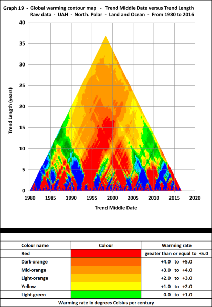
This is part 3 of my reply.
Have a look at my website:
mta-graphs.com
Look at all of the UAH and Gistemp global warming contour maps. See the similar patterns that are in most of them.
I have even made Gistemp ones for the same date range as the UAH ones, so that they are easy to compare.
If you want to copy and paste some of the images, so that you can directly compare different contour maps, then right-click, choose “View page source”, scroll to the bottom, and you will see the links to the graphs.
They look like this:
Right-click the link and choose “Open link in new tab”
If the link to the graph ends in “_d600.png” then you can usually get a bigger image by removing the “_d600”
Leave the “.png” in the link to the graph.
Frank,
This is part 4 of my reply.
The last post turned the example of a link into the actual image. I will try to show the actual link here:
The links look like this:
“https://storage.googleapis.com/wzukusers/user-21443138/images/58420d289f48bI7aJiDY/North-Polar-Land-and-Ocean_d600.png”
Right-click the link and choose “Open link in new tab”
If the link to the graph ends in “_d600.png” then you can get a bigger image by removing the “_d600”
Leave the “.png” in the link to the graph.
Just recently, in a rather lengthy exchanged with LOUMAYTREES, he was going on about a cooling trend in relation to co2. First, from at least 2000 I have never said that there wasn’t warming. What I disagreed with is the cause. Second, if anybody does look, there seems to be an underlying warming trend. However, it is nowhere as dramatic or conform to any of the models. He wasn’t about to get me suckered me into that argument.
The other issue is the adjusting the data. The actual warming may only 2/3 or 1/2 of what they are saying .
The very biggest problem is that so much of focus has been on proving AGW, that in a downturn there won’t be any way of explaining it. Or making any kind of informed opinion on it that would make a difference. The ramifications are enormous.
Using satellite data at least before the very recent change showed there was no underlying trend noticeable. The change in the AMO easily removes any trend in global temperatures over this period.
http://i772.photobucket.com/albums/yy8/SciMattG/RSS%20Global_v_RemovedAMO2_zpsssrgab0r.png
Any differences with surface data sets for example below were manufactured.
http://i772.photobucket.com/albums/yy8/SciMattG/NHTemps_Difference_v_HADCRUT43_zps8xxzywdx.png
Maybe, maybe not… I don’t know. I’m using the information I had at hand. For some reason they hadn’t adjusted it until recently.
I don’t know what they’ve done. No matter how you look at it, it’s bad science. More suited to a religious belief .
I have an idea, but I don’t know how valid it is, I do think there has been some warming, I disagree with the cause (AGW). The early 1970′ s were scary. It was scary because food production was down and world reserves were close to running out. Whether it was weather or climate, we had back to back super harvests. Farmers were being urged to plant ” fence post to fence post “. Loans were easy and because of the superharvest and the ban on selling grain to the Soviets ( Afghanistan) a lot of farmers started going bankrupt. The reaction wasn’t immediate, but concerts to help farmers, farm aid. And in song John Melloncamp’s blood on the plow. There was a meeting in Switzerland that helped push a lot more American farmers into bankruptcy as food supplies became more stable. I still have the documents, I consider it so important that it is in a safety deposit box in a bank.
What I know for sure is that they are lying, and hiding the information and process from the public eye. NOAA doesn’t want you to know or think anything different than what they are telling you.
There sure has been some warming, but by no underlying trend means after any natural contributions are taken into account.
A strong El Nino warms the Arctic for example later significantly, so for the example above to reduce the temperatures around the strong 1997/98 El Nino. When it was supposed to be accounted for by more Arctic coverage was nonsense.
They deliberately cherry picked warmed and cooled periods so perfect, it was obvious it was only bias confirmation by human tampering of data to support their agenda.
Thank you rishrac, for making my points from some time ago:
1. IPCC AR5 (CMIP5) climate models did not reflect the known lower temperatures during 2000-2005 in their hindcasts. Had they, their out-year forecasts would have had to be cooler.
2. IPCC AR5 (CMIP5) climate models ran so hot that AR5 had to adjust near-term (through 2035) forecasts downward because the models were so wacko hot.
3. IPCC AR5 kept the wildly hot CMIP5 model out-year forecasts to appease the politicians. The arm-waving used was risible.
It is my understanding that AR6 will simply accept AR5 warming conclusions and play games with negative assumptions about environmental impacts.
Maybe President The Donald’s appointees to the international climate follies will wack some dicks.
You’re welcome. They don’t show the 95% certainty anymore on the models… even with the adjusted temperatures they are far below the lowest modeled numbers.
Only two things missing form SkepticalScience
Skepticism has its little more than a fanzine of climate doom
and any science worth a dam .
Remember its love child of ‘Real Climate ‘ and Mann , set up to give an ‘alternative’ view to the climate ‘scientists’ on how great climate ‘scientists’ are and how they are never ,ever wrong . And a love child of that pair is one not even a mother could love .
The way you’ve shown the data does not give equal prominence to variation over different timescales. So, I wondered what would happen if it were shown more appropriately. the final result is as follows (rather hacked as I’m going to bed)
Article: http://scottishsceptic.co.uk/2016/12/09/a-colour-map-of-temperature-change/
Image
http://scottishsceptic.co.uk/wp-content/uploads/2016/12/curl1.png
John Cook”s SKS is really a psudo scientific political site dedicated to defending the AGW conjecture no matter what. Comments on their articles are sensored and many critical of the AGW conjectrure are deleted, At lease that had been by experiincing. Years ago I posted a comment over there that just demolished the AGW conjecture. They left it in because they did nto seem to understand it.
The believers of AGW are going to face reality which is it never has existed, existed or will going forward.
This is a theory in which the basic premises it was built on have failed to materialize , such as a decrease in OLR, a greater +AO evolving and the lower tropospheric hot spot missing in action.
This theory has wasted so much time in research in the studying of this ill conceived theory (AGW) which should have been devoted instead to what really causes the climate to change and it is not CO2.
I have wasted time studying this theory to some degree also.
The historical climate record shows this period of time in the climate is not unique, yet this theory lives on but I think the cooling which is now happening may end it .
“After all it is not as though the energy provided by the sun fluctuates like the spikes on the graphs”
So what makes it get warmer in the Spring? Increasing insolation. Smooth and uniform. But the warming isn’t.
The second triangle graph looks very much like a fractal. But it would – climate is chaotic. Local disorder, global order.
Anyway, if temperature data sets are stochastic, how can SkS overlay multiple trend lines on the graph? (AFAIK min & max data sets are not a signal, and cannot be treated as such, although that stuff is a bit advanced for me).
Karim Ghantous, December 8, 2016 at 10:49 pm … said:
The second triangle graph looks very much like a fractal.
Interesting you should say that, because looking at the tiny alarmist segment of the “escalator” and then at the “Holocene” epoch, and then at the geological-history, … I thought “embedded similarity”, you know, like in music, where overtones and undertones are embedded in the main frequency as self-similar, embedded cyclic patterns. [Am I straying into la-la-land-at-risk-of-being-deleted territory yet?]
When the Earth is going through a period of solar induced warming there will be a step up in temperatures from one positive ENSO phase to the next.
When the Earth is going through a period of solar induced cooling there will be a step down in temperatures from one negative ENSO phase to the next.
We are likely at the transition point between upward stepping and downward stepping.
Exactly Stephen
Right, except this is true with each and every possible cause, not just “solar induced”.
Meaning opposing the “escalator” and the “single straight” is nonsense.
What’s make the “escalator” relevant is just the fact that they ruled out the possibility of having a step 17y or more long. But it showed itself.
We don’t know enough of climate to be sure of any future. Could be going downward, or resume upward, or whatever.
What we do need, however, to falsify the sc4m, is that human keep dumping lots of CO2 in the atmosphere so. If CO2 stop going up despite that, the CAGW hypothesis is shown wrong. Likewise if temp stop going up, or even go down.
We may be unlucky, however.
paqyfelyc
Observing other parameters such as the timing of global albedo changes as per the Earthshine project relative to changes in solar activity should help to pin it down to solar changes.
Earlier Earthshine data from before 2000 showed declining
albedo until around 2000 and a slight recovery after 2000. I have now found data
for the period to date:
https://arxiv.org/pdf/1604.05880v1.pdf
See Figure 2
Overall, albedo has been roughly steady since 2000.
A plausible interpretation is that after 2000 the solar influence on the jet
stream tracks caused global albedo to recover from the pre 2000 low figures
which is what caused the current ‘pause’ in the global temperature trend.
To resume warming, global albedo needs to drop again and if albedo increases
further then cooling should commence.
The relatively weak solar cycle 24 has been able to cause the pause but it
seems that we may need an even weaker cycle 25 to increase albedo further to
tip the system into discernible cooling.
It is possible that the thermal inertia of the oceans has been sufficient to
delay the commencement of cooling which might otherwise have already
commenced at the current level of albedo.
Stephen Wilde on December 9, 2016 at 4:02 am
When the Earth is going through a period of solar induced warming there will be a step up in temperatures from one positive ENSO phase to the next.
When the Earth is going through a period of solar induced cooling there will be a step down in temperatures from one negative ENSO phase to the next.
Wow! Is this
– a theory
– a claim
– a supposition ?
Maybe you had this impression when comapring UAH and ENSO for the period 1997-2016…
But a look at a chart comparing temperatures with ENSO signals for the period 1979-2016
http://fs5.directupload.net/images/161209/7qc384xi.jpg
shows that you are a bit wrong (because you ignore for example volcanic forcings aka stratospheric aerosols). Some periods might let you indeed imagine it goes that way.
And a look at a similar chart for 1871-2016
http://fs5.directupload.net/images/161209/gnpx85yg.jpg
should convince you that your assumption does not reflect reality. The temperature response to MEI over 150 years is simply too random.
How accurate is HadCRUT4 ?
How accurate are
– MEI?
– UAH?
you made the wrong comparison graph: the escalator says something else then your graph.
you forget that la nina is not the opposite of el nino. even if this graph is ocean only, adding land surface to it doesn’t change it.
el nino’s are discharges of warm water which then remain lingering around, while la nina’s are recharges of the warm pool where El nino originates from
that means la nina’s do not discharge cold waters unlike el nino does.
that’s a big difference that seems to be forgotten a lot in the ENSO debate. this means that each big el nino is able to ramp up the temperature if they follow in good sequence
like this back to back la nina’s can hold a brake on the el nino.
then to finish there is maybe a correlation with ENSO and PDO, but that’s not known in what way and how it works. that part is still heavily debated.
i’m pretty sure that if we had accurate el nino data in the first warming period and cooling period we would see a similar escalator…
forgot to add: we do see since 1975 a sudden change from ENSO turning from more “la nina state” to more “el nino state” In the way ENSO works we now do see a discharge of the heat stored in the warm pool from the late 40’s till mid 70’s.
Maybe that this correlates with the most recent warming is just coincidence?
Frederick,
El Nino releases warmth to the atmosphere over and above that from incoming solar energy.
La Nina reduces warming of the atmosphere by diverting incoming solar energy to the recharge process.
In thermal terms as far as the air is concerned they are opposites.
Over the period MWP to LIA I would expect that La Ninas became dominant relative to El Ninos and since the LIA it has been the opposite.
I rely only on satellite data and, sadly, we only have that since 1979 but for that period my proposal holds good.
Even Judith curry did do a nice follow up on this by writing an interesting article about it: how El nino and La nina do “add up” and comparing it to the global temperature….
article of Judith curry
i agree that you can say that for the thermal terms of air they are “opposite”.
“forgot to add: we do see since 1975 a sudden change from ENSO turning from more “la nina state” to more “el nino state” In the way ENSO works we now do see a discharge of the heat stored in the warm pool from the late 40’s till mid 70’s.
Maybe that this correlates with the most recent warming is just coincidence?”
Not a coincidence when it can easily be seen the solar energy ramped up between the 1940’s and 1960’s. The atmosphere was unable to see this change quickly because numerous La Nina’s kept it away from the surface until later. Later in the 1970’s the Pacific Ocean shift change occurred and the warm AMO came with it.
The difference in warmth recently compared to the warming up to the 1940’s was higher solar activity and the AMO/PDO both being positive at the same time with more El Nino’s of course.
The MEI is now useless for comparing with global temperature trends because they already assume global warming is causing the higher NINO 3 and NINO 4 SST’s. Unfortunately so they adjusted it recently to take this into account. It is very unscientific and very on the assumption side with no evidence El Nino’s having anything to do with humans.
“Do they expect us to believe that global warming proceeds at a uniform constant rate?”
Yes – because CO2 is increasing at a mostly uniform and constant rate since the industrial revolution. For their theory to hold true, the only reason for any increase in mean global temperatures must be mankind’s release of CO2 into the atmosphere. Which on its face value is laughable that the entire climate of the Earth hinges solely on CO2 levels.
They believe it. Clearly.
John Cook deleted my Escalator Gif from the escalator thread on SkS, then he deleted my SkS account, then he wrote a polite email asking me who created it? When I told him I did he told me not to bother trying to comment at SkS again.
Touched a nerve I did
In my experience, warmist blogs censor posts that disagree with them
Pseudo skeptical pseudo scientific site. I’ve met their climate warriors on facebook. They are really brainwashed and very aggressive. They deny logic, they deny physics, they deny the scientific method, they deny everything that’s against their religious doctrine. I quickly learned to put them on ignore, one cannot have a rational discussion with them 🙂
I have also had a less than worthwhile experience on their psudosceintific, political, AGW religious site. It is amayzing what they will allow in terms of comments if you start it off in such a way that you appear to be agreeing with them. I was able to post one comment that just blew away AGW if one bothered to read the whole thing. Maybe they have actually discovered and deleted it by now.
The pretty triangle is not so helpful. Instead, financial graphing may offer what this author is looking for.