This is a guest essay by Mike Jonas, part 1 of 4
Introduction
The aim of this article is to provide simple mathematical formulae that can be used to calculate the carbon dioxide (CO2) contribution to global temperature change, as represented in the computer climate models.
This article is the first in a series of four articles. Its purpose is to establish and verify the formulae, so unfortunately it is quite long and there’s a fair amount of maths in it. Parts 2 and 3 simply apply the formulae established in Part 1, and hopefully will be a lot easier to follow. Part 4 enters into further discussion. All workings and data are supplied in spreadsheets. In fact one aim is to allow users to play with the formulae in the spreadsheets.
Please note : In this article, all temperatures referred to are deg C anomalies unless otherwise stated.
Global Temperature Prediction
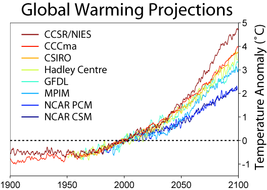
The climate model predictions of global temperature show on average a very slightly accelerating increase between +2 and +5 deg C by 2100:

We can be confident that all of this predicted temperature increase in the models is caused by CO2, because Skeptical Science (SkS) [6], following a discussion of CO2 radiative forcing, says :
Humans cause numerous other radiative forcings, both positive (e.g. other greenhouse gases) and negative (e.g. sulfate aerosols which block sunlight). Fortunately, the negative and positive forcings are roughly equal and cancel each other out, and the natural forcings over the past half century have also been approximately zero (Meehl 2004), so the radiative forcing from CO2 alone gives us a good estimate as to how much we expect to see the Earth’s surface temperature change.
[my emphasis]
So, if we can identify how much of the global temperature change over the years from 1850 to present was contributed by CO2, then we can deduce how much of the temperature change was not. ie,
T = Tc + Tn
where
T is temperature.
Tc is the cumulative net contribution to temperature from CO2. “CO2” refers to all CO2, there is no distinction between man-made and natural CO2.
Tn is the non-CO2 temperature contribution.
Obviously, all feedbacks to CO2 warming (changes which occur because the CO2 warmed) must be included in Tc.
CO2 Data
The Denning Research Group [4] helpfully provide an emissions calculator, which shows CO2 levels and the estimated future temperature change that it causes under “Business as usual” (zero emission cuts) :

Cross-checking the future warming in this graph against Figure 1, the CO2 warming from 2020-2100 is just under 3.5 deg C compared with about 3.25 deg C model average in Figure 1. That seems close enough for reliable use here. But data going back to at least 1850 is still needed.
There is World Resources Institute (WRI) CO2 data from 1750 to present [3], and CO2 data measured at Mauna Loa from 1960 to present [5]. Together with the Denning “Business as usual” CO2 predictions above, the CO2 concentration from 1750 to 2100 is as follows :

For dates covered by more than one series, the Mauna Loa measured data will be preferred, then the WRI data.
Because the “pre-industrial” CO2 is put at 280ppm [6], and the data points in the above graph before 1800 are all very close to 280ppm, a constant level of 280ppm will be assumed before 1800.
CO2 Contribution
The only information still needed is the CO2-caused warming before about 1990.
A method for calculating the temperature contribution by CO2 is given by SkS in [6] :
dF = 5.35 ln(C/Co)
Where ‘dF’ is the radiative forcing in Watts per square meter, ‘C’ is the concentration of atmospheric CO2, and ‘Co’ is the reference CO2 concentration. Normally the value of Co is chosen at the pre-industrial concentration of 280 ppmv.
dT = λ*dF
Where ‘dT’ is the change in the Earth’s average surface temperature, ‘λ’ is the climate sensitivity, usually with units in Kelvin or degrees Celsius per Watts per square meter (°C/[W/m2]), and ‘dF’ is the radiative forcing.
So now to calculate the change in temperature, we just need to know the climate sensitivity. Studies have given a possible range of values of 2-4.5°C warming for a doubling of CO2 (IPCC 2007). Using these values it’s a simple task to put the climate sensitivity into the units we need, using the formulas above:
λ = dT/dF = dT/(5.35 * ln[2])= [2 to 4.5°C]/3.7 = 0.54 to 1.2°C/(W/m2)
Using this range of possible climate sensitivity values, we can plug λ into the formulas above and calculate the expected temperature change. The atmospheric CO2 concentration as of 2010 is about 390 ppmv. This gives us the value for ‘C’, and for ‘Co’ we’ll use the pre-industrial value of 280 ppmv.
dT = λ*dF = λ * 5.35 * ln(390/280) = 1.8 * λ
Plugging in our possible climate sensitivity values, this gives us an expected surface temperature change of about 1–2.2°C of global warming, with a most likely value of 1.4°C. However, this tells us the equilibrium temperature. In reality it takes a long time to heat up the oceans due to their thermal inertia. For this reason there is currently a planetary energy imbalance, and the surface has only warmed about 0.8°C. In other words, even if we were to immediately stop adding CO2 to the atmosphere, the planet would warm another ~0.6°C until it reached this new equilibrium state (confirmed by Hansen 2005). This is referred to as the ‘warming in the pipeline’.
Unfortunately, not enough exact parameters are given to allow the temperature contribution by CO2 to be calculated completely, because the effect of ocean thermal inertia has not been fully quantified. But it should be reasonable to derive the actual CO2 contribution by fitting the above formulae to the known data and to the climate model predictions.
The net radiation caused by CO2 is the downward infra-red radiation (IR) as described by SkS, less the upward IR from the CO2 warming already in the system (CWIS). This upward IR will be proportional to the fourth power of the absolute (deg K) value of CWIS [9]. The net effect of CO2 on IR is therefore given by :
Rcy = 5.35 * ln(Cy/C0) – j * ((T0+Tcy-1)^4 – T0^4)
where
Rcy is the net downward IR from CO2 in year y.
Cy is the ppm CO2 concentration (C) in year y.
C0 is the pre-industrial CO2 concentration, ie. 280ppm.
j is a factor to be determined.
T0 is the base temperature (deg K) associated with C0.
Tcy is the cumulative CO2 contribution to temperature (Tc) at end year y, ie, CWIS.
SkS [6] says “it takes a long time to heat up the oceans due to their thermal inertia”. On this basis, CWIS is presumably in some ocean upper layer.
For a doubling of CO2, in the absence of other natural factors, the equilibrium temperature increase using the SkS formula is 5.35 * ln(2) * λ where λ = 3.2/3.7 (assuming a mid-range equilibrium climate sensitivity (ECS) of 3.2).
At equilibrium, Rc = 0. For ECS = 3.2, j can therefore be determined from
0 = 5.35 * ln(2) – j * ((T0+3.2)^4 – T0^4)
hence
j = (5.35 * ln(2)) / ((T0+3.2)^4 – T0^4)
Because “the natural forcings over the past half century have also been approximately zero” [6], the SST should be a reasonably good guide to CWIS. The global average SST 1981 to 2006 was 291.76 deg K [8]. Subtracting the year 1993 Tc of 0.7 (from the Denning data [4]) gives T0=291 deg K. Hence j = (5.35 * ln(2)) / ((291+3.2)^4 – 291^4) = 1.16E-8 (ie. 1.16 * 10^-8, or 0.0000000116).
Using the formula
δTcy = k * Rcy
where
δTcy is the increase (deg C) in CWIS in year y.
k is the one-year impact on temperature per unit of net downward IR.
the value of k can be found which gives a future temperature increase matching that of the climate models, ie. 3.25 deg C from 2020 to 2100. A reasonability check is that the result should closely match but be slightly lower than the Denning warming calculation in Figure 2 (lower graph) (slightly lower because target is 3.25 deg C not 3.5) …..

….. it does, for k = 0.02611 (the graph for 3.5 deg C is also shown in [7]). [Note that the calculated warming is “anchored” at 1750 T=0, and that the shape is determined only by the formula so there is no guarantee that the 2020 and 2100 temperatures will be close to the Denning temperatures. ie, this is a genuine test.].
Note: At this rate, global temperature takes 52 years to get 80% of the way to equilibrium (as in “equilibrium climate sensitivity”), 75 years to reach 90%, 97 years to reach 95%, 148 years to reach 99%.
The above formula can therefore reliably be used for CO2’s contribution to global temperature since 1750.
1850 to 2100
The above formulae can now be applied to the period 1850 – 2100, to see how much has been and will be contributed to temperature by CO2.
For temperature data 1850 to present, Hadcrut4 global temperature [1] is used. For future temperatures, the formula warming (as in Figure 4) is used.

Applying the above formulae shows the contributions to temperature by CO2 and by other factors :

As expected,
· the dominant contribution is from CO2,
· other factors contribute the inter-annual “wiggles” and virtually nothing else.
Note : The contribution to global temperature by CO2 is only man-made to the extent that the CO2 is man-made. As stated earlier, no distinction is made between man-made CO2 and natural CO2. Obviously, all pre-industrial CO2 was in fact natural. Similarly, for the non-CO2 contribution, no distinction is made between natural factors and non-CO2 man-made factors (such as land-clearing, for example), but the non-CO2 factors are thought to be predominantly natural. The feedbacks from the CO2 warming as claimed by the IPCC (eg. water vapour, clouds) are included in the CO2 contribution above.
Conclusion
The picture of global temperature and its drivers as presented by the IPCC and the computer models is one in which CO2 has been the dominant factor since the start of the industrial age, and natural factors have had minimal impact.
This picture is endorsed by organisations such as SkS and Denning. Using formulae derived from SkS, Denning and normal physics, this picture is now represented here using simple mathematical formulae that can be incorporated into a normal spreadsheet.
Anyone with access to a spreadsheet will be able to work with these formulae. It has been demonstrated above that the picture they paint is a reasonable representation of the CO2 calculations in the computer models.
The next articles in this series will look at applications of these formulae.
Footnote
It is important to recognise that the formulae used here represent the internal workings of the climate models. There is no “climate denial” here, because the whole series of articles is based on the premise that the climate computer models are correct, using the mid-range ECS of 3.2.
See spreadsheet “Part1” [7] for the above calculations.
Mike Jonas (MA Maths Oxford UK) retired some years ago after nearly 40 years in I.T.
References
[1] Hadley Centre Hadcrut4 Global Temperature data http://www.metoffice.gov.uk/hadobs/hadcrut4/data/current/time_series/HadCRUT.4.3.0.0.annual_ns_avg.txt (Downloaded 20/5/2015)
[2] Climate model predictions from http://upload.wikimedia.org/wikipedia/commons/a/aa/Global_Warming_Predictions.png (Downloaded 20/5/2015) Note: Wikipedia is an unreliable source for contentious issues, but for factual information such as the output of computer models, and in the context for which it is being used here, it should be OK.
[3] CO2 data from 1750 to date is from World Resources Institute http://powerpoints.wri.org/climate/sld001.htm (Downloaded 20/5/2015. Digitised using xyExtract v5.1 (2011) by Wilton P Silva)
[4] Emissions calculator from Denning Research Group at Colorado State University http://biocycle.atmos.colostate.edu/shiny/emissions/ using no emissions cuts, ie, “Business as usual”. (Downloaded 20/5/2015. Digitised using xyExtract v5.1 (2011) by Wilton P Silva)
[5] Mauna Loa CO2 data from http://scrippsco2.ucsd.edu/data/flask_co2_and_isotopic/monthly_co2/monthly_mlf.csv (Downloaded 27/2/2012)
[6] Skeptical Science 3 Sep 2010 http://www.skepticalscience.com/Quantifying-the-human-contribution-to-global-warming.html (As accessed 20/5/2012).
[7] Spreadsheet “Part1” with all data and workings . Part1 (Excel .xlsx spreadsheet)
[8] Spreadsheet “SST” SST (Excel .xlsx spreadsheet)
[9] Stefan-Boltzmann law. See http://hyperphysics.phy-astr.gsu.edu/hbase/thermo/stefan.html
Abbreviations
AR4 – (Fourth IPCC report)
AR5 – (Fifth IPCC report)
CO2 – Carbon Dioxide
CWIS – CO2 warming already in the system
ECS – Equilibrium Climate Sensitivity
IPCC – Intergovernmental Panel on Climate Change
IR – Infra-red (Radiation)
LIA – Little Ice Age
MWP – Medieval Warming Period
SKS – Skeptical Science (skepticalscience.com)
WRI – World Resources Institute
“The net effect of CO2 on IR is therefore given by :
Rcy = 5.35 * ln(Cy/C0) – j * ((T0+Tcy-1)^4 – T0^4)”
It looks very scientific, but there is a lot of basic physics missing. Are all these “T”s day temperatures, night tempearures, summer temperatures, or winter temperatures? Has the author seen formulas taking into account the Earth’s rotation, inclination, and orbit eccentricity?
That’s where a true science would start, not at a simplified model of an unknown quality.
It will be interesting to see where this goes. Another ‘simple model’ that generally reproduces GCM results using mainstream warmunist inputs and relationships. Presumably will be pressure tested.
There is already one ‘finding’ in part 1 that prompts an observation. Figure 6 deduces that Tn is roughly net zero. That is, no net natural variation. The computational period is roughly 1850-2010, 160 years, or roughly two 70-80 year full ‘cycles’ of some amplitude ‘sine wave’ natural variation. The early DMI arctic ice records, plus the DMI recent Arctic ice and Greenland ice mass balance data, hint at such a cycle. Moreover, having recently bottomed, with ice now on the upswing. With about that periodicy.
Plainly, on longer time intervals there is natural variation (MWP, LIA). Still Net Tn zero around the overall cooling trend from Holocene optimum? Dunno if paleoproxies have enough resolution to attempt the analysis.
Plainly, on shorter 30-40 year intervals natural variation does matter even if the full cycle Tn is roughly net zero. Even AR4 said so in discussing ~1920-1945, then ~1945-1970. BUT, the CMIP5 GCMs were parameterized to hindcast well from 2006 back to about YE1975, and under the ‘ Meehl assumption’ of little natural variation. Ergo, CMIP5 should run hot compared to the Tn downcycle portion–that is to somewhen in the 2030s. And GCMs have been doing just that since about 2000. These musings at least seem to fit loosely together.
I’m working on my Ph.D. in mathemanics.
T = Tc + Tn is wrong T = Tc + Tn +Tcn where Tcn is the temperature increase or decrease due to the interaction between c & n.
Your concept of Tcn is basically the CO2 feedbacks. I have been careful to build them all into Tc. So my Tc is your (Tc + Tcn).
Mike, consider a simple world with no atmosphere and where only albedo and CO2 can change. Add some CO2 and you get a Tc value. Instead of adding CO2 let the albedo change so less light is reflected and you get a Tn but let both happen and the new temperature difference is not Tc+Tn and there is no feedback ie CO2 doesn’t affect albedo and albedo doesn’t affect CO2. There is an entanglement because of the T^4 law of Boltzmann. Are you sure it is valid to simply adjust the Tn to a different value and then continue to use it for further calculations?
Very good point, and hopefully I have avoided any pitfall here. Tc gets used in further calculations, but Tn does not.
All this still leaves the question as to what caused the medieval warming period
Part 2.
While we are talking co2 maths, can someone explain why human emissions have sped up in recent decades but the official rise in co2 stays consistent? Seems obvious some mechanism isn’t even hinted at yet let alone explained. Unless of course it is something other then humans driving up co2 levels.
Randy, glad to hear you ask that question. It is temperature and NOT human emissions that drive carbon growth. Carbon growth and temperature have been in lock step since the inception of the mauna loa data set (this is southern hemisphere land data which does not pick up the early 90s cooling due to pinatubo which is located at 15 degrees north latitude):
http://www.woodfortrees.org/plot/esrl-co2/from:1959/mean:24/derivative/plot/hadcrut4sh/from:1959/scale:0.22/offset:0.10
This still does not answer the crucial question of whether or not the rise is natural or anthropogenic. If it’s natural then perhaps henry’s law; if anthropogenic then temperature is causing an inefficiency in the carbon sinks as temps rise…
Test one, two…
Climate models still use a CO2 annual growrth rate of about 1%, which is supposed to approximate emmissions growth. However CO2 content has only been growing about half as much. So their forecasts of future warming are too pessimistic (not counting that their climates sensitivity is also too high). So apparently the oceans and forests are absorbing about one half of the emissions. The oceans would be absorbing a little more if they has not warmed a little. The forests should be absorbing more with time because of the increasing CO2 causing faster tree growth.
“…the whole series of articles is based on the premise that the climate computer models are correct, using the mid-range ECS of 3.2.”
You know, if Equilibrium Climate Sensitivity [ECS] means a doubling of CO2 produces 3.2° of warming and that the logarithmic doubling starts at around 10 – 20 parts per million, then CO2 is around 45% of the green house effect if the green house effect is 33°.
Hi Steve; at 400 ppm the total CO2 column represents about 3000 abs. The line centre saturates by about 2 abs (99% absorption) which is more or less where the logarithmic relationship starts so we are somewhere between 10 and 11 doublings into saturation. If the total CO2 column absorbs about 30 watts/sqM it would seem that that each doubling would contribute around 3 watts/sqM. Now the sensitivity of earth in watts/sqM/C is normally quoted at around 3.7 watts/sqM/C so that would suggest the direct impact of doubling CO2 is somewhere around 0.8C -1C. The rest is feedbacks but that raises an interesting question – in almost all naturally stable systems (and climate is certainly a naturally stable system) feedbacks are negative. Indeed negative feedback is more or less a mandatory prerequisite for stability so the claim of not just positive feedback but massive positive feedback is truly extraordinary. The only evidence for it that I have seen is the prediction of a hotspot in the upper tropical troposphere – you know, the one that 1000’s of balloon flights can’t find any trace of!
λ = dT/dF = dT/(5.35 * ln[2])= [2 to 4.5°C]/3.7 = 0.54 to 1.2°C/(W/m2)
We currently get an avearge of a little less than 240 watts/square meter from the sun.
Plugging in that 1.2 C(W/m2) gives 240*1.2 = 288 K, the current average temperature at earth’s surface.
Since radiation is proportional to the 4th power of the temperature, it’s SILLY to assume that last 3.7 watts will have anywhere NEAR the effect of the AVERAGE for 240 watts.
At this site, Nir Shaviv calculate a sensitivity of about 0.21 C (W/m2)
http://www.sciencebits.com/OnClimateSensitivity
And I suspect that even THAT is on the high side. I think what Nir Shaviv is actually calculating is
the effective temperature change if the sun increased its radiation in all wavelengths proportionally,
so earth would get an average of about 243.7 watts rather than the 240 average we currently get.
Using multilayer greenhouse models like
https://en.wikipedia.org/wiki/Idealized_greenhouse_model
or
http://www.geo.utexas.edu/courses/387h/Lectures/chap2.pdf
in actuality we’d be adding a fractional 3.7 watt layer to our current atmosphere, increasing surface
wattage from an average of 390 watts to 393.7 watts, giving an increase of 0.7 C and a sensitivity of
aboout 0.189 C(W;m2). Of course, our surface currently gets around 490 watts, but 100 watts of that
results in evaporation and convection, and doesn’t go into sensible heat. If a similar fraction of the 3.7 Watt increase ALSO goes into evaporation and convection, that reduces the sensitivity to about
0.189*(390/490)= 0.15 C(W/m2), what I consider to b a much more plausible figure than even Nir Shaviv gives.
OK, thanks for clarifying the wavenumber vs wavelength issue. Here is another question, using wavelength or wavenumber. Here is a chart of CO2’s absorption of IR under different concentrations. What % of the entire radiation from the earth does this increase represent? If we increase CO2 by a factor of 4, is that a material change in absorption given that H2O also absorbs those wave lengths.
http://members.casema.nl/errenwijlens/co2/co205124.gif
http://i787.photobucket.com/albums/yy154/RichardDH/AGW/emitt.jpg
http://earthobservatory.nasa.gov/Features/Iris/Images/greenhouse_gas_absorb_rt.gif
Is this chart correct? Is CO2 relatively transparent at 15 microns/666 wavenumber?
http://www.ar15.com/media/mediaFiles/1334/37782.GIF
http://bradleydibble.authorsxpress.com/files/irCO2.jpeg
In a word. YES. The 666 line seems to be overstated as it is. It really is a quite weak line. Very often, in IR spectroscopy, things are arranged such that strong lines are way saturated, so that the weak lines will show up and their wavenumber can be determined. When the system is adjusted so the strong lines are on scale properly, the weak lines are not even a bump on the baseline. Unless you already know, you would not even suspect they are there. This practice of generating distorted spectra is OK for most things, but is a disaster for quantitative work. As a result, there has been much confusion about the true relative intensities of IR lines.
BTW: The 15 micron line is 665 wavenumbers. It was informally changed to 666, from biblical reference, The Number Of The Beast. That made CO2 “The Molecule Of The Beast”. It seemed all too fitting when CAGW came along (much later). Some of us have been snickering ever since.
6 protons
6 neutrons
6 electrons
This cannot be a coincidence !!!
…. carbon that is, of course.
Is the absorption band then at 15 microns CO2 or H2O or Both?
http://earthobservatory.nasa.gov/Features/Iris/Images/greenhouse_gas_absorb_rt.gif
@ur momisugly phil:
Everything in science happens for a reason, creepy how this works.
@ur momisuglyco2islife:
Yes, the absorption band will be the sum of both contributors.
In spite of what is implied by the graphic, I suspect the water vapor dominates by far. Water, is after all, a very good absorber in the IR and there is a lot more of it. Water vapor is given as 2% – 5% of the atmosphere (CRC Handbook) which is 20,000ppm – 50,000ppm, compared to CO2 at 400ppm.
Just to underline the point, experimentally water is a huge pain in the IR lab. When collecting spectra, the samples have to be dry, dry, dry. Any solvents used have to be dry, dry, dry. And that can be a real challenge, depending on the solvent. Water absorbs strongly across the entire spectrum. Any water contamination will cause a big absorption band which will blot out any spectral features you are trying to see. In addition, the instruments have to be kept in low humidity climate controlled lab rooms. The whole water issue can be a huge PITA in IR land.
Nobody ever said “Watch out for CO2 contamination”.
@Phil
The Atom Of The Beast
Is the absorption band then at 15 microns CO2 or H2O or Both?
Both, but as you will see from the spectrum below, CO2 dominates.
http://i302.photobucket.com/albums/nn107/Sprintstar400/H2OCO2.gif
The top spectrum is H2O the bottom one CO2.
??? 15 micron is EXACTLY 666.66666… wavenumbers. But the peak (the Q branch) is actually at about 670 wavenumbers, so not exactly 15 micron.
Why not just look at top of the atmosphere spectrograms and stop “suspecting”? Water vapor often does “dominate”, but not for the most part in the bite taken out by CO2. The bite taken out by CO_2 is a) absolutely real and in pretty much all spectrographs no matter which part of the Earth you look at from the TOA; b) up against water vapor on one side, but the water vapor part goes up and down with the humidity. And water vapor has effects elsewhere in the spectrograph, not just on the long wavelength side of the LWIR curve. So do clouds.
The fact that water vapor dominates, especially in the tropics and over the ocean, does not mean CO_2 has no effect in either place. CO_2’s relative effect is greatest over the poles and desert (where it is usually/often dry) but its effect is zero nowhere.
Hi CO2islife; I posted a comment at 2:44 16th July which partly answers your question (just above) but to answer this issue in more detail, how much difference does raising CO2 conc make. Once the line center saturates further absorption occurs though increasing width of the absorption line and that is a logarithmic relationship (the line profile is close to gaussian and squaring a gaussian (ie: doubling concentration) yields a new gaussian with a larger sigma). As to whether the plot of CO2 absorption you showed is correct – yes it looks like it. CO2 has three very large absorption peaks at 2.7 microns 4.3 microns and 14.7 microns (3700 wavenumbers, 2300 wavenumbers and 665 wavenumbers approximately) All 3 can be seen on the plot. The 4.3 micron peak is the strongest but the other 2 are also very large. (This plot is probably for very low concentration CO2 over a short path length so the notches don’t go all the way to zero). However the Earth is not warm enough to emit significant energy at 2.7 or 4.3 microns so there is no significant energy at those wavelengths for the CO2 to absorb. The 14.7 micron peak is the important one and it is VERY strong relative to the amount of CO2 in the atmosphere. Even an atmospheric concentration of around 0.3 ppm would be enough to absorb all the energy radiated by earth’s surface at 14.7 microns. Your point about water vapour is very relevant. On the short wavelength side CO2 runs up against the atmospheric window so its impact is significant but at the long wavelength side it buts up against water vapour absorption. That means on the long wavelength side it is just absorbing energy that would anyway be absorbed by water vapour (well most of it, CO2 absorption seems to be somewhat stronger than the water vapour absorption). That would mean the apparent impact is close to halved.
Michael Hammer, you say: “Even an atmospheric concentration of around 0.3 ppm would be enough to absorb all the energy radiated by earth’s surface at 14.7 microns.” and “Once the line center saturates further absorption occurs though increasing width of the absorption line and that is a logarithmic relationship”. So at 14.8 microns a lot more than 0.3 ppm will be required to absorb all the emitted energy at that wavelength, and even more CO2 at 14.9 microns, etc.
As 14.7 microns is a point, presumably this is shorthand for “14.65 to 14.75”?
Are these statements correct? Just to clarify my thoughts – and perhaps help those others here who are not atmospheric physicists or spectrologists.
And Mike Jonas, in the article you quote SkS as saying:
“Plugging in our possible climate sensitivity values, this gives us an expected surface temperature change of about 1–2.2°C of global warming, with a most likely value of 1.4°C. However, this tells us the equilibrium temperature. In reality it takes a long time to heat up the oceans due to their thermal inertia. For this reason there is currently a planetary energy imbalance, and the surface has only warmed about 0.8°C. In other words, even if we were to immediately stop adding CO2 to the atmosphere, the planet would warm another ~0.6°C until it reached this new equilibrium state (confirmed by Hansen 2005). This is referred to as the ‘warming in the pipeline’.”
The warming should be, say, 1.4C but it is only 0.8C. SkS attributes this to the inertia of the oceans which will eventually catch up and raise the warming by 0.6C to 1.4C, to make the earth correspond to the models. To do this the oceans would have to be warmer than they are, and they would cool, releasing energy to the atmosphere and the earth, to raise the observed temperature. This is totally in contradiction to: “In reality it takes a long time to heat up the oceans due to their thermal inertia.” which implies, at least to me, that the oceans have not materially warmed up yet. This also implies to me, that “if we were to immediately stop adding CO2 to the atmosphere” the result would be a COOLING by, perhaps 0.6C. Has no one picked this up before – surely I am not the first to have noticed this contradiction in the SkS argument – though I fancied that RichardsCourtney was about to do so in his post of “July 25, 2015 at 12:45 pm”. Without actually stating this was a contradiction, he correctly stated that this discrepancy had destroyed any resemblance of the Model World to the Real World
Is the absorption band then at 15 microns CO2 or H2O or Both?
Phil.: “Both, but as you will see from the spectrum below, CO2 dominates.”
What are the respective concentrations you are using for these comparisons?
At current concentrations, H2O mostly overlaps CO2 ~15um band absorption/emission:
http://1.bp.blogspot.com/_nOY5jaKJXHM/TJe36s1JB0I/AAAAAAAABTE/kgD4VUKlyu0/s400/Fullscreen+capture+9202010+123527+PM.jpg
A spectrum at such low resolution doesn’t allow for a correct interpretation, as shown at high resolution there are many more lines in the CO2 spectrum and the few H2O lines fall in-between the CO2 lines.
Phil, as I asked above, what are the respective concentrations of water vapor and CO2 in your comparisons?
A few more questions.
1) If CO2 absorbs 100% of IR at 15 Microns, why does the earth transmit 50% at 15microns.
2) why does the CO2 band widen when CO2 remains 400 PPM?
3) Why does a CO2 window develop over the Antarctic, where CO2 no longer absorbs even though it is 400 PPM?
http://members.casema.nl/errenwijlens/co2/spectra.gif
CO2 does not accumulate in the atmosphere. It flows like a river.
Outside a physics text, the best single source of IR science relating to GHE is at
http://www.barrettbellamyclimate.com/index.htm
Note especially the MODTRAN sections.
A more specific answer to your direct question is at
http://www.john-daly.com/artifact.htm
Generally, CO2 adds nothing at all to the waterworld of Earth, the GHE is entirely water.
Adding CO2 is overwhelmingly beneficial to surface biology, plants and crop growth, especially in dry areas.
What a great site – thanks (the barrettbellamy link).
1. Water is not saturated.
2. Pressure broadening.
3.Please explain this CO2 window over the Antarctic.
1) If CO2 absorbs 100% of IR at 15 Microns, why does the earth transmit 50% at 15microns.
All of the 15 micron IR from the Earth’s surface is absorbed (~190 units as shown on curve a), at an altitude corresponding to a temperature of about 220K the atmosphere has become sufficiently thin that emissions from the CO2 there is able to escape to space (~50 units).
2) why does the CO2 band widen when CO2 remains 400 PPM?
I’m not sure what you’re referring to here.
3) Why does a CO2 window develop over the Antarctic, where CO2 no longer absorbs even though it is 400 PPM?
There is a temperature inversion over antarctica, so the air at altitude is actually warmer than the surface, hence the bump above the surface emission is due to CO2 emissions from the warmer atmosphere. Note the ‘spike’ on the top of the ‘bump’ corresponding to the Q-branch of the CO2 spectrum.
That is exactly what I thought. How then does CO2 warm the lower atmosphere? How does warming the stratosphere result in warming the lower troposphere? Also, my understanding is that there is no stratospheric hotspot.
Also, the ocean are warming. How does CO2 warm the oceans?
co2islife asks “1) If CO2 absorbs 100% of IR at 15 Microns, why does the earth transmit 50% at 15microns.”
The postulate and the question are imprecisely stated. CO2 absorbs and then re-emits infrared; the energy does not remain absorbed. A carbon-dioxide laser depends on this phenomenon for its operation. Thus it is better for understanding that CO2 retards or delays radiative energy transport; how long it takes for energy to go a particular distance. Furthermore, CO2 that has absorbed a photon might deliver that energy in a physical collision imparting the head mechanically rather than re-radiating a photon. The opposite mechanism also exists; it might pick up thermal energy mechanically and emit a photon which is more likely the mechanism at the top of atmosphere.
It is also the case that CO2 can only absorb a photon that impinges upon it; hence the mean path length of a photon depends a great deal on the absolute density of CO2 molecules. I use 10 meters as the mean path length, your mileage may vary. What that means is that 10 meters above the surface of the earth, half of the radiative energy that could be captured by CO2 has already been captured. Of that, 1/2 will re-radiate back down, the other half re-radiate back up. Of the 1/2 radiated down, which is 1/2 of the surface radiation, 1/2 will actually succeed in reaching the surface. That’s 1/8th. So it is that carbon dioxide is a “blanket” that reduces the net radiation because some of it (but not very much) is coming back atcha.
The other GHG’s operate in similar manner.
I do not understand your other two questions.
This chart shows 3K mean path length (In think). I think it shows that the first 3K water vapor dominates, and its impact falls with altitude, which make sense given that it most likely condenses out or freezes. If I’m reading the chart correctly, it looks like you have to get at least 6K in the atmosphere before H2O falls enough for CO2 to have a material impact. Is my reading of this chart correct? If I am, how can CO2 be blamed for the lower atmosphere warming?
http://www.hashemifamily.com/Kevan/Climate/Earth_Atmosphere.gif
Low in the atmosphere vibrational energy of an excited CO2 molecule is predominantly transmitted to the surrounding atmosphere by collisions not emissions.
Hi again CO2is life. Your questions are both very relevant and very insightful. For a GHG its absorptivity and emissivity at the same wavelength must be identical (can be proven that if that were not the case a cold body could warm a wamer body). That means while CO2 absorbs at 14.7 microns it also emits at 14.7 microns according to its temperature (as defined by Planks law). Thus CO2 throughout the atmosphere is simultaneously absorbing and emitting energy at 14.7 microns. Only the last 2 abs (the very top of the GHG column) can emit to space, the rest of the emission from CO2 throughout the atmosphere is re-absorbed by the gas above or below. For CO2 the top of the gas column seems to be at the tropopause or more accurately the lower stratosphere. Thus what CO2 does is to absorb 14.7 micron surface emission (288K) and replace it with emission from a black body (at 14.7 micron) at the temperature of the tropopause (220K).
As CO2 concentration increases this occurs over a slightly larger range of wavelengths. As to why there is no notch in the antarctic (your CO2 window) its because the temperature of the lower stratosphere (or tropopause) is actually warmer than the surface. CO2 still absorbs all surface emission and replaces it with tropopasue emission but now the tropopause temperature is warmer so the emission at 14.7 microns is increased not decreased. IE: CO2 at the poles cools the earth it does not warm it but the effect is minor compared to the warming it creates elsewhere. A very good observation on your part.
Good mathematics based on worthless assumptions. Great sci fi writers make the absurd appear logical too. It’s only when you put the book down that you have to face reality and accept that restaurant mathematics can’t power spaceships and giant turtles aren’t swimming through space with worlds on their backs.
Just a quick look at the trajectory of the graphs should be enough to slap people awake to this fraud. Extend the graph to 1% CO2 concentration! Does this still appear to model reality to you???
You have a room with a radiator in it turned on. Place a giant block of ice in the middle of the room. Does the air inbetween the radiator and the ice get hotter? Does the radiator itself get hotter? Why not? The ice absorbs radiation and emits it in all directions. Why doesn’t the “back radiation” from the ice make the room warmer than it would have been without it?
Wake up to the greenhouse scam people!
There’s no scam here, only your misinterpretation.
Unfortunately, you are comparing the thermal emissions of a block of ice to the thermal emissions of everything else in the room. This is a classic case of ignoring the elephant.
Everything in the room is already re-radiating back to the radiator; the ice will re-radiate considerably less. Hence, ignoring convection, the block of ice will reduce the temperature of the radiator; but I don’t ignore convection and it will still reduce the temperature of the radiator.
You can demonstrate this using an infrared remote-sensing thermometer. Everything radiates according to its temperature and emissivity.
Your face is sensitive to infrared heat. You can feel the heat of a stove as you walk by it; not because the air is warmer but you feel the effect of your skin absorbing infrared. Same with a freezer. Long before the cold air reaches your face, you feel the coldness — but it isn’t actually “cold” it is just the sudden absence of the usual ambiance of infrared we are constantly bathed in night and day.
If you were to compare the block of ice to deep space, then yes, having an adjacent block of ice would return just a little bit of infrared to the radiator, allowing it to be warmer for the same amount of heat energy into that system. Deep space will not reflect or re-emit any of the energy. Therefore, ice will allow the radiator to be warmer but only compared to deep space or anything colder than ice.
Wickedwenchfan you are not thinking. If the ice were not there the radiator would be radiating to the wall of the room at a temperature of say 19C. Placing the block of ice in the way reduces that temperature to 0C hence the back radiation with the ice is lower than without the ice so the presence of the ice lowers temperatures.
You could have just stopped there. If he actually built a simple model (even mentally) of a heated room that cools only to the outside by radiation to a 3 K surrounding black wall and maintains a temperature (in equilibrium with that wall) of 288 K, and then imagined putting a shell of ice around it in between the 3K wall and the wall of the house at 200 K, he might have a clue as to why interpolating cold stuff between warmed stuff in dynamic equilibrium and a still colder reservoir causes the warmed stuff to accumulate energy from its heater (the only actual source of energy) until it is at a higher temperature in order to remain in dynamic equilibrium with its suddenly warmer (but still far colder than it itself) surroundings.
But I’ve explained this to him many times (several over the last two weeks). All that happens is that he stops posting. It’s like a drive by shooting — he throws a line of pure nonsense out there and then refuses to even look at or address the trivial counterexample that refutes it.
One doesn’t even really need to understand the differential equations and physics to understand this example. All one needs is a smidgen of common sense.
If one is going to object to the standard model of the GHE that’s fine, but at least find a sound basis for what you criticize. Trying to assert that a cold trace gas can have no effect on the surface temperature just because you want to believe that and misquoting physics you don’t understand to try to prop up your belief is as mind-numbing as young earth creationists who insist that radiometric dating isn’t reliable because carbon dating has sometimes proven to be wrong (usually because somebody contaminated the data, but never mind why it is sometimes wrong, that’s enough to prove that radiometric dating in general can be off by billions of years to drop the life of the Universe to 6000 give or take a thousand, never mind all the other evidence or the fact that there are some 40 radiometric series used to date rocks and that in their overlap range they agree within expected error, which is way, way less than 14 billion years. Or even 1 billion years.
In this case there is absolutely zero doubt of the following statements:
* The simple single layer, purely radiative model for a greenhouse effect (which may or may not be terribly representative of the much more complex processes whereby the atmosphere warms due to the presence of greenhouse gases) does indeed prove that an interpolated absorber layer will cause a net warming of a surface heated with SW and cooled with LW.
* This process not only does not violate the first law of thermodynamcs (energy conservation), it is the embodiment of energy conservation in an open system. It is the first law of thermodynamics, with modulation of the resistance to energy transfer in the different channels.
* This process not only does not violate the second law of thermodynamics, one can actually and trivially compute the entropy changes of each step and prove that it is not violated. Net energy always flows from hotter places to colder places, it just does so at rates that are functions of things like the LWIR absoptivity in the single layer shell. That’s all that is required to observe warming, and the second law says nothing whatsoever about dynamics and rates of energy transfer, it only insists that systems be found in the most probable of possible states, not the least probable, given the conditions.
But there is literally no end to the misunderstanding and misquoting of these laws or simple applications of basic radiative physics to “prove” that something that has been directly measured and observed a few zillion times can’t happen, because if it did somebody might be justified in being worried about some of the possible effects of increasing CO_2 concentration in our atmosphere and they don’t want to believe that on what amount to religious grounds. Nothing will make them change their minds — not examples, not models, not spectrographs (that apparently they can’t understand anyway), not direct observation.
So why bother to try?
rgb
RGB says: ” …why interpolating cold stuff between warmed stuff in dynamic equilibrium and a still colder reservoir causes the warmed stuff to accumulate energy from its heater (the only actual source of energy) until it is at a higher temperature in order to remain in dynamic equilibrium with its suddenly warmer (but still far colder than it itself) surroundings.”
——-
Agree. Insulation works. The sun is our heater not CO2 molecules.
Questions for Dr. Brown, if I may:
1. The line-emission bands of CO2 in the LWIR is centered at ~15um, regardless of concentration, correct? (& even if the bands are slightly widened by increase concentration, the center of the bands remains ~15um, correct?)
2. If CO2 was a true blackbody (even though it is a mere-line emitter), what is the peak/maximum emitting temperature of a blackbody with peak emission at ~15um?
3. Can radiation from a true blackbody with peak emission at 15um be thermalized and transfer heat energy to a true blackbody with a peak emission at 5um?
Sure. The lines are determined by the quantum mechanics of the CO_2 molecule in isolation. Their width beyond their “natural linedwidth” is determined by how they interact with their environment, primarily a phase interruption process associated with collisions with other molecules called “pressure broadening”. The band is pressure broadened into a band as opposed to a bunch of comparatively sharp lines all through the troposphere, but in the stratosphere the lines resolve again. Some of the pictures you have been posting without understanding them show that — a band in one context but a bunch of finely resolved lines in another. Water does this more often than CO2.
Why is the peak/maximum relevant? HS is making this same mistake. You can cut steel with a CO_2 laser containing CO_2 that is nowhere near the temperature of the melting/vaporizing steel. CO_2 radiates (in the 15 um band) when it is at 300 K. CO_2 radiates when it is at 250 K. CO_2 radiates at 200 K. It radiates at 400 K. The specific curve shapes that overlap the band will shift around, but it isn’t like it is forced to radiate at a temperature that one associates with its “peak” by some absurd alchemy involving . Again, learn to read the spectrographs you like to post. They actually do a peachy job of showing you what, in fact, CO_2 is doing as far as radiating energy away at the top of the atmosphere — radiating from a blackbody curve at 220K or 240 K or whatever, within the CO_2 absorptive window.
Again, who cares? This is not a description of what is happening. Your question doesn’t even make sense. A “true blackbody” has a temperature, and a curve shape characteristic of that temperature. The wavelength of its peak emission is a function of the temperature so why even bring wavelength into it? If you apply Stefan-Boltzmann to two unit emiissivity metal plates facing one another across a vacuum, one warmer than the other, there is radiation going both ways between them and because the total radiated energy away from either plate goes as the fourth power of the temperature, of course more energy goes from the warmer plate to the colder than from the colder to the warmer.
But this has nothing to do with the composition of the plates as long as they have unit emissivity. That’s why the idea of a black body is powerful — it transcends the material composition, making it a universal concept of at least approximate utility even when the material has quantum structure.
In the context of atmospheric radiation, however, CO2 can without any doubt be heated up to a temperature where the peak of the pure blackbody spectrum is much shorter than 15 um. And if you do, it will brighten. If you heat up CO_2 to 500 C, do you think that it is somehow going to radiate as if it is at 190 C or whatever? HS seems to think so. No. All that happens is that it radiates from the BB curve associated with the temperature in the window of its pressure broadened spectrum. It is the need for this window that keeps N2 and O2 from radiating. They simply have no meaningful bands to radiate that overlap the BB spectrum associated with normal atmospheric temperatures, so they remain transparent to LWIR. From Kirchoff’s law, they can neither absorb nor emit at the wavelengths likely to be excited at the temperatures of the atmosphere, and consequently act only as a reservoir for the thermal energy they receive from shortwave solar radiation (where they do have some band overlap) and from thermal transfer from greenhouse gases in both directions.
So let me be perfectly clear. At the surface of the Earth, CO_2 is happily absorbing LWIR photons in its band and emitting LWIR photons in its band. Photons have no temperature. Let me repeat that — a photon has no temperature. Energy is not the same thing as temperature. A photon is perfectly happy to be absorbed by any molecule it happens upon that is in its ground state and resonant with the photon. It is perfectly happy to be emitted by any molecule that happens to be in an excited state to return to its ground state. These things are not modulated, per molecule, by “temperature”. Temperature simply describes the distribution and availability of energy in a system with many many ways of distributing the energy among its degrees of freedom.
I don’t know what good answering your questions is going to do, of course — they are framed as if they are some sort of challenge, but in the unlikely event that you are interested in learning, I’ve answered them, and have tried to redirect you into further learning before you make senseless pronouncements about what “can” and “cannot” happen. There is way, way too much of this on this list already.
rgb
rgb says, “Some of the pictures you have been posting without understanding them show that — a band in one context but a bunch of finely resolved lines in another.”
Of course i know this, and have written papers on spectroscopy, and posted such distinctions countless times on my blog, so it would really be appreciated if you would discontinue making false straw man statements about what I think or have not said, and then attacking me with those false straw men.
rgb once again makes a false analogy between ordinary Kirchhoff emission/absorption by CO2 at ~15um in our atmosphere [not amplified, stimulated, & coherent emission as in a light AMPLIFIED STIMULATED EMISSION of radiation LASER] . I’ve already explained several times on this thread why this is a completely irrelevant, false analogy and linked to the UC Davis Analytical Chem site which clearly explains why ““Unlike absorption, stimulated emission adds to the intensity of the incident light” in a CO2 laser:
http://chemwiki.ucdavis.edu/Analytical_Chemistry/Instrumental_Analysis/Lasers
The reason why a CO2 laser can melt steel is:
1. Stimulated emission increases intensity far beyond Kirchhoff absorption, which in our atmosphere = emission
2. The CO2 laser much shorter and much higher energy wavelengths of laser transitions in a CO2 laser are 9.6 & 10.6um as I showed in a diagram on this tread twice, irrelevant to the LWIR Earth bands centered around ~15um.
3. Stimulated emission from a laser makes use of a populations inversion of metastable states which many more electrons in the excited state than the ground state, which allows a very high intensity of coherent photons to be emitted.
4. Coherent waves from a laser are of much higher intensity since there is no destructive interference at the target
5. Not only is the beam very intense and coherent, it is also very thin, with little divergence, and very highly concentrated upon a small spot.
6. etc etc clearly demonstrating none of the above have any relevance whatsoever.
And nobody has been able to answer my question on how huge storms at the top of the Uranus atmosphere observed at 2800F are hot enough to melt steel. Presumably your answer is greenhouse gases, correct?
rgb says, “CO_2 radiates (in the 15 um band) when it is at 300 K. CO_2 radiates when it is at 250 K. CO_2 radiates at 200 K. It radiates at 400 K. The specific curve shapes that overlap the band will shift around, but it isn’t like it is forced to radiate at a temperature that one associates with its “peak” by some absurd alchemy involving \hbar \omega = k T. Again, learn to read the spectrographs you like to post. They actually do a peachy job of showing you what, in fact, CO_2 is doing as far as radiating energy away at the top of the atmosphere — radiating from a blackbody curve at 220K or 240 K or whatever, within the CO_2 absorptive window.”
Again you are making a false straw man argument of the opposite of what I’ve said, including here (to Phil):
The fact is no matter what the kinetic energy /temperature of CO2 is (assuming it is > 193K), the wavelength of the emission in the LWIR from CO2 will always be centered at ~15um, whether or not the kinetic energy/temperature of CO2 is 193K, 255K, 288K, 300K, 330K, 5000K etc.
The Planck’s/Wein’s laws equate BB frequency (v) and Temperature (T)
But even though CO2 is a mere molecular-line-emitter, not a true blackbody & much less than a true blackbody which has a Planck curve, bizarrely, Phil. somehow imagines CO2 is a magic super-blackbody with emissivity > 1, and which does not decline with temperature as observations have clearly shown.
In addition, in the OLR spectra I posted above you can see that at the ~15um CO2+H2O “hole”, the corresponding blackbody curve is that of a ~215-220K true BB, NOT a 280K, 288K, 300K, 330K blackbody, absolutely proving that I am correct and you Phil are absolutely incorrect.
http://lasp.colorado.edu/~bagenal/1010/graphics/earth_ir_emission.gif
rgb says “a photon has no temperature”
As I’ve said many times on this thread alone, the only thing a photon “knows” is its frequency/wavelength and Energy = hv. In turn, the peak temperature/energy of a true BB is determined by Planck’s Law for a particular frequency/wavelength/energy of a photon:
To assume CO2 can emit 15um photons than have higher energy than 15um photons from a true blackbody, and that those 15um photons can be thermalized by a blackbody at > 193K, breaks multiple laws of physics including 1st & 2nd LoT, Kirchhoff’s, Planck’s, Wein’s laws, Einstein’s photoelectric equation, photoelectric threshold wavelength, etc. [CO2 laser amplified stimulated coherent radiation absolutely does not occur naturally in the atmosphere and thus analogies to LASERs are false for the reasons above).
Then there is this:
http://www.phy.duke.edu/~rgb/Toft-CO2-PDO.jpg
“It is simply not factually correct to state that there is some sort of disagreement between the simple predictions of the Greenhouse model and observation over the last 165 years, unless and until you successfully impugn the data itself, e.g. HadCRUT4 in this figure. There are reasons to impugn the data, mind you, but taking the data at face value the fit to the log of the CO_2 concentration is impressive even without adding a single 67 year period sinusoidal with an amplitude of around 0.1 C.”
And:
“if you like, I get a TCS of around 1.8 C plus or minus maybe a whole degree. If the pause continues for another decade, it might pull the best fit down to 1.4 C per doubling, for example, and still produce a pretty good fit but with larger “natural” excursions due to physics and phenomena the model obviously does not include.
What it is not is evidence against the assertion that CO_2 increases warm the mean planetary temperature. Nor does it in any way justify the assertion that a 20 year pause means that the greenhouse effect itself is incorrect or nonexistent. It is silly to make these assertions — that just because temperature hasn’t gone up for 20 years, the GHE itself doesn’t exist and is “wrong”. What the GHE isn’t is alone. It isn’t the only thing going on. It may not even be the most important thing going on.”
http://wattsupwiththat.com/2015/05/12/22-very-inconvenient-climate-truths/#comment-1932077
http://wattsupwiththat.com/2015/05/12/22-very-inconvenient-climate-truths/#comment-1933114
That plot annoys me no end. With 5 parameters, you can make the elephant wiggle his trunk.
It is no more compelling than the top plot here, where the apparent agreement falls apart completely if you extend the plot out farther.
http://i1136.photobucket.com/albums/n488/Bartemis/extrapolation_zpsse2orlyc.jpg
How much more CO2 could possibly be released into the atmosphere given available technology to use it and the limited amount available? What will the atmospheric CO2 ppm be as a result?
Nobody really knows. The best value from my understanding is that atmospheric CO2 concentration will peak at 560 ppm plus or minus 10 ppm around the year 2100
I recently recounted all claimed supplies of coal, oil and natural gas and I got number around 1000ppm. But this only adds current 400ppm with 600ppm of all carbon reserves. So real number would be much smaller, I quite agree with bw’s 560ppm.
…. and the way logarithms work, this would give rise to another half-doubling of the effect of CO2 above the 280 ppm pre-industrial level. We are now at 400 ppm, the first half-doubling (of effect), and the empirically observed effects of this, using rigorous scientific principles are between zero and immeasurable for any global climate parameter.
I don’t, however, expect that there is any warmist out there who can multiply “zero to immeasurable” by two without some psychiatric problem manifesting itself.
Observed atmospheric CO2 ppm is a function of the kinetics of all CO2 sinks operating simultaneously with the releasing kinetics of all sources. Even in the most simplified equation setups, future predictions of pCO2 is a second order diff eq.
The implication of this is that “if emissions ceased tomorrow” ( a downstep change in total source kinetics), sink kinetics are higher and would lag due to biosphere greening of the higher CO2, longer growing seasons, and higher latitude biological growth (tree line advancement).
There is a flaw in the argument that the oceans take a long time to heat up and it is if surface temperatures are not rising we would not expect the ocean temperature to rise either. Is there a different Sun heating the oceans?
Another question. Then anthropogenic CO2 has been growing exponentially.
http://www.skepticalscience.com/images/co2_emissions.gif
Atmospheric CO2 however seem to have an unaltered linear growth rate.
http://www.optocleaner.com/CO2-NOAA.jpg
How can the claimed main source of CO2 be growing exponentially and not alter the slope of the atmospheric CO2?
The oceans have been warming. How much of the atmospheric CO2 is due to the warming oceans due to Henry;’s Law?
The big el ninos that we have had recently would be as a result of the surface temperatures rising and warming the ocean and not the el ninos warming the surface temperatures possibly.
this is a classic example of getting “balled up in one’s Underwear.” It begins with the simplifying assumption that all forcing comes from Greenhouse Gas CO2 that cannot change state at the Earth’s surface or in the atmosphere. “Dry Ice” results when CO2 changes state, and that occurs at MINUS 109 DEFREES and one atmosphere of pressure. This temperature/pressure combination does not occur naturally. The vast amount of energy absorbed or released when CO2 changes state to “Dry Ice” is used for convenient and effective refrigeration. Now, consider that CO2 remains a gas over the entire temperature range where Water has TWO naturally occurring state changes in the atmosphere – water to water vapor and water to Ice. Both of these state changes occur in normal atmospheric temperature and pressure ranges, and are acknowledged by meteorologists to be dominant forces in the Earth’s weather. Water Ice has temperature inertia, requiring vast quantum amounts of energy, to melt it. Liquid Water is the result of melting, and water itself can absorb vast amounts of energy as liquid water until it vaporizes, Water that vaporizes absorbs another vast quantum of energy when it changes state to water vapor. Water vapor releases that vast quantum energy when it condenses, liquid water releases its vast quantum energy when it freezes. Both of these state changes occur in naturally occurring temperature and pressure ranges constantly worldwide, CO2 only has its gaseous absorption and radiation capacity, and at its 0,4% concentration in the atmosphere, it cannot possibly drive water through its states, or even appreciably heat or cool the vastly larger concentration of water, water vapor and water ice in the dynamic weather atmosphere of earth, where humidity reaches 100%. So, taking state changes and liquid water and ice and even Water vapor out of the thermal energy exchange formulas is taking the vastly dominant components out. If you do that, then modeling atmospheric temperatures using just CO2 in its constant state is simple but so insignificant as to be meaningless. Weather modeling is based on understanding energy transfers, and it focuses on water, clouds, evaporation and freezing water ice. Yet, this Anthropogenic CO2 driven model takes no account of it and claims that the 10% of CO2 released by humans can control it all. The basic assumption that water in all its states. Changing states, dealing in astronomical numbers of energy can be left out of ANY Earth Climate model is absurd.
P u t I t. I n. T h e. M o d e l.
Another question, here is a chart of the earth’s radiance under clear and cloudy skys. Can clouds really lower the outgoing radiation by 88°K from 288°K to 200°K? Given that CO2 is basically constant, how can CO2 be blamed for the change when H2O has such an overwhelming impact?
http://www.mathstat.dal.ca/~folkins/Cloud-LWspectrum.jpg
co2islife “Can clouds really lower the outgoing radiation by 88°K from 288°K to 200°K?”
Point your remote-sensing infrared thermometer at the night sky. Where I live the temperature is below the bottom limit of -60 F. Point it at the underside of a cloud and even at night in the winter it measures about +20 F. The difference is enormous and the energy radiated down is obviously not going up.
“Given that CO2 is basically constant, how can CO2 be blamed for the change when H2O has such an overwhelming impact?”
The idea is expressed by the word “feedback”. A little extra heat evaporates a lot of extra water since the Earth is about 3/4 covered by water. Of course, many feedbacks exist, some amplifying the change and some working in opposition. Water is an enormously powerful transporter of heat from the equator to the poles; putting more of it into the atmosphere presumably permits more heat transport to the poles, causing them to warm faster than the tropics, which appears to approximately be the actual case. It would seem that an optimum probably exists.
Exactly. There is another chart that helps understand. It is in the first post at paullitely.com. Water is so much dominant, with a broad absorption spectrum. CO2 has a very narrow absorption spectrum
From your graph the upper curve is surface emission at about 280K with inter alia absorption by CO2 and O3 absorbing and higher in the atmosphere emitting (T ~220K & ~250K). The lower curve shows cloud tops emitting at ~200K with CO2 and O3 emissions from higher in the atmosphere (but warmer, ~220K).
Who first decided that H2O takes a back seat to CO2 in the radiative forcing arena? I’ve heard the argument that says because individual water vapor molecules, on average, don’t live as long in the atmosphere, that this makes water vapor IR absorption a feedback. To me, that’s not at all persuasive. It’s like saying that if the atmosphere contained zero CO2, it could not therefore, contain any water vapor. And that’s clearly wrong and stupid. So how about we bifurcate the two contributions, and weight the bigger one (water vapor) appropriately, and give it the respect it deserves, mathematically speaking?
Do the physics change the longer a molecule has been in the atmosphere? Can a photon differentiate between a CO2 molecule that has been in the atmosphere 1 day vs 5 years? Can a photon differentiate between a CO2 molecule created by man vs nature? Since when does “residency life” trump concentration? Also, no one seem to know what the “residency life” of CO2 is. I’ve seen estimates of 50 to 200 years in IPCC reports, and the best estimates I’ve seen put it about 5 years. Looking at the O2 chart CO2 varies on an annual basis by about 2%, so at most a CO2 molecule could be expected to reside in the atmosphere 50 years.
http://alanbetts.com/image/1/1200/0/uploads/co2data2-1278681362.jpg
Unless there is a reason CO2 made with C14 is removed at a higher rate than C12, it looks like the expected residency life is at most about 40 years, and no where near 50. Almost 100% of the atomic bomb created C14 created around 1963 is gone. 50% was gone in 7 years.
http://scienceblog.at/pics/2013/20131004/abb2.gif
Unless there is a reason CO2 made with C14 is removed at a higher rate than C12,
There is, C14 concentration in the atmosphere was doubled whereas that in the ocean was not, in the exchange process between atmosphere and ocean more C14 will enter the atmosphere than in the reverse. Also CO2 is transferred down into the deep ocean and is balanced by that due to upwelling from the deep ocean which is ~1,000 years old, any C14 coming back up will have undergone significant radioactive decay.
The effect of CO2 backscatter can be quantified OK, but I have issues with the means of deriving the climate sensitivity to the backscattered energy, which would seem to depend on assuming that the predicted sensitivity values are as defined. This would seem to be very like those equations we’ve all encountered which are reducible to 1=1.
Mike wrote: Rcy = 5.35 * ln(Cy/C0) – j * ((T0+Tcy-1)^4 – T0^4)
It seems to me that you should replace j with e*o, an “emissivity” times the S-B constant. Your value of j gives an emissivity of 0.204. When the earth is treated as a graybody with a surface temperature of 288 degK, emissivity is usually around 0.6. (In a comment above, I discussed why emissivity isn’t a very appropriate concept for an atmosphere. Ignoring that for the moment…)
When equilibrium has been reached and Rcy = 0 (increased outward flux from the warmer surface compensates for the forcing from CO2:
Tcy = 5.35*ln(2)/(4*e*o*T^3) = ECS
If e = 0.615, ECS is 1.11 (near the usual value for the no-feedbacks climate sensitivity). If e = 0.204, ECS is 3.3 degC – roughly the assumption that went into your calculation.
So far, you haven’t taken into account feedbacks – the change in OLR is not simply -5.35*ln(2) after a doubling of CO2.
” So now to calculate the change in temperature, we just need to know the climate sensitivity. Studies have given a possible range of values of 2-4.5°C warming for a doubling of CO2 (IPCC 2007). ”


I find this hard to accept based on IR measurements of sky and the Earth’s surface
This a clear sky day, about noon
This is concrete, grass, asphalt and sky.
Now the sky temp is through the atm window, but you can add Co2 forcing to this value.
Midnight clear day
Same concrete, grass, asphalt and sky.
So at least in the window this the temp the ground sees.
I finally got up before sunrise, now it was in the 90’s yesterday, and cloudy most of the night
Same concrete, grass, asphalt and sky, only this time your seeing cloud bottoms with maybe a small opening to clear sky, if it was clear, yet almost 70F warmer that is from water vapor, matching the tropical air yesterday vs the Canadian air for the other charts. You see this change in this temperature chart from my weather station
First observation, if you add what I think is the full Co2 forcing to low humidity sky, that’s about 180W / M2, water vapor adds a significant amount of forcing (I don’t have off the top of my head what another 40F to 70F forcing is), but clouds add significantly to even that. The forcing from Co2 alone has to be related to the LWIR emitted from the ground, and the surface and the temperature of that surface matters, alot, much more than the change in co2.
Any challenge to these comments about how these models are created?
1) They have a mis-specified model where an insignificant variable (CO2) is made significant, and the independent variable (temperature) is made the dependent variable.
2) They are clearly modeling a non-linear variable (temperature) with a linear variable (Over the time period studied)(CO2). That is why CO2 continued higher, the models continued higher, and the observations flat lined.
3) They have an underspecified model that is missing the most significant variables, ie solar, H2O, albedo, etc etc.
4) There is an extreme level of group think in the climate community, resulting in them all forming relatively similar and relatively wrong models. These charts represent a wild goose chase, a CO2 Witch Hunt, where the conclusion, CO2, was reached before the model was created, so they all made the same mistake. They focused on CO2. That represents a bias, not science.
5) Simply running a simple regression on CO2 and Temperature will expose the flaw in their theory. Running a “Stepwise” regression analysis will discover the true drivers of the climate, and I’m 100% certain CO2 won’t be one of the most significant variables in any model developed by an unbiased computer.
6) Given that a computer can prove the CO2 theory pure nonsense as I’ve described above, I would work to keep this “science” out of the courts if I were a warmist.
http://www.cfact.org/wp-content/uploads/2013/11/90-climate-temperature-models-v-observatons-628×353.jpg
7) They cherry picked an unusual and unrepresentative short time period when CO2 and Temperature did correlate relatively well to establish the relationships. They modeled a coincidence, not a causative correlation. Had they used the entire 600,000 year history of CO2 and Temperature data their models would have failed before they started. Not only did they model a coincidence, they created a model similar to lung-cancer causes smoking. They reversed the Y and Xs.
For once I agree with a part of one of your posts. Of course it is with Roy’s observation and graphic, not your other (still absurd, sorry) arguments. It isn’t a matter of consensus — it is a simple matter of fact that nearly all of the GCMs have predicted that the climate faster than it turned out to warm, some of the by almost one whole degree C. I also don’t disagree with the assertion that trying to fit only the last 165, or 200, or 300 years of temperature data to CO_2 is a particularly good test of the unprovable assertion that “natural variation over this interval does not matter”. There is actually no reason whatsoever to believe that this is true, and historically — outside of the infamous hockey stick itself — excellent reasons to think it false.
Sadly, we have no good way to know the temperatures we are fitting back into the remote past by means of proxies. I do not mean to say that we don’t have temperature estimates — only that they are almost never presented with error bars for a good reason. If they were, it would be too obvious that the error bars are close to 1 C (and tend to be smeared out over time as well, not really known month by month or year by year) and hence nearly all of the temperatures reported are so uncertain as to be nearly useless for the purpose of fitting or proving a model or verifying that natural variation is or is not important on century time scales.
Roy’s figure alone is a good and sufficient reason to rethink the climate models, and a very good reason not to use them to set very expensive global policy on the basis of their prediction of “catastrophe”. It does not mean that CO2 is universally beneficial, totally harmless in any concentration, cannot cause warming (because that is almost certainly not true and you won’t find a single competent physicist including Roy Spencer and Dick Lindzen — or myself, to the extent that maybe I’m competent — make any such assertion).
You might try learning from this instead of posting the very figures that prove to anyone who understands them that what you claim is incorrect.
rgb
Mike Jonas is to be congratulated in starting a stimulating discussion on certain aspects of current models.
I expect that subsequent posts will expose the logical nonsense ‘in the extreme’ which models are/have become.
Thankyou .