This post updates the data for the three primary suppliers of global land+ocean surface temperature data—GISS through May 2014 and HADCRUT4 and NCDC through April 2014—and of the two suppliers of satellite-based global lower troposphere temperature data (RSS and UAH) through May 2014.
Initial Notes: To make this post as timely as possible, only GISS LOTI and the two lower troposphere temperature datasets are for the most current month. The NCDC and HADCRUT4 data lag one month.
This post contains graphs of running trends in global surface temperature anomalies for periods of 13+ and 17 years using GISS global (land+ocean) surface temperature data. They indicate that we have not seen a warming halt (based on 13 years+ trends) this long since the mid-1970s or a warming slowdown (based on 17-years trends) since about 1980. I used to rotate the data suppliers for this portion of the update, also using NCDC and HADCRUT. With the data from those two suppliers lagging by a month in the updates, I’ve standardized on GISS for this portion.
Much of the following text is boilerplate. It is intended for those new to the presentation of global surface temperature anomaly data.
Most of the update graphs in the following start in 1979. That’s a commonly used start year for global temperature products because many of the satellite-based temperature datasets start then.
We discussed why the three suppliers of surface temperature data use different base years for anomalies in the post Why Aren’t Global Surface Temperature Data Produced in Absolute Form?
GISS LAND OCEAN TEMPERATURE INDEX (LOTI)
Introduction: The GISS Land Ocean Temperature Index (LOTI) data is a product of the Goddard Institute for Space Studies. Starting with their January 2013 update, GISS LOTI uses NCDC ERSST.v3b sea surface temperature data. The impact of the recent change in sea surface temperature datasets is discussed here. GISS adjusts GHCN and other land surface temperature data via a number of methods and infills missing data using 1200km smoothing. Refer to the GISS description here. Unlike the UK Met Office and NCDC products, GISS masks sea surface temperature data at the poles where seasonal sea ice exists, and they extend land surface temperature data out over the oceans in those locations. Refer to the discussions here and here. GISS uses the base years of 1951-1980 as the reference period for anomalies. The data source is here.
Update: The May 2014 GISS global temperature anomaly is +0.76 deg C. It warmed slightly (an increase of about 0.03 deg C) since April 2014.

Figure 1 – GISS Land-Ocean Temperature Index
NCDC GLOBAL SURFACE TEMPERATURE ANOMALIES (LAGS ONE MONTH)
Introduction: The NOAA Global (Land and Ocean) Surface Temperature Anomaly dataset is a product of the National Climatic Data Center (NCDC). NCDC merges their Extended Reconstructed Sea Surface Temperature version 3b (ERSST.v3b) with the Global Historical Climatology Network-Monthly (GHCN-M) version 3.2.0 for land surface air temperatures. NOAA infills missing data for both land and sea surface temperature datasets using methods presented in Smith et al (2008). Keep in mind, when reading Smith et al (2008), that the NCDC removed the satellite-based sea surface temperature data because it changed the annual global temperature rankings. Since most of Smith et al (2008) was about the satellite-based data and the benefits of incorporating it into the reconstruction, one might consider that the NCDC temperature product is no longer supported by a peer-reviewed paper.
The NCDC data source is usually here. NCDC uses 1901 to 2000 for the base years for anomalies. (Note: the NCDC has been slow with updating the normal data source webpage, so I’ve been using the values available through their Global Surface Temperature Anomalies webpage. Click on the link to Anomalies and Index Data.)
Update (Lags One Month): The April 2014 NCDC global land plus sea surface temperature anomaly was +0.72 deg C. See Figure 2. It showed a rise (an increase of +0.05 deg C) since March 2014.

Figure 2 – NCDC Global (Land and Ocean) Surface Temperature Anomalies
UK MET OFFICE HADCRUT4 (LAGS ONE MONTH)
Introduction: The UK Met Office HADCRUT4 dataset merges CRUTEM4 land-surface air temperature dataset and the HadSST3 sea-surface temperature (SST) dataset. CRUTEM4 is the product of the combined efforts of the Met Office Hadley Centre and the Climatic Research Unit at the University of East Anglia. And HadSST3 is a product of the Hadley Centre. Unlike the GISS and NCDC products, missing data is not infilled in the HADCRUT4 product. That is, if a 5-deg latitude by 5-deg longitude grid does not have a temperature anomaly value in a given month, it is not included in the global average value of HADCRUT4. The HADCRUT4 dataset is described in the Morice et al (2012) paper here. The CRUTEM4 data is described in Jones et al (2012) here. And the HadSST3 data is presented in the 2-part Kennedy et al (2012) paper here and here. The UKMO uses the base years of 1961-1990 for anomalies. The data source is here.
Update (Lags One Month): The April 2013 HADCRUT4 global temperature anomaly is +0.64 deg C. See Figure 3. It increased (about +0.10 deg C) since March 2014.

Figure 3 – HADCRUT4
UAH Lower Troposphere Temperature (TLT) Anomaly Data
Special sensors (microwave sounding units) aboard satellites have orbited the Earth since the late 1970s, allowing scientists to calculate the temperatures of the atmosphere at various heights above sea level. The level nearest to the surface of the Earth is the lower troposphere. The lower troposphere temperature data include the altitudes of zero to about 12,500 meters, but are most heavily weighted to the altitudes of less than 3000 meters. See the left-hand cell of the illustration here. The lower troposphere temperature data are calculated from a series of satellites with overlapping operation periods, not from a single satellite. The monthly UAH lower troposphere temperature data is the product of the Earth System Science Center of the University of Alabama in Huntsville (UAH). UAH provides the data broken down into numerous subsets. See the webpage here. The UAH lower troposphere temperature data are supported by Christy et al. (2000) MSU Tropospheric Temperatures: Dataset Construction and Radiosonde Comparisons. Additionally, Dr. Roy Spencer of UAH presents at his blog the monthly UAH TLT data updates a few days before the release at the UAH website. Those posts are also cross posted at WattsUpWithThat. UAH uses the base years of 1981-2010 for anomalies. The UAH lower troposphere temperature data are for the latitudes of 85S to 85N, which represent more than 99% of the surface of the globe.
Update: The May 2014 UAH lower troposphere temperature anomaly is +0.33 deg C. It is rose sharply (an increase of about +0.14 deg C) since April 2014.

Figure 4 – UAH Lower Troposphere Temperature (TLT) Anomaly Data
RSS Lower Troposphere Temperature (TLT) Anomaly Data
Like the UAH lower troposphere temperature data, Remote Sensing Systems (RSS) calculates lower troposphere temperature anomalies from microwave sounding units aboard a series of NOAA satellites. RSS describes their data at the Upper Air Temperature webpage. The RSS data are supported by Mears and Wentz (2009) Construction of the Remote Sensing Systems V3.2 Atmospheric Temperature Records from the MSU and AMSU Microwave Sounders. RSS also presents their lower troposphere temperature data in various subsets. The land+ocean TLT data are here. Curiously, on that webpage, RSS lists the data as extending from 82.5S to 82.5N, while on their Upper Air Temperature webpage linked above, they state:
We do not provide monthly means poleward of 82.5 degrees (or south of 70S for TLT) due to difficulties in merging measurements in these regions.
Also see the RSS MSU & AMSU Time Series Trend Browse Tool. RSS uses the base years of 1979 to 1998 for anomalies.
Update: The May 2014 RSS lower troposphere temperature anomaly is +0.29 deg C. It rose (an increase of about +0.04 deg C) since April 2014.

Figure 5 – RSS Lower Troposphere Temperature (TLT) Anomaly Data
A Quick Note about the Difference between RSS and UAH TLT data
There is a noticeable difference between the RSS and UAH lower troposphere temperature anomaly data. Dr. Roy Spencer discussed this in his July 2011 blog post On the Divergence Between the UAH and RSS Global Temperature Records. In summary, John Christy and Roy Spencer believe the divergence is caused by the use of data from different satellites. UAH has used the NASA Aqua AMSU satellite in recent years, while as Dr. Spencer writes:
…RSS is still using the old NOAA-15 satellite which has a decaying orbit, to which they are then applying a diurnal cycle drift correction based upon a climate model, which does not quite match reality.
I updated the graphs in Roy Spencer’s post in On the Differences and Similarities between Global Surface Temperature and Lower Troposphere Temperature Anomaly Datasets.
While the two lower troposphere temperature datasets are different in recent years, UAH believes their data are correct, and, likewise, RSS believes their TLT data are correct. Does the UAH data have a warming bias in recent years or does the RSS data have cooling bias? Until the two suppliers can account for and agree on the differences, both are available for presentation.
In a more recent blog post, Roy Spencer has advised that the UAH lower troposphere Version 6 will be released soon and that it will reduce the difference between the UAH and RSS data.
13-YEAR+ (161-MONTH) RUNNING TRENDS
As noted in my post Open Letter to the Royal Meteorological Society Regarding Dr. Trenberth’s Article “Has Global Warming Stalled?”, Kevin Trenberth of NCAR presented 10-year period-averaged temperatures in his article for the Royal Meteorological Society. He was attempting to show that the recent halt in global warming since 2001 was not unusual. Kevin Trenberth conveniently overlooked the fact that, based on his selected start year of 2001, the halt at that time had lasted 12+ years, not 10.
The period from January 2001 to April 2014 is now 161-months long—more than 13 years. Refer to the following graph of running 161-month trends from January 1880 to April 2014, using the GISS LOTI global temperature anomaly product.
An explanation of what’s being presented in Figure 6: The last data point in the graph is the linear trend (in deg C per decade) from January 2001 to May 2014. It is basically zero (about 0.02 deg C/Decade). That, of course, indicates global surface temperatures have not warmed to any great extent during the most recent 160-month period. Working back in time, the data point immediately before the last one represents the linear trend for the 161-month period of December 2000 to April 2014, and the data point before it shows the trend in deg C per decade for November 2000 to March 2014, and so on.

Figure 6 – 161-Month Linear Trends
The highest recent rate of warming based on its linear trend occurred during the 160-month period that ended about 2004, but warming trends have dropped drastically since then. There was a similar drop in the 1940s, and as you’ll recall, global surface temperatures remained relatively flat from the mid-1940s to the mid-1970s. Also note that the mid-1970s was the last time there had been a 161-month period without global warming—before recently.
17-YEAR (204-Month) RUNNING TRENDS
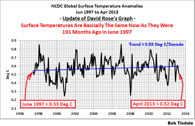
In his RMS article, Kevin Trenberth also conveniently overlooked the fact that the discussions about the warming halt are now for a time period of about 16 years, not 10 years—ever since David Rose’s DailyMail article titled “Global warming stopped 16 years ago, reveals Met Office report quietly released… and here is the chart to prove it”. In my response to Trenberth’s article, I updated David Rose’s graph, noting that surface temperatures in April 2013 were basically the same as they were in June 1997. We’ll use June 1997 as the start month for the running 17-year trends. The period is now 204-months long. The following graph is similar to the one above, except that it’s presenting running trends for 204-month periods.

Figure 7 – 204-Month Linear Trends
The last time global surface temperatures warmed at this low a rate for a 204-month period was the late 1970s, or about 1980. Also note that the sharp decline is similar to the drop in the 1940s, and, again, as you’ll recall, global surface temperatures remained relatively flat from the mid-1940s to the mid-1970s.
The most widely used metric of global warming—global surface temperatures—indicates that the rate of global warming has slowed drastically and that the duration of the halt in global warming is unusual during a period when global surface temperatures are allegedly being warmed from the hypothetical impacts of manmade greenhouse gases.
A NOTE ABOUT THE RUNNING-TREND GRAPHS
There is very little difference in the end point trends of 13+ year and 16+ year running trends if HADCRUT4 or NCDC or GISS data are used. The major difference in the graphs is with the HADCRUT4 data and it can be seen in a graph of the 13+ year trends. I suspect this is caused by the updates to the HADSST3 data that have not been applied to the ERSST.v3b sea surface temperature data used by GISS and NCDC.
COMPARISONS
The GISS, HADCRUT4 and NCDC global surface temperature anomalies and the RSS and UAH lower troposphere temperature anomalies are compared in the next three time-series graphs. Figure 8 compares the five global temperature anomaly products starting in 1979. Again, due to the timing of this post, the HADCRUT4 and NCDC data lag the UAH, RSS and GISS products by a month. The graph also includes the linear trends. Because the three surface temperature datasets share common source data, (GISS and NCDC also use the same sea surface temperature data) it should come as no surprise that they are so similar. For those wanting a closer look at the more recent wiggles and trends, Figure 9 starts in 1998, which was the start year used by von Storch et al (2013) Can climate models explain the recent stagnation in global warming? They, of course found that the CMIP3 (IPCC AR4) and CMIP5 (IPCC AR5) models could NOT explain the recent halt in warming.
Figure 10 starts in 2001, which was the year Kevin Trenberth chose for the start of the warming halt in his RMS article Has Global Warming Stalled?
Because the suppliers all use different base years for calculating anomalies, I’ve referenced them to a common 30-year period: 1981 to 2010. Referring to their discussion under FAQ 9 here, according to NOAA:
This period is used in order to comply with a recommended World Meteorological Organization (WMO) Policy, which suggests using the latest decade for the 30-year average.

Figure 8 – Comparison Starting in 1979
###########

Figure 9 – Comparison Starting in 1998
###########

Figure 10 – Comparison Starting in 2001
AVERAGE
Figure 11 presents the average of the GISS, HADCRUT and NCDC land plus sea surface temperature anomaly products and the average of the RSS and UAH lower troposphere temperature data. Again because the HADCRUT4 and NCDC data lag one month in this update, the most current average only includes the GISS products.

Figure 11 – Average of Global Land+Sea Surface Temperature Anomaly Products
The flatness of the data since 2001 is very obvious, as is the fact that surface temperatures have rarely risen above those created by the 1997/98 El Niño in the surface temperature data. There is a very simple reason for this: the 1997/98 El Niño released enough sunlight-created warm water from beneath the surface of the tropical Pacific to permanently raise the temperature of about 66% of the surface of the global oceans by almost 0.2 deg C. Sea surface temperatures for that portion of the global oceans remained relatively flat until the El Niño of 2009/10, when the surface temperatures of the portion of the global oceans shifted slightly higher again. Prior to that, it was the 1986/87/88 El Niño that caused surface temperatures to shift upwards. If these naturally occurring upward shifts in surface temperatures are new to you, please see the illustrated essay “The Manmade Global Warming Challenge” (42mb) for an introduction.
MONTHLY SEA SURFACE TEMPERATURE UPDATE
The most recent sea surface temperature update can be found here. The satellite-enhanced sea surface temperature data (Reynolds OI.2) are presented in global, hemispheric and ocean-basin bases.
TABLE OF CONTENTS OF UPCOMING BOOK
I linked a copy to the post here of the Table of Contents for my upcoming book about global warming, climate change and skepticism. Please take a look to see if there are topics I’ve missed that you believe should be covered. I’ve already removed the introductory chapters for climate models from Section 1, and provided a separate section for those model discussions. Section 1 now only includes the chapters that introduce global warming and climate change topics. (Thanks, Gary.) Please also post any comments you have on that thread at my blog. Otherwise, I might miss them.
Thanks
Bob Tisdale
Henry P,
There is no measurable AGW. That isn’t a hypothesis, that is reality.
Simon says:
June 24, 2014 at 1:02 am
“I will concede though that the rate of warming has slowed in the atmosphere/on land, but if the scientists are to be believed and most of the warming has gone into the oceans, then the air will soon reflect that energy in our temp readings.”
The air will never “reflect that energy in our temp readings”. By the 2nd Law of Thermodynamics, the oceans cannot heat the atmosphere beyond their temperature differential. So, in the worst possible case, that energy can only go into the atmosphere to the point where the atmospheric temperature rise is the same as the ocean temperature rise. After that, they can only release the energy to maintain that atmospheric temperature level at the same rate as the atmosphere loses it to space.
The heat capacity of the oceans is vast, and the increase in temperature of the oceans, even in the highly unlikely event of the immaculate convection of CO2 induced heat to the depths according to the narrative, is utterly negligible. Hundredths of a degree. We are not worried about a hundredths of a degree rise in atmospheric temperatures. You should not be worried about a hundredths of a degree rise in atmospheric temperatures.
dbstealey
There is no measurable AGW. That isn’t a hypothesis, that is reality.
———————————
Ha ha. Well someone better tell these people
http://opr.ca.gov/s_listoforganizations.php
Simon:
re your post at June 24, 2014 at 10:12 pm.
There is no need to tell those organisations that there is no measurable AGW because they know.
Anybody who wants to know how the Executives of those organisations were deliberately usurped can obtain the shocking information – which names names – in this paper by Lindzen; it is is a shocking and entertaining read
http://www.globalresearch.ca/climate-science-is-it-currently-designed-to-answer-questions/16330
Richard
@db stealey
Both of us already agree on AGW, ie. that there is none. I think you did get what I was asking about.
@Bart, db stealey
I’d be interested to hear from you whether you agree with me that the climate is changing,
naturally, i.e. we are cooling
http://www.woodfortrees.org/plot/hadcrut4gl/from:1987/to:2015/plot/hadcrut4gl/from:2002/to:2015/trend/plot/hadcrut3gl/from:1987/to:2015/plot/hadcrut3gl/from:2002/to:2015/trend/plot/rss/from:1987/to:2015/plot/rss/from:2002/to:2015/trend/plot/hadsst2gl/from:1987/to:2015/plot/hadsst2gl/from:2002/to:2015/trend/plot/hadcrut4gl/from:1987/to:2002/trend/plot/hadcrut3gl/from:1987/to:2002/trend/plot/hadsst2gl/from:1987/to:2002/trend/plot/rss/from:1987/to:2002/trend
Note that my results show current speed of cooling at -0.014K/annum (since 2000)
Sorry, I see now that I had missed an update on my means table.
We are currently cooling at a rate of -0.015K/annum, average since 2000.
That is not worrying anyone?
richardscourtney says:
June 24, 2014 at 1:11 pm
Troll posting as Phil.:
I see that at June 24, 2014 at 12:17 pm you acknowledge your misrepresentation of the “fallback” issue has failed because you attempt to again move the goal posts. Now you try to argue about the ‘hotspot’ instead of stratospheric cooling.
I’m undecided on whether you don’t read the posts you respond to or you’re just a liar.
As I clearly stated, instead of replying to your misrepresentations of Stealey’s original statements I returned to the original and made the same rebuttals as I had previously. In addition I responded to his first point about the ‘hotspot’ itself.
The IPCC AR4 said the tropospheric hot spot was an effect of warming by GHGs.
You say it is an effect of warming from any cause.
No the science says that it can be caused by any source of warming, due to the increased water vapor present as a result of the warming. I quoted Dr Roy Spencer, a frequent contributor here, who made that point in a posting here but could have referred to many others.
THE HOTSPOT HAS NOT HAPPENED.
If the IPCC AR4 is right that means there has been no global warming from GHGs.
And
If you are right that means there has been no global warming from any cause.
In either case your retreat from your fallacious misrepresentation of the ‘fallback issue’ asserts that there is no AGW.
There is no ‘retreat’ since I haven’t changed my position, either read the post or stop lying about it.
Troll posting as Phil.:
Your problem is that I do read the falsehoods and the stupidities you write, and I refute them.
You have moved the goal posts to the tropospheric hotspot from your original and wrong point about stratospheric cooling. Everybody can see that “retreat”, and your bluster does not – and cannot – hide it.
The amusing point is that your new assertion refutes your claims of AGW!
As I said
Richard
Friends:
There may be some who have been misled by the troll posting as “Phil.”.
The nature of the tropospheric hotspot is described in Chapter 9 of the IPCC AR4 WG1 Report and can be seen here
https://www.ipcc-wg1.unibe.ch/publications/wg1-ar4/ar4-wg1-chapter9.pdf
Figure 9.1 is on page 675 of that document.
The Figure is titled
The hotspot is the big, red blob which only exists in (c) wellmixed greenhouse gases, and in (f) the sum of all forcings (which includes the effect of wellmixed greenhouse gases).
It represents a rate of warming at altitude in the tropics which is 2x to 3x the rate of warming at the surface. And it occurs because the model assumes the water vapour feedback (WVF) increases the warming effect of other greenhouse gases.
Richard
Simon,
Richard beat me to it, I was going to post that Lindzen link.
Your constant appeals to authority are tedious. Appeal to Authority is a fallacy that only works with people who do not think, like you.
Those ‘authorities’ are corrupted, as Prof. Lindzen makes clear. Read in particular Section 2.
The only credible climate Authority at this point is Planet Earth, which is flatly contradicting every ‘authority’ you posted — they are all wrong.
You never answer questions, cementing your role as a troll. But you could try to answer just one simple question:
Who should we believe? Your ‘authorities’?
Or Planet Earth?
Because they cannot both be right.
Either start having a discussion without constantly moving the goal posts, or setting up strawmen, or refusing to respond to questions, or your comments will be consigned to the bit bucket for multiple site rule infractions.
Finally, there are no measurements of AGW. Instead of saying, ‘haha’, post a testable, verifiable measurement showing AGW. Do not bother with anything showing general global warming, we already know natural global warming is happening.
That is a challenge to you. Like all other challenges, you know you will fail, so you will change the subject, or ignore it, or exhibit some other troll behavior. See the paragraph above, and don’t complain when it happens.
HenryP says:
June 24, 2014 at 1:12 pm
phil. says
http://wattsupwiththat.com/2014/06/18/may-2014-global-surface-landocean-and-lower-troposphere-temperature-anomaly-update/#comment-1668561
Henry says
I am puzzled that I would have to explain here high school stuff about throwing a ball and what curve it goes. Obviously it is parabolic and excell shows you the equation and the correlation if you punch in the data points. 4 points is all I need, as long as I do not go outside (to predict)
I asked for clarification because you also referred to it as a binomial, which in general quadratic isn’t.
Using such a small number of points guarantees a strong correlation, it doesn’t really tell you much.
A quadratic has three parameters and so needs three points to define it. in your case you appear to be using overlapping data, how are you dealing with that?
richardscourtney 4:34am: “And (hotspot) occurs because the model assumes the water vapour feedback…”
Thru inspection of model results compared to observations of top post anomaly, the GC models have not proven reliable forecasters of Tmean anomaly so far on out of sample data. That GCMs show a “hotspot” – does not invalidate the 1st principle physics of IR active gas in an atmosphere & only confirm the system modeling is suspect. The “hotspot” is a symptom of attempts modeling huge complex chaotic system not basic IR active gas science long established by replicable lab test & reasoned analysis.
******
dbstealey 5:02am: “Appeal to Authority is a fallacy..”
When the appeal is properly made to a generally accepted authority it is not a fallacy. Proof is in teaching methods work out fairly well using generally accepted text books properly chosen based on test & original cites. If the appeal results in simple assertion or is circular, then the appeal can be fallacious.
“The only credible climate Authority at this point is Planet Earth…Who should we believe?…That is a challenge.”
To answer your challenge, believe those that can run a control experiment of a real & duplicate Planet Earth system without humans adding IR active gas in order to determine if AGW exists by measurable anomaly in the two system’s global surface Tmean.
Absent that, I predict blogging will drift into and out of proper appeal to authority & attacks on the basic IR active gas science for shock and/or entertainment value. At least until reduced CIs become more informative on system surface Tmean response to single parameter perturbation.
richardscourtney says:
June 25, 2014 at 4:34 am
Friends:
There may be some who have been misled by the troll posting as “richardscourtney”.
“The nature of the tropospheric hotspot is described in Chapter 9 of the IPCC AR4 WG1 Report and can be seen here
https://www.ipcc-wg1.unibe.ch/publications/wg1-ar4/ar4-wg1-chapter9.pdf
Figure 9.1 is on page 675 of that document.
The Figure is titled
Zonal mean atmospheric temperature change from 1890 to 1999 (°C per century) as simulated by the PCM model from
(a) solar forcing,
(b) volcanoes,
(c) wellmixed greenhouse gases,
(d) tropospheric and stratospheric ozone changes,
(e) direct sulphate aerosol forcing
and
(f) the sum of all forcings.
Plot is from 1,000 hPa to 10 hPa (shown on left scale) and from 0 km to 30 km (shown on right). See Appendix 9.C for additional information. Based on Santer et al. (2003a).
The hotspot is the big, red blob which only exists in (c) wellmixed greenhouse gases, and in (f) the sum of all forcings (which includes the effect of wellmixed greenhouse gases).
It represents a rate of warming at altitude in the tropics which is 2x to 3x the rate of warming at the surface. And it occurs because the model assumes the water vapour feedback (WVF) increases the warming effect of other greenhouse gases.”
Since my earlier post from June 24, 2014 at 12:17 pm has apparently been deleted I’ll refer you to Spencer’s post again. (Mods perhaps you could restore it or if not delete Courtney’s misrepresentation of it? richardscourtney says: June 24, 2014 at 1:11 pm)
Talking specifically about that figure Spencer says:
“But all the figure demonstrates is that the warming influence of GHGs is stronger than that from a couple of other known external forcing mechanisms, specifically a very small increase in the sun’s output, and a change in ozone. It says absolutely nothing about the possibility that warming might have been simply part of a natural, internal fluctuation (cycle, if you wish) in the climate system.”
“But the hotspot is not a unique signature of manmade greenhouse gases. It simply reflects anomalous heating of the troposphere — no matter what its source. Anomalous heating gets spread throughout the depth of the troposphere by convection, and greater temperature rise in the upper troposphere than in the lower troposphere is because of latent heat release (rainfall formation) there.”
“The heating in the upper troposphere is not from water vapor at that level, but rising from below condensing and releasing latent heat. It is BECAUSE the specific humidity is limited at 200 mb that water ascending to the level must be precipitated out. Also, remember the heat capacity of air at 200 mb is only 20% of that at 1000 mb (less air to heat), which helps amplify a temperature rise.”
http://wattsupwiththat.com/2009/10/11/spotting-the-agw-fingerprint/
Troll posting as Phil.:
I am writing to draw attention to your incredibly funny post at June 25, 2014 at 6:18 am. It is Pythonesque.
It quotes my quotation of what the IPCC AR4 says and repeats your silly assertion concerning your retreat argument about the hotspot.
I again point out that you have switched to the hotspot because you failed in your attempts to misrepresent about stratospheric cooling being a “fallback”. And, importantly, your retreat position refutes your claims of AGW!
As I said
The IPCC AR4 said the tropospheric hot spot was an effect of warming by GHGs.
You say it is an effect of warming from any cause and cite Spencer in support of that.
THE HOTSPOT HAS NOT HAPPENED.
If the IPCC AR4 is right that means there has been no global warming from GHGs.
And
If you are right that means there has been no global warming from any cause.
In either case your retreat from your fallacious misrepresentation of the ‘fallback issue’ asserts that there is no AGW.
I agree that there is no discernible AGW.
Richard
richardscourtney says:
June 25, 2014 at 8:26 am
Troll posting as Phil.:
I am writing to draw attention to your incredibly funny post at June 25, 2014 at 6:18 am. It is Pythonesque.
I’m glad it amuses you.
It quotes my quotation of what the IPCC AR4 says and repeats your silly assertion concerning your retreat argument about the hotspot.
No it does not, it links to Roy Spencer’s WUWT post concerning the ‘hotspot’, are you saying Roy’s post is silly? Or like before you didn’t really read it and failed to notice that it was his? The only reason I repeated it is that the earlier post which referred to it was deleted, more of Stealey’s chicanery no doubt.
I again point out that you have switched to the hotspot because you failed in your attempts to misrepresent about stratospheric cooling being a “fallback”. And, importantly, your retreat position refutes your claims of AGW!
No, I’ve proved the point about Stealey’s errors, I see no point in continuing to debate them with a troll such as yourself.
As I said
The IPCC AR4 said the tropospheric hot spot was an effect of warming by GHGs.
You say it is an effect of warming from any cause and cite Spencer in support of that.
THE HOTSPOT HAS NOT HAPPENED.
If the IPCC AR4 is right that means there has been no global warming from GHGs.
And
If you are right that means there has been no global warming from any cause.
In either case your retreat from your fallacious misrepresentation of the ‘fallback issue’ asserts that there is no AGW.
Firstly, there is no ‘retreat’, secondly if you understood Spencer’s argument you would realize that it doesn’t mean that at all.
Phil. says
I asked for clarification because you also referred to it as a binomial, which in general quadratic isn’t.
Using such a small number of points guarantees a strong correlation, it doesn’t really tell you much.
A quadratic has three parameters and so needs three points to define it. in your case you appear to be using overlapping data, how are you dealing with that?
Henry says
Even for a linear function, like in photometry, you need at least 3 points. If there is a bend, like in AAS (e.g. for tin) you need at least 4 points.
That is my point. You only need 4 measuring points to see what the function looks like, and to define it mathematically.
In Excell they give you the option of a polynomial fit of various orders. I used the 2nd order here. Generally speaking (I am not sure in USA?) a polynomial of the second order, i.e a quadratic function, is also referred to as a bi-nomial. Perhaps you learned something else?
The overlap is irrelevant. I measured the average speed of warming over 4 periods of time, i.e. the average change in K/annum from the average of that whole period. Once you have those 4 points (from the linear regressions of all the results in each of those 54 stations) you can set that [average of 54 stations] out against time to observe acceleration/deceleration (K/yr square)
It is really quite simple.
Troll posting as Phil.:
I see that in your post at June 25, 2014 at 9:28 am you again attempt your favourite trolling tactic of disingenuous distraction. How many times have you done it this thread now; four, isn’t it?
You pretend that I am disputing with Spencer. No! I am laughing at you.
You made an assertion which – if accepted – demonstrates there has been no global warming from any cause. You chose who and what to cite in support of your assertion.
The reason you made the assertion was as a smokescreen for you having been shown to be wrong about use of stratospheric warming as a warmunist “fallback” position.
Now you try to start an argument about what you assert Spencer wrote and try to use the argument as a smokescreen for your assertion being shown to indicate there has been no discernible global warming from any cause.
So, I see no reason to argue about what you claim Spencer said. I repeat what I said as conclusion in my post you purport to be answering,
I agree that there is no discernible AGW.
Richard
Trick:
re your post at June 25, 2014 at 5:52 am.
The climate models all fail as devices to predict future climate. Live with it.
Richard
richardscourtney 10:11am: “..climate models all fail Live with it.”
Agreed for GCMs in bulk & I am interested to watch for continuous improvement in those GCMs out of sample. More basic Callendar 1938 surface Tmean anomaly predictions have stood the test of time to reasonable approx. CI out of sample to top post instrumental data measured over centuries, rounded.
Trick says:
If the appeal results in simple assertion or is circular, then the appeal can be fallacious.
Thank you for that. Simple assertions are the basis for those groups’ position. All it takes are a few activists on the Board — just one or two is sufficient — and the entire organization can be turned to a particular narrative. That is what has happened, as documented by Prof. Lindzen.
To date there is no testable, merasurable scientific evidence quantifying the putative fraction of a degree of temperature change due to human CO2 emissions. Thus, the position of those groups is nothing more than a baseless assertion. Therefore, it is a fallacy to appeal to their ‘authority’, particularly since those ‘authorities’ are contradicted by the only real Authority: Planet Earth.
HenryP says:
June 25, 2014 at 9:51 am
Even for a linear function, like in photometry, you need at least 3 points. If there is a bend, like in AAS (e.g. for tin) you need at least 4 points.
That is my point. You only need 4 measuring points to see what the function looks like, and to define it mathematically.
But if you use the minimum the goodness of fit is meaningless.
In Excell they give you the option of a polynomial fit of various orders. I used the 2nd order here. Generally speaking (I am not sure in USA?) a polynomial of the second order, i.e a quadratic function, is also referred to as a bi-nomial. Perhaps you learned something else?
A binomial is the sum of two monomials, therefore only two terms, a quadratic has three, that’s why I asked.
The overlap is irrelevant. I measured the average speed of warming over 4 periods of time, i.e. the average change in K/annum from the average of that whole period. Once you have those 4 points (from the linear regressions of all the results in each of those 54 stations) you can set that [average of 54 stations] out against time to observe acceleration/deceleration (K/yr square)
It is really quite simple.
A strange way to do it, why not do it per decade with no overlap?
[snip. Site Policy: Internet phantoms who have… no name… get no respect here. If you think your opinion or idea is important, elevate your status by being open and honest. People that use their real name get more respect than phantoms with handles. The idea of the blog is to learn and discuss. Constantly changing the subject, and a refusal to discuss subjects that are raised but then may lead to an uncomfortable conclusion for one party are not acceptable behavior. Discussion requires an honest give and take, no mater where it leads. ~mod.]
Simon:
Yet again you ignore what you are told.
At June 25, 2014 at 11:54 am you claim I think you are merely “silly” and “deluded”.
No! I made it very clear and in very plain language that I consider you with disdain.
My contempt is much, much more than would be the case if I thought you were merely “silly” and “deluded”.
You are clearly a troll pretending complete stupidity as a method to publish misleading nonsense on the world’s most successful science blog. You may be obtaining remuneration for doing this or merely doing it from malign intent. Either way, interacting with you has similar emotion to removing something unpleasant from the instep of a shoe.
I hope you have now grasped what I really think of you.
Richard
Troll posting as Phil.:
I have read your post at June 25, 2014 at 12:28 pm.
As I understand it,
1.
You do not dispute that your argument about the hotspot asserts there has been no global warming from any cause.
2.
You want to argue about what you claim Spencer said because that will smokescreen the fact of your argument about the hotspot asserting there has been no global warming from any cause.
3.
You have abandoned your original – and very silly – assertion that stratospheric cooling was not used as a “fallback” when the hotspot failed to occur.
Do you agree that is a fair and accurate summary?
Richard
@Phil.
with linear regression, the more points you have (i.e. the actual average yearly temperatures measured at the station), the higher the accuracy. For the shortest period (from 2000) the number of measuring points is actually barely enough.
Nevertheless, the last point [for minima] is still accurate – must be-
last 40 years (from 1974) 0.004K/annum
last 34 years (from 1980) 0.007K/annum
last 24 years (from 1990) 0.004K/annum
last 14 years (from 2000) -0.009K/annum
as together it gives me a perfect parabolic function with correlation coefficient:1.000
So, there is no room for any AGW [for minima]
Unless the AGW follows a perfect parabolic curve the same as the natural one?
I think we are all agreed here that there is no discernible AGW
[except simon but he has no results of his own so his word does not count – I told you all that you are wasting your time with him.]