Guest essay by Joe Born
In a recent post Christopher Monckton identified me as a proponent of the following proposition: The observed decay of bomb-generated atmospheric-carbon-14 concentration does not tell us how fast elevated atmospheric carbon-dioxide levels would subside if we discontinued the elevated emissions that are causing them. He was entirely justified in doing so; I had gone out of my way to bring that argument to his attention.
But I was merely passing along an argument to which a previous WUWT post had alerted me, and the truth is that I’m not at all sure what the answer is. Moreover, semantic issues diverted the ensuing discussion from what Lord Monckton probably intended to elicit. So, at least in my view, we failed to join issue.
In this post I will attempt to remedy that failure by explaining the weakness that afflicts the position attributed (again, understandably) to me. I hasten to add that I don’t profess to have the answer, so be forewarned that no conclusion lies at the end of this post. But I do hope to make clearer where at least this layman thinks the real questions lie.

To start off, let’s review the argument I made, which is that the atmospheric-carbon-dioxide turnover time is what determined how long the post-bomb-test excess-carbon-14 level took to decay. That argument was based on the “bathtub” model, which Fig. 1 depicts. The rate at which the quantity <i>m</i> of water the tub contains changes is equal to the difference between the respective rates <i>e</i> (emissions) and <i>u</i> (uptake) at which water enters from a faucet and leaves through a drain:

The same thing can, <i>mutatis mutandis</i>, be said of contaminants (read carbon-14) in the water. But in the case of well-mixed contaminants one of the <i>mutanda</i> is that the rate at which the contaminants leave is dictated by the rate at which water leaves:

where 

Consequently, if the water quantity increases for an interval during which <i>e</i> exceeds <i>u</i>, it will thereafter remain elevated if the emissions rate <i>e</i> then falls no lower than the drain rate <i>u</i>. If a dose of contaminants is added to the water, though, the resultant contaminant amount falls, even when there’s no difference between <i>u</i> and <i>e</i>, in accordance with the <i>turnover</i> rate, i.e., with the ratio of <i>u</i> to <i>m</i>. So, to the extent that this model reflects reality’s relevant aspects, we can conclude that the rate at which the carbon-14 concentration decays tells us nothing about what happens when total-CO2 emissions return to a “normal” level.
But among the foregoing model’s deficiencies is that it says nothing about a possible dependence of overall drain rate <i>u</i> on the water quantity <i>m</i>, whereas we may expect biosphere uptake (and emissions) to respond to the atmosphere’s carbon-dioxide content. Nor does it deal with the possibility that after contamination has flowed out the drain it will be recycled through the faucet. In contrast, the biosphere no doubt returns to the atmosphere at least some of the carbon-14 it has previously taken from it.

A model that takes such factors into account could support a conclusion different from the one to which the bathtub led us. Consistently with my last post’s approach, Fig. 2 uses interconnected pressure vessels to represent one such model. In this case there are only two vessels, the left one representing the atmosphere and the right one representing carbon sinks such as the ocean and the biosphere.
The vessels contain respective quantities 


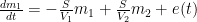
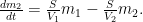
Those equations tell us that the carbon quantity 
![m_1(t) = \left[ \frac{V_1}{V_1+V_2}+\frac{V_2}{V_1+V_2} \exp\left(-\frac{V_1+V_2}{V_1V_2}St \right)\right] m_0 ,](https://s0.wp.com/latex.php?latex=m_1%28t%29+%3D+%5Cleft%5B+%5Cfrac%7BV_1%7D%7BV_1%2BV_2%7D%2B%5Cfrac%7BV_2%7D%7BV_1%2BV_2%7D+%5Cexp%5Cleft%28-%5Cfrac%7BV_1%2BV_2%7D%7BV_1V_2%7DSt+%5Cright%29%5Cright%5D+m_0+%2C+&bg=ffffff&fg=000&s=0&c=20201002)
which the substitutions 

Note that in the Fig. 2 system any constituent of the gas would be exchanged between vessels in accordance with the partial-pressure difference of that constituent alone, as if it were the only component the vessels contained. By thus constraining the flow from (and to) the first, atmosphere-representing vessel, this model supports the conclusion that the overall-carbon-dioxide quantity would, contrary to my previous argument, decay just as the excess, bomb-caused quantity of atmospheric carbon-14 did.

Could providing more than one sink enable us to escape that conclusion? Not necessarily. Consider the more-complex system that Fig. 3 depicts. Just as the system that my previous post described, this one can embody the TAR Bern-model parameters. As that post indicated, describing such a system requires a fourth-order linear differential equation. So that system does have more degrees of freedom in its initial conditions and can therefore exhibit a wider range of responses.
But it still constrains the flow among its four vessels linearly in accordance with partial pressures, just as the Fig. 2 system does. From complete equilibrium, therefore, its behavior for any constituent is the same as for any other constituent as well as for the contents as a whole. In other words, this model, too, seems to support the notion that the bomb-test results do indeed tell us how long excess carbon dioxide will remain if we stop taking advantage of fossil fuels.
In a sense, though, the models of Figs. 2 and 3 beg the question; they use the same uptake- and emissions-process-representing
So one question is how significant that difference is in the present context. I don’t have the answer, although my guess is, not very. But readers attempting to answer that question could do worse than start by referring to a previous WUWT post by Ferdinand Engelbeen.

Another way in which carbon-14 differs from the other two carbon isotopes is that it’s unstable. So, if the Fig. 3 model is adequate for carbon-12 or -13, a different model, which Fig. 4 depicts, would have to be used for carbon-14 if its radioactive decay is significant. That diagram differs from Fig. 3 in that it includes a flow 
To the extent that those different models produce different responses, using bomb-test data to predict the total carbon content’s behavior is problematic. But the Engelbeen post mentioned above seems to say that even deep-ocean residence times tend to be only a minor fraction of carbon-14’s half-life: this factor’s impact may be small.
A possibly more-significant factor is that the carbon cycle is undoubtedly non-linear, whereas the conclusions we tentatively drew from the models above depend greatly on their linearity. Before I reach that issue, though, I should point out an aspect of the Bern model that was not relevant to my previous post. The Bern equations I set forth in my last post were indeed linear. But that does not mean that their authors meant to say that the carbon cycle itself is. Although for the sake of simplicity I’ve discussed the models’ physical quantities as though they represented, e.g., the entire mass of carbon in a reservoir, their authors no doubt intended their (linear) models’ quantities to represent only the differences from some base, pre-industrial values. Presumably the purpose was to limit their range enough that the corresponding real-world behavior would approximate linearity.
But such linearization compromises the conclusions to which the models of Figs. 2 and 3 led us. A linear system is distinguished by the fact that its response to a composite stimulus always equals the sum of its individual responses to the stimulus’s various constituents; if the stimulus equals the sum of a step and a sine wave, for example, the system’s response to that stimulus will equal the sum of what its respective responses would have been to separate applications of the step and the sine wave. And this “superposition” property was central to drawing the conclusions we did from those models: the response to a large stimulus is proportionately the same as the response to a small one.

To appreciate this, consider Fig. 5, which depicts scaled values of the Fig. 2 model’s left-vessel total-carbon and carbon-14 contents. Initially, the system is at equilibrium, with zero outside emissions 


At time t = 5, a bolus of carbon-14 appears in the (atmosphere-representing) left vessel. Compared with the total carbon content, the added quantity is tiny, but it is large enough to double the small existing carbon-14 content. As the distance between the red dotted vertical lines shows, the resultant increase in carbon-14 content decays toward its new equilibrium value with a time constant of just about seven years. (I’ve assumed that the processes greatly favor the sink-representing right vessel—i.e., that its “volume” is much greater than the left vessel’s—so that the new equilibrium value is not much greater than the original.)
Now consider what happens at t = 45, when the left vessel’s total-carbon quantity suddenly increases. Although the two quantities are scaled to their respective initial values, this total-carbon increase is orders of magnitude greater than the t = 5 carbon-14 increase. Yet, as the black dotted vertical lines show, the decay of the left vessel’s total-carbon content proceeds just as fast proportionately as the much-smaller carbon-14 content did. As was observed above, this could tempt one to conclude that the carbon-14 decay we’ve observed in the real world tells us how fast the atmosphere would respond to our discontinuing fossil-fuel use.
![clip_image009[1]](http://wattsupwiththat.files.wordpress.com/2013/12/clip_image0091.png?quality=75 "clip_image009[1]")
But now consider what can happen if we relax the linearity assumption. Specifically, let’s say that the Fig. 2 model’s proportionality “constant”

In that plot, the red lines show that the carbon-14 decay occurs just as fast as in the previous plot, the carbon-14 content falling to exp(-1) above its new equilibrium value in around seven years. But the much-larger total-carbon increase brings the system into a lower-efficiency range, so that quantity subsides at a more-leisurely pace, taking over forty years. If such results are any indication, bomb-test results are a poor predictor of how long total-carbon content will settle.
Now permit me a digression in which I attempt to forestall pointless discussion of precisely what the quantities are that the graphs show. I believe the exposition is clearest if it is directed, as in Figs. 5 and 6, to ratios that carbon 14 and total carbon bear to their own initial values. But it appears customary to express the carbon-14 content instead in terms of its ratio to total carbon content. This means that, since total carbon has been increasing, the numbers commonly used in carbon-14 discussions could fall below the pre-bomb values, even though total carbon-14 has in fact increased.
For the sake of those to whom that issue looms large, I have attached Fig. 7 to illustrate how the values for carbon-14 itself could differ from those of its ratio to total carbon in a situation in which new (carbon-14-depleted) carbon is continually injected into the atmosphere.

But that’s a detail. More important is the issue that Fig. 6 raises.
Now, I “cooked” Fig. 6’s numbers to emphasize the point that nonlinearity can undermine conclusions based on linear models. Specifically, Fig. 6 depicts the results of making the flows proportional only to the fifth root of the carbon content.
But non-linearity must have some effect. How much? I don’t know. Together with the differences in behavior between carbon-14 and its stable siblings, though, it is among the considerations to take into account in assessing how informative the bomb-test data are.
As I warned at the top of the post, this post draws no conclusions from these considerations. But maybe the foregoing analysis will prompt knowledgeable readers’ comments that help narrow the issues.
rgb at duke, thank you for the link to the fluctuation-dissipation theorem.
De nada. Not enough people outside of physics seem aware of it, or seem aware that it is relevant to the climate. A thorough analysis of the noise in the climate system would actually teach us a lot about the underlying linear response coefficients of the many coupled processes that drive it. Roy Spencer effectively used it (but not by name) in work he talks about in his book — analyzing the lifetime of persistent fluctuations to try to determine the sign of certain feedbacks, IIRC. I’ve tried to encourage him to do more of the same, as I think it is a gold mine of information, especially about the rapidly fluctuating water cycle.
rgb
Ferdinand, You are drowning in a sea of detail (if not comments), one of your own making. Step back and look at the big picture. Hoser and phlogiston are bang on. Their points lead to the same conclusion – Monckton’s thesis on CO2.
_Jim says:
December 12, 2013 at 7:36 am
“Michael, that is just plain nuts, but you don’t know that.”
Nice to see you’re still obsessed with following me Jim. I must be doing something right, unlike you who can only write ad hominem attacks. Sorry we had to bust your Romney bubble, but you needed to be taught a lesson you will never forget. Besides, Romney wouldn’t have hesitated in attacking Syria and starting WW3. Actually the democrats are learning a valuable lesson from their devotion to Obama as well these days. Win Win. The divide and conker strategy, Red Team vs Blue Team, is so yesterday.
Joe Born says:
December 12, 2013 at 9:08 am
The problem is in the following:
Now we’ll tell the same story, but this time we’re talking total carbon, of which the content has been 1000M for eons. It loses 100M every year to the Arctic Ocean but receives 100M back every year from the Southern Ocean, so its content remains the same. Now another 1000M is suddenly added, doubling the atmospheric content to 2000M, but the Arctic Ocean responds by taking 200M, while the Southern Ocean still is returning only 100M, so the total-carbon content decays by 100M.
The circulation of 14C was 100M into the oceans, 90M out, 10M production in the atmosphere.
A doubling of 14C in the atmosphere gives 200M into the oceans, 90 M out, 10 M production, a loss of 100M 14C.
So far so good.
The circulation of 12C was 100M into the oceans, 100M out.
A doubling of 12C in the atmosphere doesn’t give 200M into the oceans, but only 110M and 90M out, a loss of 20M 12C.
Why the difference?
The 100M 14C is transported by 100M 12C in and out. That is a temperature dependent process: the high temperatures at the upwelling places give a continuous stream of CO2 in the atmosphere and the low temperatures near the poles give a permanent sink of CO2.
The 100M 14C in and out follows the same rules as the 12C transport in/out for the same temperature difference and as the extra mass of 14C is negligible, there is no change in mass flow of 12C.
If you add 100M extra 12C, then you invoke a different process.
Assuming that the temperature of the seawater didn’t change, the pCO2(aq) didn’t change at the upwelling and downwelling places. But the pCO2 of the atmosphere doubled.
The most extreme pCO2 levels found in the oceans were 150 μatm at the sink places and 750 μatm at the source places. That made a more or less balanced in/outflux at ~40 GtC/year for an atmosphere at pre-industrial 290 μatm.
For the sink places:
100M / (290-150) μatm = 0.71M / μatm
For the source places:
100M / (750-290) μatm = 0.22M / μatm
Now we increase the 290 μatm in the atmosphere to 580 μatm:
For the sink places:
100M * (580-150) / (290-150) = 307M
For the source places:
100M * (750-580) / (750-290) = 37M
The net increase in sink rate in this case increased from a balanced zero change to 107 GtC/year sink rate. Compared to the balanced flux, the sink rate is 2.5 times higher. For the sink places, a doubling in the atmosphere gives a tripling in output rate. For the source places, a doubling in the atmosphere gives an almost 3-fold decrease in input.
As you can see, there is not the slightest connection with the 14C decay rate which is based on an unchanged throughput, but a huge change in concentrations, while the 12C decay rate is based on huge changes in in/out fluxes, but no change in concentrations.
Several caveats: the calculation is for the most extreme differences in a small area of the oceans, not direct translateable to the full oceans surface. For that purpose one need all pCO2 differences in all areas and where the direct sink/source areas from the deep oceans are…
The real, measured net sink rate is about 2.15 ppmv/year for an increase of 110 ppmv in the atmosphere above equilibrium (~290 ppmv) at the current temperature. Or an e-fold decay rate of 110/2.15 = ~50 years.
Hoser,
“For one thing, it becomes pretty clear the increase in atmospheric CO2 cannot possibly be due to anthropogenic CO2. The CO2 quantity changes simply don’t match what humans have produced given the amount of CO2 we have produced each year from the late 1700s and how much would be left Y years after emission.”
Can you give details please ?
stas peterson: “There ar eat least two missing “drain effects” on oceanic CO2 that are not accounted for. There is a drain rate due to the formation of limestone, and the drain rate due to algal formation of one type the most common type of Carbon by life, in the form of algal photosynthesis. Which in turn becomes plant and animal mass,and on death da significant proportion descends ot the abyssal depths.”
Exactly so. I omitted those and other effects I thought of because they would have unduly complicated an already long post. And, for present purposes, they were not relevant; in contrast to the beta-decay leak, those additional effects do not treat the different isotopes much differently from each other.
DocMartyn says:
December 12, 2013 at 8:39 am
We have a language that has defined terms. Top and bottom have actual meanings, as do the phrases ‘deep water’ and ‘surface water’. Why do you want to destroy the accepted convention of what words actually mean? The interface between the atmosphere and the oceans is at the surface; period.
Doc, you are sometimes a difficult person to discuss with. Of course the deep oceans connect with the atmsophere via a surface layer. But that surface layer is not the whole “mixed layer” which is 95% of the oceans surface. It is about the 5% that goes straight from the surface into the deep and from the deep directly to the surface. That has little to do with the rest of the surface layer. From a process viewpoint that can be seen as a direct connection between deep oceans and the atmosphere. No matter how you define surface and deep.
Monckton of Brenchley says:
December 12, 2013 at 12:51 am
Why is half of all the CO2 we emit disappearing instantaneously from the atmosphere?
============
We live in an atmosphere without a lid, CO2 into space, mechanism unknown.
Ferdinand Engelbeen: “The 100M 14C is transported by 100M 12C in and out.”
I’m afraid you’ve caught me with my chemistry down. (That’s what happens when you get a layman trying to discuss this stuff.) I didn’t think equilibrium processes worked that way; it appears to be a non-linearity.
Although you’ve been very patient, I have yet another question, but I’ll have to take a brake because my wife just had an auto accident. (Just a fender-bender, but it has to be dealt with.)
So I hope you’ll stay tuned until I can get back to ask it.
rgbatduke says:
December 12, 2013 at 8:00 am
We cannot tell if the Mauna Loa increase is primarily from oceans still warming from the LIA with a century-scale time lag, from human CO_2, or from decadal-scale changes in deep ocean vulcanism.
While I appreciate most of what you told, there is already more known on a lot of things. By far not enough, but the general concept of the carbon cycle is is sufficiently known to exclude several causes.
Take the oxygen balance: that shows that the biosphere as a whole is a net uptaker of CO2, despite humans clearing a lot of land, etc. It may be that land uptake is 1 GtC/yr from 60 GtC out and 59 GtC in (the atmosphere) or 64 GtC out, 59 GtC in and 4 GtC extra in from forest destruction by humans (thus an extra human input) or 120 GtC out, 119 GtC in (unlikely, as that would be seen in the δ13C ratio’s). But the net result is ~1 GtC/yr more uptake than release:
http://www.bowdoin.edu/~mbattle/papers_posters_and_talks/BenderGBC2005.pdf
That effectively excludes the biosphere as cause of the increase in the atmosphere.
Take the δ13C balance:
The oceans are a lot higher in δ13C level than the atmosphere. The deep oceans are at ~zero per mil, the ocean surface (thanks to biolife) at +1 to +5 per mil δ13C. Fossil fuel burning is average at -24 per mil and the atmosphere is at -8 per mil, down from average -6.4 per mil around 1850 and before.
Even including the partitioning in δ13C at the sea-air border and back, any substantial increase of oceanic releases (additional or more circulation) would increase the δ13C ratio of the atmosphere, not the decrease we see in atmosphere and ocean surface:
http://www.ferdinand-engelbeen.be/klimaat/klim_img/sponges.gif
That effectively excludes the (deep) oceans as cause of the increase in the atmosphere.
As nature is a net sink for about halve the human emissions (as mass, not as original molecules), that must be stored in medium-fast sinks (the fastest sinks being fast saturated), which are the deep oceans and the more permament storage in vegetation. Both are net sinks for CO2…
Thus what is left, besides human emissions?
Ferdinand Engelbeen says:
December 12, 2013 at 12:27 am
Exactly. I have little interest in that part yet. We first need to understand the rate constants where we can. Knowing the off rate is a good first step. I am not trying to predict when the increase in atmospheric CO2 will reverse course. I am interested in determining whether humans are the cause, and with this information, coupled with the estimates of global anthropogenic CO2 emissions since the late 1700s, it is clear to me humans are not driving the observed CO2 increase.
Lars Magnus Hagelstam says:
December 12, 2013 at 9:43 am
The part pressure of gazeous CO2 in the athmosphe is a function of the proportion of CO2 in the water and its temperature (Henry’s law).
According to Henry’s law, an increase of 1°C of the total ocean surface will increase the pCO2 of the ocean surface with 17 μatm. An increase with 17 μatm (=17 ppmv) in the atmosphere is enough to compensate for the temperature increase.
However much CO2 is injected into the athmosphere it will be dissolved in cold raindrops and cold surface water.
Forget raindrops and fresh water: at 0.0004 bar CO2 pressure, the solubility in fresh water is very low. That removes less than 1 ppmv where the raindrops are formed and may increase 1 ppmv where they fall on earth.
See the correlation between atmospheric background CO2 and SST since 1850 on http://www.biomind.de/realCO2/ , webiste of the late Ernst-Georg Beck.
While I appreciate the enormous amount of work the late Ernst Beck has done, I don’t agree with any of his conclusions: most of the historical measurements were taken at places completely unsuitable for “background” CO2. There is no 1942 “peak” in the CO2 data in any other direct measurement (high resolution ice cores) or proxy (stomata data, coralline sponges)…
Dr Burns says:
December 12, 2013 at 12:06 pm
Details….
I’ll try to do it fast, but I may have to come back later to finish.
CO2 global emissions, anthropogenic
ftp://ftp.cmdl.noaa.gov/ccg/co2/trends/co2_annmean_mlo.txt
If we know the off rate of CO2a (anthropogenic) we can estimate the amount left after Y years. We know the amount produced by humans. So how much CO2a should there be in the atmosphere?
I can only give the numbers now with the time I have. I’ll come back with the reasoning.
Calculation based on
C = N/K * (1 – e ^ -kt ) + H/(h+k) * (e ^ ht – e ^ -kt ) + (N + H) * e ^ -kt
N = 370
k = -0.13540755
h = 0.034819875
Ho = 0.005
kML = 0.004232537
Co = 243
I wouldn’t be surprised if it doesn’t make sense right now. I’ll come back later. Copy below into Excel.
Compare curves from column B and J (the ppm values)
400 ppmv CO2 is 3264.094955 Gton CO2 in atm
Mauna Loa data ORNL Natural
year mean ln Gtons fit Gtons hCO2 nCO2 n ppmv CO2 atm fit ppmv
1959 315.97 7.854920533 311.9307232 2578.390208 50.10007007 2528.290138 309.8304641 2773.543536 339.8851534
1960 316.91 7.857891082 313.2537795 2586.060831 52.28016355 2533.780667 310.5033036 2774.998135 340.0634078
1961 317.64 7.860191926 314.5824475 2592.017804 54.18113143 2537.836673 311.0003486 2776.504275 340.2479784
1962 318.45 7.862738737 315.9167511 2598.627596 56.14378616 2542.48381 311.5698342 2778.063782 340.4390889
1963 318.99 7.864433015 317.2567141 2603.034125 58.36031873 2544.673806 311.8382082 2779.678547 340.6369711
1964 319.62 7.86640605 318.6023606 2608.175074 60.76998462 2547.40509 312.1729146 2781.350529 340.8418648
1965 320.04 7.867719248 319.9537147 2611.602374 63.33283872 2548.269535 312.2788485 2783.081754 341.0540186
1966 321.38 7.871897484 321.3108005 2622.537092 66.03744066 2556.499651 313.2874118 2784.874322 341.2736897
1967 322.16 7.874321577 322.6736424 2628.902077 68.72986128 2560.172216 313.7374679 2786.730407 341.5011444
1968 323.04 7.877049415 324.0422649 2636.083086 71.68452893 2564.398557 314.2553868 2788.652259 341.7366586
1969 324.62 7.881928528 325.4166923 2648.976261 75.0489219 2573.927339 315.4230958 2790.642207 341.9805178
1970 325.68 7.885188565 326.7969494 2657.626113 79.0277011 2578.598412 315.9955144 2792.702666 342.2330177
1971 326.32 7.887151755 328.1830609 2662.848665 83.04582391 2579.802841 316.1431118 2794.836134 342.4944644
1972 327.45 7.890608632 329.5750516 2672.069733 87.20012689 2584.869606 316.7640208 2797.045197 342.7651751
1973 329.68 7.897395747 330.9729464 2690.267062 91.6020311 2598.665031 318.4545875 2799.332535 343.0454779
1974 330.18 7.898911221 332.3767704 2694.347181 95.41286384 2598.934317 318.4875872 2801.70092 343.3357127
1975 331.08 7.901633298 333.7865487 2701.691395 98.7607216 2602.930673 318.9773225 2804.153224 343.6362315
1976 332.05 7.90455882 335.2023066 2709.606825 102.5341545 2607.07267 319.4849054 2806.692422 343.9473986
1977 333.78 7.909755354 336.6240694 2723.724036 106.3083008 2617.415735 320.752401 2809.321591 344.2695913
1978 335.41 7.914626924 338.0518627 2737.025223 110.2389486 2626.786274 321.9007179 2812.04392 344.6032004
1979 336.78 7.918703158 339.485712 2748.204748 114.1417549 2634.062993 322.7924468 2814.86271 344.9486303
1980 338.68 7.924328969 340.9256429 2763.709199 117.4796969 2646.229502 324.2833971 2817.781379 345.3062998
1981 340.1 7.928512952 342.3716813 2775.296736 119.9343166 2655.362419 325.4025947 2820.803465 345.6766428
1982 341.44 7.932445228 343.8238531 2786.231454 121.9953136 2664.23614 326.4900288 2823.932633 346.0601082
1983 343.03 7.937091167 345.2821843 2799.206231 123.9840265 2675.222205 327.8363211 2827.172678 346.4571609
1984 344.58 7.941599544 346.7467011 2811.854599 126.2405459 2685.614053 329.1097949 2830.527528 346.8682825
1985 346.04 7.945827636 348.2174295 2823.768546 128.8634372 2694.905109 330.2483715 2834.001251 347.2939715
1986 347.39 7.949721328 349.6943961 2834.784866 131.4126034 2703.372263 331.2859828 2837.598059 347.734744
1987 349.16 7.95480353 351.1776273 2849.228487 134.3131036 2714.915383 332.7005397 2841.322314 348.1911344
1988 351.56 7.961653654 352.6671495 2868.813056 137.5972813 2731.215775 334.6980786 2845.17853 348.6636963
1989 353.07 7.965939598 354.1629896 2881.135015 140.7781165 2740.356898 335.8182817 2849.171385 349.1530024
1990 354.35 7.969558386 355.6651744 2891.580119 143.2211814 2748.358937 336.7988952 2853.305719 349.6596463
1991 355.57 7.972995396 357.1737306 2901.535608 145.958281 2755.577327 337.6834761 2857.586546 350.1842422
1992 356.38 7.975270838 358.6886854 2908.145401 148.0453305 2760.10007 338.2377177 2862.019056 350.7274262
1993 357.07 7.977205101 360.2100659 2913.775964 150.0175414 2763.758423 338.6860322 2866.608624 351.2898569
1994 358.82 7.98209413 361.7378993 2928.05638 151.8337104 2776.222669 340.2134689 2871.360815 351.8722163
1995 360.8 7.987597048 363.2722131 2944.21365 153.8023825 2790.411267 341.9522171 2876.281392 352.4752106
1996 362.59 7.99254598 364.8130346 2958.820475 156.1153998 2802.705075 343.4587674 2881.37632 353.0995708
1997 363.71 7.995630107 366.3603916 2967.959941 158.2119386 2809.748002 344.3218461 2886.651777 353.7460542
1998 366.65 8.003680975 367.9143116 2991.951039 159.79918 2832.151859 347.0673369 2892.114161 354.4154445
1999 368.33 8.008252536 369.4748227 3005.660237 161.4127268 2844.247511 348.549604 2897.770095 355.1085534
2000 369.52 8.011478126 371.0419526 3015.37092 163.4708515 2851.900068 349.4873902 2903.626436 355.8262214
2001 371.13 8.015825666 372.6157296 3028.508902 165.4288224 2863.08008 350.8574498 2909.690286 356.5693187
2002 373.22 8.021441318 374.1961817 3045.563798 167.495084 2878.068714 352.6942388 2915.968998 357.3387463
2003 375.77 8.028250514 375.7833374 3066.372404 170.609299 2895.763105 354.8626059 2922.470184 358.1354371
2004 377.49 8.032817339 377.3772249 3080.408012 174.5934778 2905.814534 356.0943629 2929.201728 358.9603572
2005 379.8 8.038918059 378.977873 3099.25816 178.7722016 2920.485959 357.8922793 2936.171792 359.8145069
2006 381.9 8.044432055 380.5853102 3116.394659 183.2939883 2933.10067 359.4381549 2943.388828 360.6989218
2007 383.76 8.049290618 382.1995654 3131.5727 188.0361861 2943.536514 360.7170201 2950.861586 361.6146744
2008 385.59 8.054047889 383.8206674 3146.505935 192.6440434 2953.861891 361.9823481 2958.599128 362.562875
2009 387.37 8.058653569 385.4486453 3161.031157 196.5549512 2964.476206 363.2830842 2966.610836 363.5446733
2010 389.85 8.06503531 387.0835284 3181.268546 201.259322 2980.009224 365.1865849 2974.906424 364.5612599
2011 391.63 8.069590777 388.7253458 3195.793769 2983.495951 365.6138674
2012 393.82 8.075167212 390.374127 3213.664688 2992.389832 366.7037721
I’ve mixed up naming conventions above. This might help – hCO2 = CO2a. human / anthropogenic
Val says:
December 12, 2013 at 11:24 am
Ferdinand, You are drowning in a sea of detail (if not comments), one of your own making. Step back and look at the big picture. Hoser and phlogiston are bang on.
Val, the big picture is that the decay rate of 14CO2 is caused by the turnover, the residence time of all CO2 (whatever the isotope) in the atmosphere. That is directly in ratio with the total amount of CO2 going through the atmosphere (in and/or out).
The decay rate of an excess amount of 12CO2 above equilibrium is independent of the total amount of CO2 going through the atmosphere. It only depends of the difference between the inputs and outputs.
Two very distinct decay rates, as distinct as the difference between turnover and gain or loss of a capital through a factory…
Hoser says:
December 12, 2013 at 1:43 pm
If we know the off rate of CO2a (anthropogenic) we can estimate the amount left after Y years. We know the amount produced by humans. So how much CO2a should there be in the atmosphere?
I made a similar calculation based on a residence time of ~5 years with the human emissions and an e-fold decay rate of ~52 years of any excess CO2 above equilibrium:
http://www.ferdinand-engelbeen.be/klimaat/klim_img/fract_level_emiss.jpg
After 160 years of human emissions, twice the increase as measured in the atmosphere, the human fraction is only some 9% in the atmosphere (FA) and 4.5 % in the ocean surface layer (FL). Still 100% of the increase in total mass is from human emissions (as calculated and observed increase of CO2 in the atmosphere -tCA- are equal), as the year by year emissions were larger than the year by year removal of the added CO2. Only a lot of the low-13C “anthro” CO2 molecules were exchanged by “natural” CO2 molecules with a decay rate of 5 years.
The 14C decay rate mainly shows the effects for the residence time for any individual CO2 molecule in the atmosphere, but that says next to nothing about how long it takes to remove an extra mass of CO2.
We live in an atmosphere without a lid, CO2 into space, mechanism unknown.
Science Fiction Theater? Time to pop more popcorn.
rgb
I have looked but do not see a clear consideration of the process that produces C-14 and its effects in this discussion. The presence of C-14 in the atmosphere is nearly completely independent of any terrestrial carbon source. C-14 is an isotope of carbon that is the by-product of a cosmogenic process that transmutes a Nitrogen isotope to C-14. Beta decay converts the isotope back to a different Nitrogen isotope. The isotope has a half-life of roughly 5,700 years. Over relatively short time spans (decades), the natural rate of production of C-14 can be treated as a constant. Nuclear bomb testing caused a measurable bolus of C-14 to enter the atmosphere above the background production level.
Presuming for argumentative purposes that:
1) C-14 is produced at a constant rate, and
2) that CO2 has been increasing in the atmosphere due to anthropogenic causes;
the concentration of C-14 in the atmosphere should be decreasing in proportion to the increase in atmospheric CO2 generated by anthropic causes. The presence of C-14 is related only to the level of the parent Nitrogen isotope in the atmosphere and solar and cosmic weather. The atmospheric equilibrium will be a function of production versus sink up takes. Burning of crops and forest fires will return some biologically-fixed C-14-0containing CO2 back to the atmosphere, which process, barring profound land use changes, contributes to the atmospheric C-14 background level. However, assuming that atmospheric CO2 increases are primarily due to human use of fossil fuels means that there should a steady decline in the proportion of C-14 bearing CO2 in the atmosphere. That decline is directly proportionate to the introduction of “dead” carbon from fossil sources, as it dilutes the atmospheric CO2 pool.
Comparing the C-14 bomb bolus to the level of common CO2 in the atmosphere seems needlessly complicated. The bolus should be compared to the relaxation of post-testing C-14 concentrations back to background level, adjusting for increases in CO2 as measured by the various monitoring stations. Since Mauna Loa shows a clear near-linear increasing trend, C-14 concentrations measured there (if they were) should show an opposite trend that is the reciprocal of the “dead” carbon increase. The bomb C-14 should spike and then relax back toward the background trend in C-14 concentration.
“Ferdinand Engelbeen says:
According to Henry’s law, an increase of 1°C of the total ocean surface will increase the pCO2 of the ocean surface with 17 μatm. An increase with 17 μatm (=17 ppmv) in the atmosphere is enough to compensate for the temperature increase.”
Henry’s law does not apply as CO2/DIC is in disequilibrium with both the atmosphere and depths; the system is NOT at equilibrium
Look at the depth profile of DIC, the surface (where CO2 fixation occurs) is at 1.9 mM and lower down it tops 2.3 mM. This profile is steepest where the oceans support abundant life.
I really don’t think you understand the philosophy behind box models. The bottom of the ocean is under the surface and the atmosphere is above that. In a box model one cannot just throw freaking arrows about and claim 5% of the bottom is at the top and 5% of the top is at the bottom. It is not only physically unreal, it makes the kinetics impossible. You can add a pair of rates that show you have 5% of the surface exchanging with the second reservoir, IN ADDITION to the other carbon exchange rates. The flux between he two reservoirs is the sum of all fluxes, and the mechanism is immaterial to the kinetic analysis.
As nature is a net sink for about halve the human emissions (as mass, not as original molecules), that must be stored in medium-fast sinks (the fastest sinks being fast saturated), which are the deep oceans and the more permament storage in vegetation. Both are net sinks for CO2…
Thus what is left, besides human emissions?
And if I gave the impression I disagree with this, I apologize. However, the interesting question is the one concerning nature being a net sink for half of the human emissions on a short time basis. This is the part of the Bern model I just don’t understand. It has short-time constants for some parts of a linear model for a large set of reservoirs connected to the atmosphere. Clearly the reservoirs themselves have an enormous capacity as they continue to soak up half of the emissions year after year, so one can hardly argue that they are saturated. Yet it is asserted that these large, unsaturated, short time constant reservoirs will not short circuit any slower or saturated reservoirs and remove CO_2 at this rate (if we were to stop adding anthropogenic CO_2 tomorrow, for example).
As I said above, I’m in Mr. Born’s situation. I have a pretty good understanding of coupled ODEs, in particular coupled linear systems. When I say that, I mean that I both intuitively understand (and teach) the math for a variety of such systems and I have octave a few keystrokes away and am pretty skilled at implementing coupled ODEs in octave, matlab, the GSL (naked C), and could probably take a stab at a few other languages or environments without too much difficulty. So pretty good could be read as “excellent” compared to 99.999% of humanity.
Yet I find it remarkably difficult to wrap my head around the various reservoir models and understand why anything matters in the carbon cycle but the ocean. For one thing, it actively stores orders of magnitude more CO_2 than the atmosphere contains (not including the semi-stable “sequestered” CO_2 tied up in oceanic carbonates, oceanic limestone, clathrates and other organics in the ocean bottom). I don’t have a good feel for the land/biosphere as a reservoir but it is my impression that again, it is basically a perturbation compared to the ocean. Humans are important in that we are dumping a bunch of new CO_2 into the active (non-sequestered) set of coupled reservoirs, but in spite of the big numbers in tons, they are still comparatively tiny numbers. If atmospheric CO_2 has increased by roughly a third in the modern industrial age, that barely tweaks the total active CO_2 — perhaps by one whole percent. If the system was in quasi-equilibrium before (say) 1900, one can actually understand the ongoing 50% uptake as all going from the now strongly disequilibrated atmosphere into the far, far from saturated ocean.
One cannot infer that this has actually reset the joint ocean-atmosphere equilibrium point by more than a very few percent, though, and so the observed time constant for the 50% decay should be characteristic of the absolute decay if the ongoing additional CO_2 load should go away, and the atmosphere should comparatively quickly return to a new quasi-equilibrium few percent higher than pre-industrial levels, with almost all of the added CO_2 in the deep ocean where it will have an absolutely invisible efffect. (Bear in mind that pH is a log scale, so changes on the order of a percent simply don’t matter.)
The usual way that I’ve had the Bern model’s much slower time for return (or rather, rapid return to a much higher quasi-equilibrium that then very slowly decays away) explained to me is that the rapid uptake is all surface ocean chemistry, stuff like that, but that there is a very long time constant between the upper ocean and deep ocean, basically making the deep ocean a very large capacitor to be sure, but one that has a huge resistor preventing the much smaller surface and atmospheric capacitance from equilibrating with it for hundreds of years. But this makes no sense to me, not if 1/2 of the additional CO_2 is absorbed by the supposedly smaller surface ocean capacitor coupled to the atmospheric capacitor with a large but near neutral biosphere capacitor year after year. We’re not turning 1/2 of the additional CO_2 into new biomass, either on land or the ocean, that’s just silly. We cannot be dumping it into a surface ocean solubility capacitor that is supposedly nearly saturated — for one thing we’d be able to clearly observe this and for another, we can’t keep dumping if it is already saturated, that’s what saturated means.
The simplest answer is that the supposedly large resistance between surface ocean and deep ocean isn’t. The air is strongly disequilibrated with the surface (so the ocean does indeed take up a lot of it) but instead of giving it back it or building it up above the thermocline it relatively rapidly diffuses down into the entire ocean, becoming more stable the lower/colder it gets.
But this isn’t anything like a rigorous exploration of the possibilities — its gut-level analysis. I’m still waiting for somebody to propose a model that makes sense — to me — and that also agrees with the data (such as we have any — a lot of the rates themselves are rather speculative as articles like this one:
http://www.livescience.com/40451-volcanic-co2-levels-are-staggering.html
clearly show. Just this year we learn that previous estimates of volcanic contributions are off by an order of magnitude at least — with no particularly clear upper bound to the error discovered as far as I can tell, given that they have measured only a handful of the major known contributors and don’t really include any number at all for the probable contribution from deap oceanic volcanoes, partly because we have no idea how many there are, where they are, or how active they are.
Oops. And this isn’t a source/sink being balanced, this is pure source. One more order of magnitude and human contributions are on the same order as the ongoing contribution of volcanoes, and it becomes possible to attribute things like the LIA or even glacial epochs to periods of unusually little volcanic activity, if CO_2 is as important as it is claimed to be.
Again, I’m not claiming that this is the case — what I’m asserting is that our beliefs about the carbon cycle are conditioned by many other beliefs, and some of those beliefs may in fact not be correct because so far they aren’t particularly well-measured and are difficult and expensive to measure even in modern times with modern instrumentation.
rgb
DocMartyn says:
December 12, 2013 at 3:01 pm
Doc, there may be, and there is a disequilibrium in the in/outflows from the atmosphere into the (deep) oceans and back, as humans emit a lot of extra CO2 in the atmosphere. That is the main driver of CO2 from the atmosphere into the oceans. But that makes no difference for Henry’s law:
a (dis)equilibrium of pCO2 between oceans and atmosphere changes with 17 μatm for 1 K temperature increase. An increase of 17 ppmv in the atmosphere will bring the equilibrium or disequilibrium back to what it was before the temperature rise.
The bottom of the ocean is under the surface and the atmosphere is above that.
I have the impression that you take a lot of points very literal: the deep oceans are below the surface, thus a two-box model of the oceans must connect the atmosphere with the surface box and the surface box is connected with the deep ocean box. Every exchange from the deep ocean box with the atmosphere must pass the surface box.
But that is not how nature works: the waterflow in 5% of the areas is directly from surface to the deep oceans and back. The composition that enters the surface at these places is the composition that does reach the deep oceans and what comes back to the surface is the composition of the deep oceans, not of the rest of the surface layer. There is hardly any contact between the ocean surface and the deep oceans (even restricted for biolife): most carbon enters via the sink places and most comes back at the upwelling places. Thus the deep oceans are far better described by a direct connection with the atmosphere with its own exchange rate than via a connection with the surface layer, which hardly exists.
It bothers me that the biosphere absorptions and emissions of CO2 as a function of both pCO2 in the atmosphere and seas, and in response to global temperatures, are not included quantitatively in the discussion.
It is often said that anthropogenic CO2 is only about 4% of total global CO2 production. If so, then the biosphere production/absorption fluxes may be so great as to dwarf the anthropogenic CO2 terms in any equations such as those in this post.
The concept that the annual change in CO2 reflects mainly anthropogenic “forcing” is unjustified if natural variations in general biosphere contributions are much larger than anthropogenic inputs. So what is the magnitude of that “natural” variation in CO2 production? How temperature sensitive is it? (We know that the Atmosphere pCO2 cycles seasonally—-is that biosphere variability in a nutshell?) Is there positive feedback with rising atmosphere pCO2?
To understand the whole of the problem of CO2 dwell time, the differing dynamics of the inorganic sinks and the organic (within the biosphere) sinks for CO2 must be separately understood, especially if both are large in magnitude and have considerable natural variability.
Ferdinand Engelbeen:
I had said I’d get back with another question, but I’ve been tied up and won’t have time to ask it clearly tonight. Generally, though, what I was going to do was tell you that it seems implausible to me that the rate at which 14CO2 outgases depends on the rate at which 12CO2 does. Maybe that’s not what you’re saying; at least at first blush your numbers don’t seem to say that. But I want to look at putting it into some math to couch the question more clearly, and that’s just not going to happen any more this evening.
rgbatduke says:
December 12, 2013 at 3:26 pm
Wow, I hope you are not too frustrated of not knowing a lot of answers. As I said, the main lines are known with reasonable accuracy, but it takes a lot of time to fill in the blanks.
About volcanoes: most of the new findings are in the deep oceans, besides a few eruptions that may reach the surface, most CO2, SO2, etc. will dissolve in the deep oceans. Where it joins the rest of the huge mass of carbon there. SO2 could be lowering the ocean pH, sufficient to expell a lot of CO2 into the atmosphere. But the (observed) pH reduction also shows an increase in total carbon of the ocean surface layer, which points to an extra flux of CO2 from the atmosphere into the oceans, not reverse.
Moreover the ocean δ13C level still is too high to be the source of the δ13C decline in the atmosphere. Most volcanoes also are too high in δ13C releases.
I don’t agree with the Bern model either. While there are limits in uptake for the fastest reservoirs (the ocean surface and fast reactions of vegetation), the deep oceans (and more permanent storage in vegetation) indeed are (near) unlimited in capacity (all human emissions up to date are about 1% of the total carbon on the move), but they are exchange rate limited. But as the ratio emissions/airborne fraction remains about the same, indeed there is no sign of any saturation in sight.
The main reasoning behind the Bern model thus is the saturation of the different reservoirs. That is certainly true for the ocean surface: the buffer (or Revelle) factor of ocean waters is rather weak, so that the decrease in pH by adding more CO2 pushes the equilibrium reactions from carbonate back to bicarbonate and free CO2. That makes that a 100% change of CO2 in the atmosphere only gives a 10% change of total carbon in the ocean surface. Thus while the exchange rate between atmosphere and ocean surface is very fast (~1 year), the uptake is limited.
The main question is if that also is true for the deep oceans. I suppose not, as the pCO2 of the waters in the cold sink places is extremely low and the difference with the pCO2 of the atmosphere only increases. Once in the deep, there is no problem with saturation at all under such high static pressures…
Further I did find an old work from Bolin and Eriksson just when the first measurements at Mauna Loa and the South Pole started (1958):
http://nsdl.org/archives/onramp/classic_articles/issue1_global_warming/n8._Bolin___Eriksson__1958corrected.pdf
It explains the Revelle factor and apply that also to the deep oceans. Also the 14C distribution in the oceans (pre-bomb test) is mentioned.
Joe Born says:
December 12, 2013 at 4:33 pm
No problem, it is 1:35 AM here, need some sleep now…
Hope that you don’t have too much damage at your (wife’s ?) car (always a lot of trouble such an accident…).