Guest essay by Joe Born
In a recent post Christopher Monckton identified me as a proponent of the following proposition: The observed decay of bomb-generated atmospheric-carbon-14 concentration does not tell us how fast elevated atmospheric carbon-dioxide levels would subside if we discontinued the elevated emissions that are causing them. He was entirely justified in doing so; I had gone out of my way to bring that argument to his attention.
But I was merely passing along an argument to which a previous WUWT post had alerted me, and the truth is that I’m not at all sure what the answer is. Moreover, semantic issues diverted the ensuing discussion from what Lord Monckton probably intended to elicit. So, at least in my view, we failed to join issue.
In this post I will attempt to remedy that failure by explaining the weakness that afflicts the position attributed (again, understandably) to me. I hasten to add that I don’t profess to have the answer, so be forewarned that no conclusion lies at the end of this post. But I do hope to make clearer where at least this layman thinks the real questions lie.

To start off, let’s review the argument I made, which is that the atmospheric-carbon-dioxide turnover time is what determined how long the post-bomb-test excess-carbon-14 level took to decay. That argument was based on the “bathtub” model, which Fig. 1 depicts. The rate at which the quantity <i>m</i> of water the tub contains changes is equal to the difference between the respective rates <i>e</i> (emissions) and <i>u</i> (uptake) at which water enters from a faucet and leaves through a drain:

The same thing can, <i>mutatis mutandis</i>, be said of contaminants (read carbon-14) in the water. But in the case of well-mixed contaminants one of the <i>mutanda</i> is that the rate at which the contaminants leave is dictated by the rate at which water leaves:

where 

Consequently, if the water quantity increases for an interval during which <i>e</i> exceeds <i>u</i>, it will thereafter remain elevated if the emissions rate <i>e</i> then falls no lower than the drain rate <i>u</i>. If a dose of contaminants is added to the water, though, the resultant contaminant amount falls, even when there’s no difference between <i>u</i> and <i>e</i>, in accordance with the <i>turnover</i> rate, i.e., with the ratio of <i>u</i> to <i>m</i>. So, to the extent that this model reflects reality’s relevant aspects, we can conclude that the rate at which the carbon-14 concentration decays tells us nothing about what happens when total-CO2 emissions return to a “normal” level.
But among the foregoing model’s deficiencies is that it says nothing about a possible dependence of overall drain rate <i>u</i> on the water quantity <i>m</i>, whereas we may expect biosphere uptake (and emissions) to respond to the atmosphere’s carbon-dioxide content. Nor does it deal with the possibility that after contamination has flowed out the drain it will be recycled through the faucet. In contrast, the biosphere no doubt returns to the atmosphere at least some of the carbon-14 it has previously taken from it.

A model that takes such factors into account could support a conclusion different from the one to which the bathtub led us. Consistently with my last post’s approach, Fig. 2 uses interconnected pressure vessels to represent one such model. In this case there are only two vessels, the left one representing the atmosphere and the right one representing carbon sinks such as the ocean and the biosphere.
The vessels contain respective quantities 


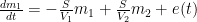
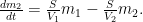
Those equations tell us that the carbon quantity 
![m_1(t) = \left[ \frac{V_1}{V_1+V_2}+\frac{V_2}{V_1+V_2} \exp\left(-\frac{V_1+V_2}{V_1V_2}St \right)\right] m_0 ,](https://s0.wp.com/latex.php?latex=m_1%28t%29+%3D+%5Cleft%5B+%5Cfrac%7BV_1%7D%7BV_1%2BV_2%7D%2B%5Cfrac%7BV_2%7D%7BV_1%2BV_2%7D+%5Cexp%5Cleft%28-%5Cfrac%7BV_1%2BV_2%7D%7BV_1V_2%7DSt+%5Cright%29%5Cright%5D+m_0+%2C+&bg=ffffff&fg=000&s=0&c=20201002)
which the substitutions 

Note that in the Fig. 2 system any constituent of the gas would be exchanged between vessels in accordance with the partial-pressure difference of that constituent alone, as if it were the only component the vessels contained. By thus constraining the flow from (and to) the first, atmosphere-representing vessel, this model supports the conclusion that the overall-carbon-dioxide quantity would, contrary to my previous argument, decay just as the excess, bomb-caused quantity of atmospheric carbon-14 did.

Could providing more than one sink enable us to escape that conclusion? Not necessarily. Consider the more-complex system that Fig. 3 depicts. Just as the system that my previous post described, this one can embody the TAR Bern-model parameters. As that post indicated, describing such a system requires a fourth-order linear differential equation. So that system does have more degrees of freedom in its initial conditions and can therefore exhibit a wider range of responses.
But it still constrains the flow among its four vessels linearly in accordance with partial pressures, just as the Fig. 2 system does. From complete equilibrium, therefore, its behavior for any constituent is the same as for any other constituent as well as for the contents as a whole. In other words, this model, too, seems to support the notion that the bomb-test results do indeed tell us how long excess carbon dioxide will remain if we stop taking advantage of fossil fuels.
In a sense, though, the models of Figs. 2 and 3 beg the question; they use the same uptake- and emissions-process-representing
So one question is how significant that difference is in the present context. I don’t have the answer, although my guess is, not very. But readers attempting to answer that question could do worse than start by referring to a previous WUWT post by Ferdinand Engelbeen.

Another way in which carbon-14 differs from the other two carbon isotopes is that it’s unstable. So, if the Fig. 3 model is adequate for carbon-12 or -13, a different model, which Fig. 4 depicts, would have to be used for carbon-14 if its radioactive decay is significant. That diagram differs from Fig. 3 in that it includes a flow 
To the extent that those different models produce different responses, using bomb-test data to predict the total carbon content’s behavior is problematic. But the Engelbeen post mentioned above seems to say that even deep-ocean residence times tend to be only a minor fraction of carbon-14’s half-life: this factor’s impact may be small.
A possibly more-significant factor is that the carbon cycle is undoubtedly non-linear, whereas the conclusions we tentatively drew from the models above depend greatly on their linearity. Before I reach that issue, though, I should point out an aspect of the Bern model that was not relevant to my previous post. The Bern equations I set forth in my last post were indeed linear. But that does not mean that their authors meant to say that the carbon cycle itself is. Although for the sake of simplicity I’ve discussed the models’ physical quantities as though they represented, e.g., the entire mass of carbon in a reservoir, their authors no doubt intended their (linear) models’ quantities to represent only the differences from some base, pre-industrial values. Presumably the purpose was to limit their range enough that the corresponding real-world behavior would approximate linearity.
But such linearization compromises the conclusions to which the models of Figs. 2 and 3 led us. A linear system is distinguished by the fact that its response to a composite stimulus always equals the sum of its individual responses to the stimulus’s various constituents; if the stimulus equals the sum of a step and a sine wave, for example, the system’s response to that stimulus will equal the sum of what its respective responses would have been to separate applications of the step and the sine wave. And this “superposition” property was central to drawing the conclusions we did from those models: the response to a large stimulus is proportionately the same as the response to a small one.

To appreciate this, consider Fig. 5, which depicts scaled values of the Fig. 2 model’s left-vessel total-carbon and carbon-14 contents. Initially, the system is at equilibrium, with zero outside emissions 


At time t = 5, a bolus of carbon-14 appears in the (atmosphere-representing) left vessel. Compared with the total carbon content, the added quantity is tiny, but it is large enough to double the small existing carbon-14 content. As the distance between the red dotted vertical lines shows, the resultant increase in carbon-14 content decays toward its new equilibrium value with a time constant of just about seven years. (I’ve assumed that the processes greatly favor the sink-representing right vessel—i.e., that its “volume” is much greater than the left vessel’s—so that the new equilibrium value is not much greater than the original.)
Now consider what happens at t = 45, when the left vessel’s total-carbon quantity suddenly increases. Although the two quantities are scaled to their respective initial values, this total-carbon increase is orders of magnitude greater than the t = 5 carbon-14 increase. Yet, as the black dotted vertical lines show, the decay of the left vessel’s total-carbon content proceeds just as fast proportionately as the much-smaller carbon-14 content did. As was observed above, this could tempt one to conclude that the carbon-14 decay we’ve observed in the real world tells us how fast the atmosphere would respond to our discontinuing fossil-fuel use.
![clip_image009[1]](http://wattsupwiththat.files.wordpress.com/2013/12/clip_image0091.png?quality=75 "clip_image009[1]")
But now consider what can happen if we relax the linearity assumption. Specifically, let’s say that the Fig. 2 model’s proportionality “constant”

In that plot, the red lines show that the carbon-14 decay occurs just as fast as in the previous plot, the carbon-14 content falling to exp(-1) above its new equilibrium value in around seven years. But the much-larger total-carbon increase brings the system into a lower-efficiency range, so that quantity subsides at a more-leisurely pace, taking over forty years. If such results are any indication, bomb-test results are a poor predictor of how long total-carbon content will settle.
Now permit me a digression in which I attempt to forestall pointless discussion of precisely what the quantities are that the graphs show. I believe the exposition is clearest if it is directed, as in Figs. 5 and 6, to ratios that carbon 14 and total carbon bear to their own initial values. But it appears customary to express the carbon-14 content instead in terms of its ratio to total carbon content. This means that, since total carbon has been increasing, the numbers commonly used in carbon-14 discussions could fall below the pre-bomb values, even though total carbon-14 has in fact increased.
For the sake of those to whom that issue looms large, I have attached Fig. 7 to illustrate how the values for carbon-14 itself could differ from those of its ratio to total carbon in a situation in which new (carbon-14-depleted) carbon is continually injected into the atmosphere.

But that’s a detail. More important is the issue that Fig. 6 raises.
Now, I “cooked” Fig. 6’s numbers to emphasize the point that nonlinearity can undermine conclusions based on linear models. Specifically, Fig. 6 depicts the results of making the flows proportional only to the fifth root of the carbon content.
But non-linearity must have some effect. How much? I don’t know. Together with the differences in behavior between carbon-14 and its stable siblings, though, it is among the considerations to take into account in assessing how informative the bomb-test data are.
As I warned at the top of the post, this post draws no conclusions from these considerations. But maybe the foregoing analysis will prompt knowledgeable readers’ comments that help narrow the issues.
hogwash….it’s the equivalent of the residence time of water in a sponge
It doesn’t matter how ‘high’ CO2 levels go…it’s not sustained
If it’s not replaced it still goes to zero
DocMartyn: “Now mechanistically we know that the atmosphere. V1, can ‘talk’ to the ocean surface, V3, but cannot ‘talk’ to the deep ocean, V4.”
Of course, deep-ocean water does have to come to the surface for interchange with the atmosphere. But looking at Mr. Engelbeen’s diagrams made me wonder whether the thermohaline circulation might result in behavior that mathematically is better matched by a model like the one you commented on in my last post.
I have no idea. But my (very brief) attempt to get the model above to match the Bern TAR behavior resulted in V values that didn’t immediately appeal to my intuition.
Michael, that is just plain nuts, but you don’t know that.
It’s too bad people like yourself NEVER got out more and experienced the REAL world, like a stint in the air force or the flying in the Navy, THEN you would not look so gullible and stupid posting material like this and making ridiculous claims, and this is sad, because, you *could* have something to contribute if and only if you were rational.
Sadly, you are not, rather, you appear to be ‘permanently wired’ for con spiracies not being able to work out the logistics (the material, the machines, and the men to carry it out) for the assertions (the ‘act’ of large scale or even small scale geo engineering) WHICH would show they are both highly improbable AND impractical.
Again, in your isolation, not associating with REAL people in the world (via church or social organizations or professional organizations; simply reading ZH does not count!)
Get a job, volunteer to work with the Red Cross or join some other civic organization and get some EXPOSURE to the rel world before its too late! Recovery will NOT become easier as you age … you don’t want to be known as a ‘raving nutter’ in your 60’s!!!!
.
DocMartyn says:
December 12, 2013 at 6:42 am
The connection between atmosphere and deep oceans is rather direct: sinks are going straight into the deep oceans and upwelling is also direct. Both are 5% of the total surface area of the oceans. For the rest of the oceans there is little connection between ocean surface and deep oceans, not in migration, not in temperature. There are exchanges by biolife, but as biolife in the oceans is not CO2 starved contrary to land plants, more CO2 in the oceans has no influence on biolife.
Therefore one can better see V3 and V4 as both directly connected to V1, which makes the calculations easier to follow with each their own exchange rates.
PS, CO2 movements between the oceans and the atmosphere are directly in ratio to the pCO2 difference between both: pCO2 is a measure for the number of CO2 molecules moving out of the water – for pCO2(aq) – or into the water – for pCO2(atm) -.
If pCO2(aq) = pCO2(atm) the same number of CO2 molecules get out as get in over the same time span…
[mods again… forgot the closing / tag in my previous message of December 12, 2013 at 7:06 am. Sorry again and thanks for your continuous effort]
I’m going to sit most of this one out, with popcorn, much as I love ODE systems linear or otherwise. I am far from convinced that the Bern model’s predictions of extremely long anthropogenic CO_2 residence times are correct, that the addition of previously sequestered carbon will substantially change the baseline equilibrium. But I’m also far from convinced that it won’t. Note well I’m also leaving out entirely a discussion of whether or not it will matter — the connection of climate catastrophe and increased CO_2 is highly speculative and not terribly well supported by ongoing empirical observation at the moment.
I will throw in one comment, however. All of the models above are linear, at least to leading order. As noted, linear models typically result in exponential decay, or in this case multiexponential decay, decay with many disparate time constants. That is, any “bolus” of CO_2 that enters the atmosphere should decay towards the current equilibrium. By (empirically) observing the time constant(s) of the decay of fluctuations, one (empirically) learns the dissipation rate(s) in the linear model. This is (in essence) the http://en.wikipedia.org/wiki/Fluctuation-dissipation_theorem, arguably the most underutilized non-equilibrium thermodynamic concept in climate science.
Sadly, the Mauna Loa data is nearly monotonic, with only the seasonal countervariation visible as a small wiggle on a weakly exponential (or, as noted, weakly quadratic as at this point the two are probably indistinguishable)growth. One could possibly infer seasonal uptake/outflow rates from the wiggles, although they are the average over two hemispheres of countervarying processes, but this will probably not give one the information one seeks about the overall rates, especially the rate at which CO_2 taken up and released at the ocean surface is equilibrated with the deep ocean and effectively sequestered in 4 C water (or, as noted, the rate at which previously sequestered CO_2 in the deep ocean is released where the cold waters upwell and are warmed). C14 is being used as a marker for a “bolus” not of absolute CO_2 but of CO_2 in a form that we can track directly as it is removed from the system. Sadly, this isn’t really a valid idea because (again to first order) the CO_2 removal mechanisms are likely to be insensitive to isotope, so all one obtains information on is a diffusion rate, not a removal rate. If I go and magically transmute a bunch of the CO_2 in one corner of my den into tagged C14-O_2 and then measure the C14-O_2 content of just the air in that corner, I’ll most definitely see it go down as the C14-O_2 diffuses into the rest of the air in the room, but that measurement will tell me next to nothing about how the CO_2 concentration in the room itself is varying. It will go down if the room CO_2 is constant. It will go down if the room CO_2 is increasing (as long as the increase isn’t more C14-O_2). It will go down if the room CO_2 is decreasing. This is because molecules from the rest of the room are diffusing in both directions — it is pure second law stuff.
The “room” in the current discussion is the entire system exclusive of “external” sources and sinks. External sources in this case are CO_2 created by burning stuff and chemical processes, CO_2 released from volcanoes and the Earth’s mantle (curiously excluded in the discussion above, curiously because various recent posts suggest that this source may not be in any sense negligible compared to anthropogenic contributions and we may not have the right order of MAGNITUDE of its contribution), and CO_2 from deep ocean upwelling (long time constant processes or immediate processes, the equivalent of me making beer in my den so that a fermenter filled with a previously stable organic compound — barley dextrose — is constantly adding new CO_2 to it at some rate). External sinks are pretty much the deep ocean — note that it is source and sink, but it is a HUGE source and HUGE sink with a VERY LONG time residence time and with multiple processes that can cause it to take up or release CO_2 — chemical processes within the ocean (creation of new carbonate shells, limestone) and the perpetual rain of dead ocean life from the upper surface that carries some of their carbon down to the deep sea bottom to eventually be subducted, to be tied up as methane and clathrates, to effectively be sequestered not really forever but for oceanic turnover timescales. The land biosphere COULD be a long time constant sink, but it is far more likely an anthropogenic source as we convert is previously long time constant stable turnover in the form of old-growth forests into short growth crops and timber sources.
At the moment I rather despair of being able to empirically determine the validity of the Bern model or any of the various alternatives capable of explaining the observational data equally well (it’s easy to explain a boring monotonic rise with a linear model. One might hope to learn something from events like the Gulf War (when many oil fields were torched, adding a bolus of CO_2 to the atmosphere) or when Gulf oil spill (where a supposedly huge amount of both oil and methane were released and where the methane at least should have ended up being a bolus of CO_2). Sadly, there isn’t a trace of them in the Mauna Loa data — no opportunity to use fluctuation-dissipation to learn something useful (at least, no opportunity that I would trust if you can’t eyeball an effect, even if a very sensitive program can find some associated statistical anomaly around those times). We cannot tell if the Mauna Loa increase is primarily from oceans still warming from the LIA with a century-scale time lag, from human CO_2, or from decadal-scale changes in deep ocean vulcanism. Even when surface boluses are released, by the time ML reads them they are well mixed and all we learn is that the CO_2 level in my den is slowly going up, not why or how long it is likely to remain resident.
So I share the frustration of Mr. Born. I have yet to be convinced by any argument that we really understand the baseline carbon cycle. It is fairly reasonable that human introduced CO_2 is contributing to the general increase, but it isn’t a slam-dunk by any means and offhand I don’t know how one could observationally confirm or falsify any of the really long term source or sink rates, especially if we haven’t even gotten vulcanism right to within orders of magnitude. If the Earth has been chasing near equilibrium (on the many and various timescales) with volcanoes that are a substantial source over geological time, then it is possible that we are substantially underestimating deep oceanic capacity and uptake rates and human contributions may be proportionally less important and/or have a much smaller resident lifetime than anticipated. Or not.
rgb
Ferdinand, you keep denying the data and concentrating on the mechanisms you know about.
The rule is analysis first, mechanism later.
This comment is stupid
“The connection between atmosphere and deep oceans is rather direct: sinks are going straight into the deep oceans and upwelling is also direct. Both are 5% of the total surface area of the oceans.”
If deep water makes its way to the surface it is surface water, if surface water makes its way to the depths, it become deep water. This potential flux is of course part of the V3 to V4 rate.
Joe, while non-linearity is well worth mentioning , I think it is something of a red-herring until we have a grasp on the more trivial, linear arguments.
I think figure is probably adequate and possibly vessel 2 may turn out to be expendible, within a good degree of approximation.
C14 decay is a minor issue that can be accounted for reasonably easily and accurately. Again probably a distraction until basic mechanism is roughed out.
Isotropic fractionation at atm/ocean surface likewise. It does matter (order of a few %) but not to first order guessing. Gosta states that C14 fractionation is about the same as C13 and this seems to be assumed in the C13 “correction” in the Nydal et al paper that goes with the airborne C14 data.
Probably the most important adjustment is Suess effect. ie dilution by emissions, that was already a notable effect before testing started but got drowned out by it. This could probably be ignored in the first 10 or so years after the test ban but then become more significant again.
Gosta is currently arguing (personal communication) that we should be looking at _number_ of C14 atoms, not C14 proportion (ppmv) and this changes the atm content curve.
This is a plot of the (C13 ‘corrected’) data as supplies by Nydal et al , ie ppm not number of C14. It may help concentrate minds to see it in detail.
http://climategrog.wordpress.com/?attachment_id=725
michaelwiseguy says:
December 11, 2013 at 10:29 pm
“OT but very funny and scary at the same time.
_________________________
So, David Keith says that his idea will kill 10,000 people a year in order to save the planet from Global Warming, but we will agree not to talk about it in polite society.
Got it.
stevefitzpatrick says:
December 12, 2013 at 5:46 am
Ferdinand,
You have the patience of a saint, but are you really making progress? There are none so blind as those who refuse to see.
Thanks a lot! Sometimes I think that I have better things to do (a lot of hobby’s – too many) than arguing the obvious, but as I see that this kind of totally outdated arguments come up again and again in debates with AGW proponents, that completely undermines the credibility of the skeptics who have much better defendable arguments where the AGW crowd is much weaker: the real impact of CO2 on climate, which is far below what most models “project”…
Thus I do my best to show my arguments to people who (still) want to listen, be it that some never will listen to any argument. That is the case for the extremes at either side of the fence…
Doc Martyn: “If deep water makes its way to the surface it is surface water, if surface water makes its way to the depths, it become deep water. This potential flux is of course part of the V3 to V4 rate.”
Be careful, this movement short circuits the model of series linked reservoirs. It may make more sense for vessel 2 to be a direct link to deep water. This is probably the cause of the 800y lag in the ice record. That is it has a 1/e time const of circa 800y and thus takes about 4000y to equilibrate.
It will equilbrate very quickly once at the surface but the physical mass movement and the massive reservoir makes it slow to respond.
Scrips Institude ‘cruise’ data shows upwelling deep water in Indian ocean to be a significant source of CO2
http://climategrog.wordpress.com/?attachment_id=715
DocMartyn says:
December 12, 2013 at 8:02 am
If deep water makes its way to the surface it is surface water, if surface water makes its way to the depths, it become deep water. This potential flux is of course part of the V3 to V4 rate.
As the surface area for the deep ocean sinks/sources is only 5% of the total surface, 95% of the ocean surface is bypassed and a large part of the V3 rate is bypassed by a V4 rate practically directly connected with V1.
RGB: “Sadly, the Mauna Loa data is nearly monotonic, with only the seasonal countervariation visible as a small wiggle on a weakly exponential (
or, as noted, weakly quadratic as at this point the two are probably indistinguishable)growth. One could possibly infer seasonal uptake/outflow rates from the wiggles, although they are the average over two hemispheres of countervarying processes, but this will probably not give one the information one seeks about the overall rates, ”
It’s only monotonic if you look at the integral accumulation. If you look at d/dt(CO2) it gets a lot more informative. And since it’s d/dt(CO2) that is affected by SST that is probably where we should be looking anyway.
http://climategrog.wordpress.com/?attachment_id=259
http://climategrog.wordpress.com/?attachment_id=233
Mike Jowsey says:
December 12, 2013 at 2:54 am
Isn’t open science fascinating?
___________________
Bless WUWT.
” Ferdinand
As the surface area for the deep ocean sinks/sources is only 5% of the total surface, 95% of the ocean surface is bypassed and a large part of the V3 rate is bypassed by a V4 rate practically directly connected with V1″
We have a language that has defined terms. Top and bottom have actual meanings, as do the phrases ‘deep water’ and ‘surface water’. Why do you want to destroy the accepted convention of what words actually mean? The interface between the atmosphere and the oceans is at the surface; period. The atmosphere does not meet the ocean anywhere else. In kinetic terms it does not matter a fetid dingoes kidney if CO2 is transported between the surface and depths by diffusion, unicorn’s pulling wagons loaded with DIC or by water currents; these are all parts of the flux between the surface and depths.
STOP mixing models and mechanisms; a little knowledge is a dangerous thing.
Thanks Joe Born. Food for thought.
Merry Christmas!
What a long post about nothing.
Plus (why he did it?) two equations which are actually only one.
The author is rather strange.
Of course C14 lifetime after a bomb explosion tells you nothing about the lifetime of anthropogenic CO2.
The bomb C14 was simply dissolved in the ocean forever and disappeared very fast.
There is very little C14 in the ocean otherwise.
The normal CO2 is in a quasi-equilibrium with the ocean. When the CO2-level slowly rises in the atmosphere, it means there is already a lot of CO2 dissolved additionally in the ocean. This dissolved CO2 will maintain the atmospheric CO2 level for hundreds or may be for thousands of years.
This is trivial.
In addition, the CO2 concerntration is described by a high order ODE, not by the baby-like first order one, as the author postulates.
Ferdinand Engelbeen: “Jquip, what goes into the deep oceans is the isotopic composition of today (minus some fractionation), what comes out of the deep oceans is the isotopic composition of ~1000 years ago (minus some fractionation and some radioactive dexay). That is irrelevant for what happens with a 12CO2 mass spike, but that is highly relevant for the 14CO2 concentration spike.”
At first this seems to make sense, but I haven’t been able to make the math work. Here’s my problem.
For eons, carbon-14 remains at a mass of 1000 in the atmosphere. It loses 100 every year to the Arctic Ocean (say) but receives 90 back every year from the Southern Ocean and has 10 added every year thanks to cosmic rays, so there’s no net change. (In this hypothetical the biosphere and mixed-ocean layers don’t exist. Also, magically, the Arctic Ocean emits no carbon dioxide, and the Southern Ocean absorbs none.) Now another 1000 is suddenly added, doubling the atmospheric content to 2000, but the Arctic Ocean responds by taking 200, while the Southern Ocean still is returning only 90 and the cosmic rays are still generating only 10. So the carbon-14 content decays by 100.
Now we’ll tell the same story, but this time we’re talking total carbon, of which the content has been 1000M for eons. It loses 100M every year to the Arctic Ocean but receives 100M back every year from the Southern Ocean, so its content remains the same. Now another 1000M is suddenly added, doubling the atmospheric content to 2000M, but the Arctic Ocean responds by taking 200M, while the Southern Ocean still is returning only 100M, so the total-carbon content decays by 100M.
The two quantities behaviors seem to parallel one another’s. What have I gotten wrong?
There ar eat least two missing “drain effects” on oceanic CO2 that are not accounted for. There is a drain rate due to the formation of limestone, and the drain rate due to algal formation of one type the most common type of Carbon by life, in the form of algal photosynthesis. Which in turn becomes plant and animal mass,and on death da significant proportion descends ot the abyssal depths.
So the fundamental equation is wrong due to the missing terms. In addition atmospheric CO2 is NOT anywhere near constant. Approximately in a proportion of 97 to 3 the CO2 is removed annually by some means of which presumably in a 30/70 the proportion is by land based CO2 sequestration, as well.
The results are significantly changed, far from reality.
The relevant issue is water.
98% of the CO2 in the lithosphere is dissolved in water as COC03.
The part pressure of gazeous CO2 in the athmosphe is a function of the proportion of CO2 in the water and its temperature (Henry’s law). Think cold beer, warm beer.
However much CO2 is injected into the athmosphere it will be dissolved in cold raindrops and cold surface water.
See the correlation between athmospheric background CO2 and SST since 1850 on http://www.biomind.de/realCO2/ , webiste of the late Ernst-Georg Beck.
Bless him for taking the trouble to collect, analyse and compile the data from direct measurements of athmospheric CO2 since the early 19th century!
Jquip: The utter allergy to approaching the simple math for either of these is wholly incomprehensible.
Simple compartment models with serious consideration of the rates (e.g. is CO2 uptake capacity-limited, zero-order or first-order?) are the minimum amount of consideration necessary to tackle this problem. Figures 6 and 7 by Joe Born illustrate why you can not simply think about this in terms of half-lives, and Ferdinand Engelbeen’s comments show what is necessary to start addressing the questions with any accuracy.
Thank you to Joe Born and Ferdinand Engelbeen for interesting posts.
rgb at duke, thank you for the link to the fluctuation-dissipation theorem.
Greg: “Gosta is currently arguing (personal communication) that we should be looking at _number_ of C14 atoms, not C14 proportion (ppmv) and this changes the atm content curve.”
I don’t understand that comment. As far as the atmosphere is concerned, I would have thought that, since carbon dioxide is such a small constituent of the atmosphere, the number of atoms would be almost exactly proportional to the number of parts per million.
Or were you talking about the distinction between Fig. 7’s red and green lines?
David Cole claims he has the answer to where the %50 split comes from. See his four part paper below:
http://bishophill.squarespace.com/storage/Atmospheric%20Carbon%20Dioxide%20Control%20Mechanisms-Part%201.pdf
http://www.bishop-hill.net/storage/Atmospheric%20Carbon%20Dioxide%20Control%20Mechanisms-Part%202.pdf
http://www.bishop-hill.net/storage/Atmospheric%20Carbon%20Dioxide%20Control%20Mechanisms-Part%203.pdf
http://www.bishop-hill.net/storage/Atmospheric%20Carbon%20Dioxide%20Control%20Mechanisms-Part%204%20_2_.pdf