
Guest post submitted by Ken Gregory, Friends of Science.org
An analysis of NASA satellite data shows that water vapor, the most important greenhouse gas, has declined in the upper atmosphere causing a cooling effect that is 16 times greater than the warming effect from man-made greenhouse gas emissions during the period 1990 to 2001.
The world has spent over $ 1 trillion on climate change mitigation based on climate models that don’t work. They are notoriously poor at simulating the 20th century warming because they do not include natural causes of climate change – mainly due to the changing sun – and they grossly exaggerate the feedback effects of greenhouse gas emissions.
Most scientists agree that doubling the amount of carbon dioxide (CO2) in the atmosphere, which takes about 150 years, would theoretically warm the earth by one degree Celsius if there were no change in evaporation, the amount or distribution of water vapor and clouds. Climate models amplify the initial CO2 effect by a factor of three by assuming positive feedbacks from water vapor and clouds, for which there is little direct evidence. Most of the amplification by the climate models is due to an increase in upper atmosphere water vapor.
The Satellite Data
The NASA water vapor project (NVAP) uses multiple satellite sensors to create a standard climate dataset to measure long-term variability of global water vapor.
NASA recently released the Heritage NVAP data which gives water vapor measurement from 1988 to 2001 on a 1 degree by 1 degree grid, in three vertical layers.1 The NVAP-M project, which is not yet available, extends the analysis to 2009 and gives five vertical layers.
From the NVAP project page:
The NASA MEaSUREs program began in 2008 and has the goal of creating stable, community accepted Earth System Data Records (ESDRs) for a variety of geophysical time series. A reanalysis and extension of the NASA Water Vapor Project (NVAP), called NVAP-M is being performed as part of this program. When processing is complete, NVAP-M will span 1987-2010. Read about changes in the new version.
Water vapor content of an atmospheric layer is represented by the height in millimeters (mm) that would result from precipitating all the water vapor in a vertical column to liquid water. The near-surface layer is from the surface to where the atmospheric pressure is 700 millibar (mb), or about 3 km altitude. The middle layer is from 700 mb to 500 mb air pressure, or from 3 km to 6 km attitude. The upper layer is from 500 mb to 300 mb air pressure, or from 6 km to 10 km altitude.
The global annual average precipitable water vapor by atmospheric layer and by hemisphere from 1988 to 2001 is shown in Figure 1.
The graph is presented on a logarithmic scale so the vertical change of the curves approximately represents the forcing effect of the change. For a steady earth temperature, the amount of incoming solar energy absorbed by the climate system must be balanced by an equal amount of outgoing longwave radiation (OLR) at the top of the atmosphere. An increase of water vapor in the upper atmosphere would temporarily reduce the OLR, creating a forcing of more incoming than outgoing energy, which raises the temperature of the atmosphere until the balance is restored.

Figure 1. Precipitable water vapor by layer, global and by hemisphere.
The graph shows a significant percentage decline in upper and middle layer water vapor from 1995 to 2001. The near-surface layer shows a smaller percentage increase, but a larger absolute increase in water vapor than the other layers. The upper and middle layer water vapor decreases are greater in the Southern Hemisphere than in the Northern Hemisphere.
Table 1 below shows the precipitable water vapor for the three layers of the Heritage NVAP and the CO2 content for the years 1990 and 2001, and the change.
| Layer | L1 near-surface | L2 middle | L3 upper | Sum | CO2 |
| 1013-700 | 700-500 | 500-300 | |||
| mm | mm | mm | mm | ppmv | |
| 1990 | 18.99 | 4.6 | 1.49 | 25.08 | 354.16 |
| 2001 | 20.72 | 4.03 | 0.94 | 25.69 | 371.07 |
| change | 1.73 | -0.57 | -0.55 | 0.61 | 16.91 |
Table 1. Heritage NVAP 1990 and 2001 water vapour and CO2.
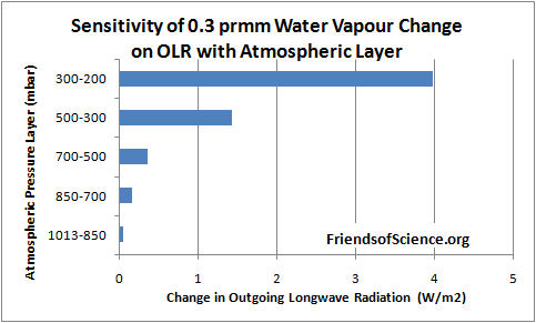
Dr. Ferenc Miskolczi performed computations using the HARTCODE line-by-line radiative code to determine the sensitivity of OLR to a 0.3 mm change in precipitable water vapor in each of 5 layers of the NVAP-M project. The program uses thousands of measured absorption lines and is capable of doing accurate radiative flux calculations. Figure 2 shows the effect on OLR of a change of 0.3 mm in each layer.
The results show that a water vapor change in the 500-300 mb layer has 29 times the effect on OLR than the same change in the 1013-850 mb near-surface layer. A water vapor change in the 300-200 mb layer has 81 times the effect on OLR than the same change in the 1013-850 mb near-surface layer.

Figure 2. Sensitivity of 0.3 mm precipitable water vapor change on outgoing longwave radiation by atmospheric layer.
Table 2 below shows the change in OLR per change in water vapor in each layer, and the change in OLR from 1990 to 2001 due to the change in precipitable water vapor (PWV).
| L1 | L2 | L3 | Sum | CO2 | ||
| OLR/PWV | W/m2/mm | -0.329 | -1.192 | -4.75 | ||
| OLR/CO2 | W/m2/ppmv | -0.0101 | ||||
| OLR change | W/m2 | -0.569 | 0.679 | 2.613 | 2.723 | -0.171 |
Table 2. Change of OLR by layer from water vapor and from CO2 from 1990 to 2001.
The calculations show that the cooling effect of the water vapor changes on OLR is 16 times greater than the warming effect of CO2 during this 11-year period. The cooling effect of the two upper layers is 5.8 times greater than the warming effect of the lowest layer.
These results highlight the fact that changes in the total water vapor column, from surface to the top of the atmosphere, is of little relevance to climate change because the sensitivity of OLR to water vapor changes in the upper atmosphere overwhelms changes in the lower atmosphere.
The precipitable water vapour by layer versus latitude by one degree bands for the year 1991 is shown in Figure 3. The North Pole is at the right side of the figure. The water vapor amount in the Arctic in the 500 to 300 mb layer goes to a minimum of 0.53 mm at 68.5 degrees North, then increases to 0.94 mm near the North Pole.

Figure 3. Precipitable water vapor by layer in 1991.
The NVAP-M project extends the analysis to 2009 and reprocesses the Heritage NVAP data. This layered data is not publicly available. The total precipitable water (TPW) data is shown in Figure 4, reproduced from the paper Vonder Haar et al (2012) here. There is no evidence of increasing water vapor to enhance the small warming effect from CO2.

Figure 4. Global month total precipitable water vapor NVAP-M.
The Radiosonde Data
Water vapor humidity data is measured by radiosonde (on weather balloons) and by satellites. The radiosonde humidity data is from the NOAA Earth System Research Laboratory here.

Figure 5. Global relative humidity, middle and upper atmosphere, from radiosonde data, NOAA Earth System Research Laboratory.
A graph of the global average annual relative humidity (RH) from 300 mb to 700 mb is shown in Figure 5. The specific humidity in g/kg of moist air at 400 mb (8 km) is shown in Figure 6. It shows that specific humidity has declined by 14% since 1948 using the best fit line.

Figure 6. Specific humidity at 400 mb pressure level
In contrast, climate models all show RH staying constant, implying that specific humidity is forecast to increase with warming. So climate models show positive feedback and rising specific humidity with warming in the upper troposphere, but the data shows falling specific humidity and negative feedback.
Many climate scientists dismiss the radiosonde data because of changing instrumentation and the declining humidity conflicts with the climate model simulations. However, the radiosonde instruments were calibrated and the data corrected for changes in response times. The data before 1960 should be regarded as unreliable due to poor global coverage and inferior instruments. The near surface radiosonde measurements from 1960 to date show no change in relative humidity which is consistent with theory. Both the satellite and radiosonde data shows declining upper atmosphere humidity, so there is no reason to dismiss the radiosonde data. The radiosonde data only measures humidity over land stations, so it is interesting to compare to the satellite measurements which have global coverage.
Comparison Between Radiosonde and Satellite Data
The specific humidity radiosonde data was converted to precipitable water vapor for comparison with the satellite data. Figure 7 compares the satellite data to the radiosonde data for the years 1988 to 2001.

Figure 7. Comparison between NOAA radiosonde and NVAP satellite derived precipitable water vapor.
The NOAA and NVAP data compares very well for the period 1988 to 1995. The NVAP satellite data shows less water vapor in the upper and middle layers than the NOAA data. In 2000 and 2001 the NVAP data shows more water vapor in the near-surface layer than the NOAA data. The vertical change on the logarithmic graph is roughly equal to the forcing effect of each layer, so the NVAP data shows water vapor has a greater cooling effect than the radiosonde data.
The Tropical Hot Spot
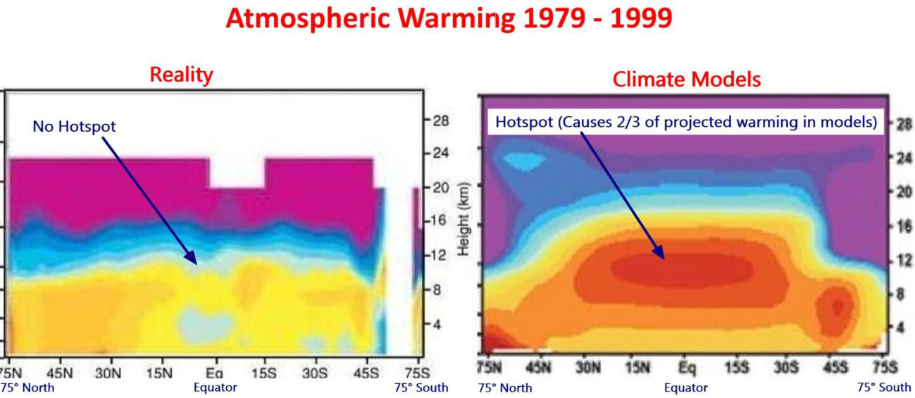
The models predict a distinctive pattern of warming – a “hot-spot” of enhanced warming in the upper atmosphere at 8 km to 13 km over the tropics, shown as the large red spot in Figure 8. The temperature at this “hot-spot” is projected to increase at a rate of two to three times faster than at the surface. However, the Hadley Centre’s real-world plot of radiosonde temperature observations from weather balloons shown below does not show the projected hot-spot at all. The predicted hot-spot is entirely absent from the observational record. If it was there it would have been easily detected.
The hot-spot is forecast in climate models due to the theory that the water vapor profile in the tropics is dominated by the moist adiabatic lapse rate, which requires that water vapor increases in the upper atmosphere with warming. The moist adiabatic lapse rate describes how the temperature of a parcel of water-saturated air changes as it move up in the atmosphere by convection such as within a thunder cloud. A graph here shows two lapse rate profiles with a larger temperature difference in the upper atmosphere than at the surface. The projected water vapor increase creates the hot-spot and is responsible for half to two-thirds of the surface warming in the IPCC climate models.

Figure 8. Climate models predict a hot spot of enhanced warming rate in the tropics, 8 km to 13 km altitude. Radiosonde data shows the hot spot does not exist. Red indicates the fastest warming rate. Source: http://joannenova.com.au
The projected upper atmosphere water vapor trends and temperature amplification at the hot-spot are intricately linked in the IPCC climate theory. The declining upper atmosphere humidity is consistent with the lack of a tropical hot spot, and both observations prove that the IPCC climate theory is wrong.
A recent technical paper Po-Chedley and Fu (2012) here compares the temperature trends of the lower and upper troposphere in the tropics from satellite data to the climate model projections from the period 1981 to 2008.2 The upper troposphere is the part of the atmosphere where the pressure ranges from 500 mb to 100 mb, or from about 6 km to 15 km. The paper reports that the warming trend during 1981 to 2008 in the upper troposphere simulated by climate models is 1.19 times the simulated warming trend of the lower atmosphere in the tropics. (Note this comparison is to the lower atmosphere, not the surface, and includes 10 years of no warming to 2008.) Using the most current version (5.5) of the satellite temperature data from the University of Alabama in Huntsville (UAH), the warming trend of the upper troposphere is only 0.973 of the lower troposphere in the tropics for the same period. This is different from that reported in the paper because the authors used an obsolete version (5.4) of the data. The satellite data shows not only a lack of a hot-spot, it shows a cold-spot just where a hot-spot was predicted.
Conclusion
Climate models predict upper atmosphere moistening which triples the greenhouse effect from man-made carbon dioxide emissions. The new satellite data from the NASA water vapor project shows declining upper atmosphere water vapor during the period 1988 to 2001. It is the best available data for water vapor because it has global coverage. Calculations by a line-by-line radiative code show that upper atmosphere water vapor changes at 500 mb to 300 mb have 29 times greater effect on OLR and temperatures than the same change near the surface. The cooling effect of the water vapor changes on OLR is 16 times greater than the warming effect of CO2 during the 1990 to 2001 period. Radiosonde data shows that upper atmosphere water vapor declines with warming. The IPCC dismisses the radiosonde data as the decline is inconsistent with theory. During the 1990 to 2001 period, upper atmosphere water vapor from satellite data declines more than that from radiosonde data, so there is no reason to dismiss the radiosonde data. Changes in water vapor are linked to temperature trends in the upper atmosphere. Both satellite data and radiosonde data confirm the absence of any tropical upper atmosphere temperature amplification, contrary to IPCC theory. Four independent data sets demonstrate that the IPCC theory is wrong. CO2 does not cause significant global warming.
Note 1. The NVAP data in Excel format is here.
Note 2. The lower troposphere data is: http://www.nsstc.uah.edu/public/msu/t2lt/uahncdc.lt
The upper troposphere data is calculated as 1.1 x middle troposphere – 0.1 x lower stratosphere; where middle troposphere is: http://www.nsstc.uah.edu/public/msu/t2/uahncdc.mt and the lower stratosphere is:http://www.nsstc.uah.edu/public/msu/t4/uahncdc.ls
============================================================
The original article is located at http://www.friendsofscience.org/index.php?id=483
Theo Goodwin says:
March 6, 2013 at 12:22 pm
You don’t need to know the value of feedbacks to calculate the no-feeback climate sensitivity. The no-feedback climate sensitivity to double CO2 is calculated by climate models where water vapor, clouds, ice, evaporation etc. are held constant. It is about 1 C.
The bottom line for separating science from nonsense is the recognition of massive model error or insignificant terms comprising the model. It is political science when the model errors don’t matter and the message continues on unabated.
Lance Wallace says:
March 6, 2013 at 12:39 pm
I provided a link to the Vonder Haar et al (2012) paper just above Figure 4.
What has been happening since 2001 ?
I would expect to see a cessation of the decline or a slight recovery
Some have argued for atmospheric heat energy to be used as a better and more meaningful metric than a supposed global mean temperature. Heat is a product of temp and water content. Viewed this way, decreasing water vapour could mean that increasing temperatures have not reflected increasing heat.
Rattus Norvegicus says:
March 6, 2013 at 1:28 pm
You are joking, right?!
The NVAP-M people released just the irrelevant total water vapor column even-year annual numbers only, but not the by-layered data. We don’t want to confuse the IPCC lead authors preparing the AR5 with inconvenient data!/sarc
Janice L. Bytheway, co-author of the Vonder Haar (2012) paper and NVAP-M team member wrote in an email to me 7/24/2012:
“As for your interest in the trends at the upper versus lower levels of the atmosphere, we unfortunately don’t have the staff or funding to provide subsets of the data at this time.”
A strange response since the total column amount is just the sum of the layers.
Again, this is the best available data. We expect that the data might improve, or be adjusted in the future, for better or worst. Of course we should use it, even if the result is embarrassing to the NASA team. They will get abuse from their climate alarmist colleagues, but we can hope it will not be as severe as what Phil Jones feared from his pals when he admitted there was a pause in global warming. Phil said “They will kill me!”
As the temperature standstill continues and evidence continues to trickle in that CAGW theory is failed, there is a sense of panic at the global warming centres of excellence dotted around the world. Pachauri will soon head off to greener pastures as he ralises the jig is up. Gore left the field some time last year (sold TV to oil, dumped green investments). As the scam unravels you will witness increased infighting as the rats bolt for the exits which are flooding with water.
Spanner in the works…but will not be discussed in the msm
At least one part of this story is completely wrong. The “friends of Science” link to the paper of Vonder Haar et al. (2012), the text of which is unfortunately behind a pay-wall. The article states:
The strength of the NVAP-M dataset is its global overview of humidity. Because the number and types of the satellites change during the period studied and because the orbit of the satellites change during their life time, the dataset is not homogenenous. They did work on improving the homogeneity of the data, but this work is not finished. Its trends should not be interpreted.
This should have been known with Anthony Watts. Forest Mims above links to his guest post about the NVAP-M dataset. Already here I have explained in the comments that the authors of the NVAP-M dataset do not think their data can be used for trend analysis.
“Trying not to be a conspiracy nut, but since NASA is a government funded organization, and US taxpayers fund it i.e. – We paid for this information. Why and who has been sitting on this information for the entire “Global Warming” time period. The data start in 1988 and from the shown graph by 1995 the “causes more water” theory was shot down.
Talk about hide the decline.”
Hear, hear! NASA is sitting on this as it will end Hansen, expose a lot of nonsense in a lot of models, and rearrange a lot of people’s careers. Wonder if Obomination has anything to do with it? He does have his fingers in a lot of pies. FOIA, anyone? Ken Gregory, you know where the bodies are buried?
That’s weird my other post got lost.
“Maybe the water vapour is not making it to the upper layer.”, i postulated; then i cited a few youtube posts about “record snowfall 2013”, and “russia snowfall 2013″…one example from North America, Russia, and Japan. But i accidentally used the wrong URL for the Japan example, instead i referenced to a record breaking snowball fight in Utah (this was a cool clip).
Ken Gregory says:
March 6, 2013 at 2:39 pm
“….You don’t need to know the value of feedbacks to calculate the no-feeback climate sensitivity. The no-feedback climate sensitivity to double CO2 is calculated by climate models where water vapor, clouds, ice, evaporation etc. are held constant. It is about 1 C.”
/////////////////////////////////////////////////////////////////////////////////
But we live in the real world, and what is relevant to the real world is the effect of feedbacks on that ‘theoretical’ figure. If these feedbacks are negative then less than 1C will enure, and if positive then more that 1C will enure.
If one looks at the satellite data (33 years) if one removes the 1998 super El Nino (which no-one suggests was caused by CO2) then first order correlation with CO2 emissions over those 33 years is essentially zero (flat between 1979 and 1997 and flat between 1998 to 2012). This data therefore supports the view that feedbacks may well be negative.
Moderators CORRECTION, plse
Ken Gregory says:
March 6, 2013 at 2:39 pm
“….You don’t need to know the value of feedbacks to calculate the no-feeback climate sensitivity. The no-feedback climate sensitivity to double CO2 is calculated by climate models where water vapor, clouds, ice, evaporation etc. are held constant. It is about 1 C.”
/////////////////////////////////////////////////////////////////////////////////
But we live in the real world, and what is relevant to the real world is the effect of feedbacks on that ‘theoretical’ figure. If these feedbacks are negative then less than 1C will enure, and if positive then more that 1C will enure.
If one looks at the satellite data (33 years) if one removes the 1998 super El Nino (which no-one suggests was caused by CO2) then first order correlation with CO2 emissions over those 33 years is essentially zero (flat between 1979 and 1997 and flat between 1999 to 2012). This data therefore supports the view that feedbacks may well be negative.
phlogiston says:
March 6, 2013 at 3:09 pm
Ya, it could be called Earth Enthalpy (EE). Then the anomaly in enthalpy could be referred to as exo or endo…i love it!!! EEE or EEE*
That would be a great metric for Global Whatever!
Berényi Péter says:
March 6, 2013 at 1:53 pm
The reason water vapor distribution is a fractal is that water vapor content of each parcel is determined by its history, that is, by its temperature the last time it got saturated. This event might have occurred several days or weeks ago. In the meantime turbulent flows distorted that, originally bulky parcel into a mesh of thin threads, interwoven by other parcels of a completely different history. That’s how water vapor distribution looks like at any specific moment and this is why shape of clouds is always fractal-like, for the “surface” of a cloud is nothing else but the surface separating a region of saturation from others with lower relative humidity. Geometry of each constant relative humidity surface is like that, even if most of them are invisible to the naked eye.
Bold emphasis is mine. This is an interesting concept… one I had not considered before. Thank you for this insight BP!
MtK
DD More says:
March 6, 2013 at 1:55 pm
>>>>>>>>>>>>>>>>>>>>>>>>>>>
Keep trying!
Scientific information has become proprietary.
Enough Americans have been objecting to this lately the gov agreed to allow limited access (12 months) on some scientific research, but they haven’t followed through on this (that im aware). We will see (hopefully) if there is granted access or that a surprising amount of science is really classified…at least then we would know hahaha
Viz: Laurie Bowen post:
http://wattsupwiththat.com/2013/02/22/king-obama-to-circumvent-lawful-due-process-on-climate/#comment-1231260
In Canada, the scientists are leaking to the press that they have been muzzled as a condition of employment. Whistleblowers Preventative measures, excellent.
http://sciencewriters.ca/initiatives/muzzling_canadian_federal_scientists/
“An analysis of NASA satellite data shows that water vapor, the most important greenhouse gas, has declined in the upper atmosphere”
So I guess that next NASA will be telling us where that water has gone, and that the polar ice caps and glaciers are in fact growing…. Or are they going to tell us that this missing water is ALSO hiding at the bottom of the ocean….
It would be nice to see the 2001 data plotted on figure 3 with the 1991 data.
Thanks for the post.
Water vapor (and cloud) feedback is the make or break for this general theory.
These ARE the most important aspects to consider and measure regarding if there will be significant global warming from GHG increases or not. They really are.
So far, they appear to be around Zero (maybe slightly positive or maybe slightly negative).
If they do turn out to be Zero (or slightly positive or slightly negative), warming is nothing to worry about. This issue raised by Ken is the most important one there is regarding this theory.
One might have to do the math in terms of how the feedbacks multiply on top of each other to get us up to 3.0C per doubling and how small changes in these feedback on feedback values would leave completely different results but this point should not be under-estimated. If I was in the conspiracy camp, I might conclude the feedback impacts were carefully tuned to reach a 3.0C per doubling level rather than determined based on how the climate operates.
Don’t worry we’ll just have a nuclear winter to offset the global warming – will all balance out nicely …according to the models of course ….
[snip – I suggest you try again without the accusations Joel – Anthony]
Note the declining atmospheric water vapour over the last 20 years is also shown in Forrest M. Mims III’s work
http://www.forrestmims.org/sciencedata.html
Total Column Water Vapor (1990 to 2010)
Have you submitted this for publication?
Ken Gregory says:
March 6, 2013 at 1:26 pm
Justthinkin says:
March 6, 2013 at 11:50 am
Ken…thank you for the reply….I may be a bit old, but I was taught in aeronautical engneering,the lower the temp diff between the poles and the equator,the less severe the weather. The way my prof from the RCAF(which shows how old I am) put it…in layman’s terms….when a male and female are both hot to trot,less resistance,disturbance,and more friction (which is good),therefore less turbulance and storms. A bit crude,but to the point.And yes,I do know the diff between vapour and liquid..should have added the /sarc tag. Mea Culpa.
Meh. Probably will, except alarmists will claim that reduced water vapour is a sign of impending doom and desertification caused by a different more dangerous, worse than we thought type of co2.