Guest essay by Joe Born
In a recent post Christopher Monckton identified me as a proponent of the following proposition: The observed decay of bomb-generated atmospheric-carbon-14 concentration does not tell us how fast elevated atmospheric carbon-dioxide levels would subside if we discontinued the elevated emissions that are causing them. He was entirely justified in doing so; I had gone out of my way to bring that argument to his attention.
But I was merely passing along an argument to which a previous WUWT post had alerted me, and the truth is that I’m not at all sure what the answer is. Moreover, semantic issues diverted the ensuing discussion from what Lord Monckton probably intended to elicit. So, at least in my view, we failed to join issue.
In this post I will attempt to remedy that failure by explaining the weakness that afflicts the position attributed (again, understandably) to me. I hasten to add that I don’t profess to have the answer, so be forewarned that no conclusion lies at the end of this post. But I do hope to make clearer where at least this layman thinks the real questions lie.

To start off, let’s review the argument I made, which is that the atmospheric-carbon-dioxide turnover time is what determined how long the post-bomb-test excess-carbon-14 level took to decay. That argument was based on the “bathtub” model, which Fig. 1 depicts. The rate at which the quantity <i>m</i> of water the tub contains changes is equal to the difference between the respective rates <i>e</i> (emissions) and <i>u</i> (uptake) at which water enters from a faucet and leaves through a drain:

The same thing can, <i>mutatis mutandis</i>, be said of contaminants (read carbon-14) in the water. But in the case of well-mixed contaminants one of the <i>mutanda</i> is that the rate at which the contaminants leave is dictated by the rate at which water leaves:

where 

Consequently, if the water quantity increases for an interval during which <i>e</i> exceeds <i>u</i>, it will thereafter remain elevated if the emissions rate <i>e</i> then falls no lower than the drain rate <i>u</i>. If a dose of contaminants is added to the water, though, the resultant contaminant amount falls, even when there’s no difference between <i>u</i> and <i>e</i>, in accordance with the <i>turnover</i> rate, i.e., with the ratio of <i>u</i> to <i>m</i>. So, to the extent that this model reflects reality’s relevant aspects, we can conclude that the rate at which the carbon-14 concentration decays tells us nothing about what happens when total-CO2 emissions return to a “normal” level.
But among the foregoing model’s deficiencies is that it says nothing about a possible dependence of overall drain rate <i>u</i> on the water quantity <i>m</i>, whereas we may expect biosphere uptake (and emissions) to respond to the atmosphere’s carbon-dioxide content. Nor does it deal with the possibility that after contamination has flowed out the drain it will be recycled through the faucet. In contrast, the biosphere no doubt returns to the atmosphere at least some of the carbon-14 it has previously taken from it.

A model that takes such factors into account could support a conclusion different from the one to which the bathtub led us. Consistently with my last post’s approach, Fig. 2 uses interconnected pressure vessels to represent one such model. In this case there are only two vessels, the left one representing the atmosphere and the right one representing carbon sinks such as the ocean and the biosphere.
The vessels contain respective quantities 


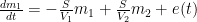
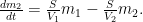
Those equations tell us that the carbon quantity 
![m_1(t) = \left[ \frac{V_1}{V_1+V_2}+\frac{V_2}{V_1+V_2} \exp\left(-\frac{V_1+V_2}{V_1V_2}St \right)\right] m_0 ,](https://s0.wp.com/latex.php?latex=m_1%28t%29+%3D+%5Cleft%5B+%5Cfrac%7BV_1%7D%7BV_1%2BV_2%7D%2B%5Cfrac%7BV_2%7D%7BV_1%2BV_2%7D+%5Cexp%5Cleft%28-%5Cfrac%7BV_1%2BV_2%7D%7BV_1V_2%7DSt+%5Cright%29%5Cright%5D+m_0+%2C+&bg=ffffff&fg=000&s=0&c=20201002)
which the substitutions 

Note that in the Fig. 2 system any constituent of the gas would be exchanged between vessels in accordance with the partial-pressure difference of that constituent alone, as if it were the only component the vessels contained. By thus constraining the flow from (and to) the first, atmosphere-representing vessel, this model supports the conclusion that the overall-carbon-dioxide quantity would, contrary to my previous argument, decay just as the excess, bomb-caused quantity of atmospheric carbon-14 did.

Could providing more than one sink enable us to escape that conclusion? Not necessarily. Consider the more-complex system that Fig. 3 depicts. Just as the system that my previous post described, this one can embody the TAR Bern-model parameters. As that post indicated, describing such a system requires a fourth-order linear differential equation. So that system does have more degrees of freedom in its initial conditions and can therefore exhibit a wider range of responses.
But it still constrains the flow among its four vessels linearly in accordance with partial pressures, just as the Fig. 2 system does. From complete equilibrium, therefore, its behavior for any constituent is the same as for any other constituent as well as for the contents as a whole. In other words, this model, too, seems to support the notion that the bomb-test results do indeed tell us how long excess carbon dioxide will remain if we stop taking advantage of fossil fuels.
In a sense, though, the models of Figs. 2 and 3 beg the question; they use the same uptake- and emissions-process-representing
So one question is how significant that difference is in the present context. I don’t have the answer, although my guess is, not very. But readers attempting to answer that question could do worse than start by referring to a previous WUWT post by Ferdinand Engelbeen.

Another way in which carbon-14 differs from the other two carbon isotopes is that it’s unstable. So, if the Fig. 3 model is adequate for carbon-12 or -13, a different model, which Fig. 4 depicts, would have to be used for carbon-14 if its radioactive decay is significant. That diagram differs from Fig. 3 in that it includes a flow 
To the extent that those different models produce different responses, using bomb-test data to predict the total carbon content’s behavior is problematic. But the Engelbeen post mentioned above seems to say that even deep-ocean residence times tend to be only a minor fraction of carbon-14’s half-life: this factor’s impact may be small.
A possibly more-significant factor is that the carbon cycle is undoubtedly non-linear, whereas the conclusions we tentatively drew from the models above depend greatly on their linearity. Before I reach that issue, though, I should point out an aspect of the Bern model that was not relevant to my previous post. The Bern equations I set forth in my last post were indeed linear. But that does not mean that their authors meant to say that the carbon cycle itself is. Although for the sake of simplicity I’ve discussed the models’ physical quantities as though they represented, e.g., the entire mass of carbon in a reservoir, their authors no doubt intended their (linear) models’ quantities to represent only the differences from some base, pre-industrial values. Presumably the purpose was to limit their range enough that the corresponding real-world behavior would approximate linearity.
But such linearization compromises the conclusions to which the models of Figs. 2 and 3 led us. A linear system is distinguished by the fact that its response to a composite stimulus always equals the sum of its individual responses to the stimulus’s various constituents; if the stimulus equals the sum of a step and a sine wave, for example, the system’s response to that stimulus will equal the sum of what its respective responses would have been to separate applications of the step and the sine wave. And this “superposition” property was central to drawing the conclusions we did from those models: the response to a large stimulus is proportionately the same as the response to a small one.

To appreciate this, consider Fig. 5, which depicts scaled values of the Fig. 2 model’s left-vessel total-carbon and carbon-14 contents. Initially, the system is at equilibrium, with zero outside emissions 


At time t = 5, a bolus of carbon-14 appears in the (atmosphere-representing) left vessel. Compared with the total carbon content, the added quantity is tiny, but it is large enough to double the small existing carbon-14 content. As the distance between the red dotted vertical lines shows, the resultant increase in carbon-14 content decays toward its new equilibrium value with a time constant of just about seven years. (I’ve assumed that the processes greatly favor the sink-representing right vessel—i.e., that its “volume” is much greater than the left vessel’s—so that the new equilibrium value is not much greater than the original.)
Now consider what happens at t = 45, when the left vessel’s total-carbon quantity suddenly increases. Although the two quantities are scaled to their respective initial values, this total-carbon increase is orders of magnitude greater than the t = 5 carbon-14 increase. Yet, as the black dotted vertical lines show, the decay of the left vessel’s total-carbon content proceeds just as fast proportionately as the much-smaller carbon-14 content did. As was observed above, this could tempt one to conclude that the carbon-14 decay we’ve observed in the real world tells us how fast the atmosphere would respond to our discontinuing fossil-fuel use.
![clip_image009[1]](http://wattsupwiththat.files.wordpress.com/2013/12/clip_image0091.png?quality=75 "clip_image009[1]")
But now consider what can happen if we relax the linearity assumption. Specifically, let’s say that the Fig. 2 model’s proportionality “constant”

In that plot, the red lines show that the carbon-14 decay occurs just as fast as in the previous plot, the carbon-14 content falling to exp(-1) above its new equilibrium value in around seven years. But the much-larger total-carbon increase brings the system into a lower-efficiency range, so that quantity subsides at a more-leisurely pace, taking over forty years. If such results are any indication, bomb-test results are a poor predictor of how long total-carbon content will settle.
Now permit me a digression in which I attempt to forestall pointless discussion of precisely what the quantities are that the graphs show. I believe the exposition is clearest if it is directed, as in Figs. 5 and 6, to ratios that carbon 14 and total carbon bear to their own initial values. But it appears customary to express the carbon-14 content instead in terms of its ratio to total carbon content. This means that, since total carbon has been increasing, the numbers commonly used in carbon-14 discussions could fall below the pre-bomb values, even though total carbon-14 has in fact increased.
For the sake of those to whom that issue looms large, I have attached Fig. 7 to illustrate how the values for carbon-14 itself could differ from those of its ratio to total carbon in a situation in which new (carbon-14-depleted) carbon is continually injected into the atmosphere.

But that’s a detail. More important is the issue that Fig. 6 raises.
Now, I “cooked” Fig. 6’s numbers to emphasize the point that nonlinearity can undermine conclusions based on linear models. Specifically, Fig. 6 depicts the results of making the flows proportional only to the fifth root of the carbon content.
But non-linearity must have some effect. How much? I don’t know. Together with the differences in behavior between carbon-14 and its stable siblings, though, it is among the considerations to take into account in assessing how informative the bomb-test data are.
As I warned at the top of the post, this post draws no conclusions from these considerations. But maybe the foregoing analysis will prompt knowledgeable readers’ comments that help narrow the issues.
Having studied archaeology, C14 is a radioactive isotope that is absorbed by all organic matter. Then it decays slowly. It has fluctuated over the years because of sun spot activity that deflect galactic sub atomic particles bombarding the earth. The same sub atomic particles also when they meld with water vapor molecules form clouds. I don’t know if it is correct, but before they banned atmospheric Atom and Hydrogen bombs the C.14 increased. We had terrible weather too lots of rain and cold temps in UK. That is why any carbon 14 dating usually gets a + or minus, and anything younger than say 2,000 is harder to date accurately and other dating methods have to be used.
OT but very funny and scary at the same time.
Stephen Colbert Tells David Keith Government is Already Spraying Us « GeoEngineering Exposed
Connecting CO2 sources/sinks in the manner shown here is analogous to the way an electrical engineer might connect multiple resistors and capacitors in a network without using any active elements (amplifiers or buffers). Because you can never achieve complex poles with this restriction, the resulting low-pass filters are not very useful (frequency characteristics are way too wimpy). We don’t do it that way.
This is NOT to suggest that the electrical equivalents could not be completely correct and very useful as models for CO2 migrations. The mathematics (that is – the physics) is very similar if not identical.
While NOT very useful for usual signal processing (analog filtering here) we do use these schemes for “envelope generators” for electronic music generation as I have recently reviewed at
http://electronotes.netfirms.com/EN210.pdf
[ In synthesizer design, “envelopes” are slowly-varying contours (way sub-audio) which are the parameters or controls for single tones (single notes).] My summary referenced here shows four approaches to solutions: the differential equation approach (eigen-analysis), but also the corresponding Laplace transform method, numerical simulation solutions, and finally a (gasp!) experiment. This comparison smorgasbord may be of interest here.
seeing as temperature over the history of the earth has changed dramatically, and the CO2 has changed with that temperature with a lag, then who cares. it seems rather obvious that the earth was & still is capable of absorbing CO2 in cooling conditions, so really it must be linear or something close to it or earth would not have survived as we know it.
Hopelessly over complicated. From Fig 5 and discussion, I question whether the writer understands the system we are talking about. 14C is effectively a tracer. There is a steady state level maintained by adding the same amount to the atmosphere each year from transmutation via cosmic ray interactions with nitrogen atoms in the atmosphere. The total amount of carbon is essentially unchanged. The atomic bombs did not increase the amount of CO2 in the atmosphere, but did almost double the tiny amount of 14C.
A basic reasonable assumption of a single turnover kinetics is the tracer leaves the reservoir and does not come back. 14C leaving the atmosphere can safely be assumed to not return in any significant fraction. Hence, when we see it leave, that is the off rate cleanly determined. Now when we have an equilibrium level, we can calculate the on rate as well. It doesn’t matter how complicated the reservoir system you create. The only part that matters is the off rate constant. We don’t know how the material partitions into other reservoirs, but that issue is beyond the scope of this experiment.
I showed previously [1] the math works out nicely, and essentially you can slice off the steady-state amount of 14C and look at the decay of the excess alone. The t1/2 is about 5 years. Even accounting for the increase in ppmv CO2 diluting the 14C from 1963 to 1993 and beyond, the t1/2 is still about 5 years (at least it was in my hands). Once you know the t1/2 is 5 years, a number of interesting calculations follow.
For one thing, it becomes pretty clear the increase in atmospheric CO2 cannot possibly be due to anthropogenic CO2. The CO2 quantity changes simply don’t match what humans have produced given the amount of CO2 we have produced each year from the late 1700s and how much would be left Y years after emission.
1) http://wattsupwiththat.com/2013/11/21/on-co2-residence-times-the-chicken-or-the-egg/#comment-1481426
Dear Joe,
By thus constraining the flow from (and to) the first, atmosphere-representing vessel, this model supports the conclusion that the overall-carbon-dioxide quantity would, contrary to my previous argument, decay just as the excess, bomb-caused quantity of atmospheric carbon-14 did.
The main problem with that model is that there is no lag included between the outflow (from the atmosphere in the deep oceans) and the inflow (from the deep oceans to the atmosphere). That makes that there is not only a huge difference in mass, but also a huge difference in concentrations of 14C.
What goes into the deep oceans is in direct ratio to the partial pressure difference of CO2 between atmosphere and ocean surface. What comes out is in direct ratio to the partial pressure difference of CO2 between ocean surface and atmosphere. That is the same for 12CO2 and 14CO2, with a small difference due to kinetics.
What goes into and comes from the deep oceans is thus directly related to their relative partial pressure differences.
For 12CO2 that is about 97% (in mass) * 99% (in concentration) that returns of what is going into the deep oceans, but for 14CO2, that is only 97% (in mass) * 45% (in concentration) at the time of the peak bomb test (1960):
http://www.ferdinand-engelbeen.be/klimaat/klim_img/14co2_distri_1960.jpg
The mass difference in this scheme is only at the inputs (to make the difference clear), but in reality it is equally distributed between deep ocean input and output to/from the atmosphere.
In pre-industrial times about 90% (45% of the bomb spike) of 14CO2 returned from the deep oceans for a ~1000 years lag, but that was about compensated by fresh production from cosmic rays.
Thus the 14CO2 decay is a mix of the mass spike decay (about equal to a 12CO2 mass spike decay) which depends of the atmospheric partial pressure and the “contamination” spike decay, which depends of the residence time.
That makes that the 14CO2 bomb spike decay rate of ~14 years is longer that the residence time, but shorter than the decay rate of a 12CO2 mass spike.
Something similar happens to the 13CO2 rate decay caused by the use of low-13C fossil fuels. If we look at the decrease of the 13C/12C ratio in the atmosphere, we see a decay rate which is only 1/3rd of what can be expected from the use of fossil fuels. That too is caused by the “thinning” from 13C-rich upwelling waters from the deep oceans. That can be used to estimate the deep ocean – atmosphere exchanges over a year:
http://www.ferdinand-engelbeen.be/klimaat/klim_img/deep_ocean_air_zero.jpg
or about 40 GtC/year in and out between atmosphere and deep oceans.
With that in mind, the residence times of a “human” CO2 spike can be estimated if we give a pulse of 13c-depleted CO2 of 100 GtC to the pre-industrial CO2 level of 580 Gtc:
http://www.ferdinand-engelbeen.be/klimaat/klim_img/fract_level_pulse.jpg
where FA is the fraction of “human” CO2 in the atmosphere, FL in surface waters, tCA total carbon in the atmosphere and nCA natural carbon in the atmosphere.
After ~60 years all low-13C from fossil fuels is replaced by “natural” CO2 from the deep oceans, while still 45% of the original total CO2 spike is present…
Hoser says:
December 11, 2013 at 11:32 pm
Your calcualtion is for the thinning of 14CO2 by the total CO2 turnover, which gives you the residence time (which is mainly temperature difference dependent), but that has nothing to do with the decay time for a mass pulse (which is mainly pressure difference dependent).
It is nothing humans can control anyway.
I’m grateful to Mr. Born for his detailed consideration of the CO2-lifetime question..The literature from Revelle onwards supports Hoser’s contention that the turnover time is 5-7 years: but that, as Mr. Engelbeen reminds us, is not the whole story. Dick Lindzen estimates that most CO2 molecules added to the atmosphere will have found their way out of it again in about 40 years. That is below the IPCC’s 50-200 years.
And the missing sink remains missing. Why is half of all the CO2 we emit disappearing instantaneously from the atmosphere? I’d be most grateful if wiser heads than mine were able to explain that.
Ferdinand Engelbeen says:
December 12, 2013 at 12:27 am
Hoser says:
December 11, 2013 at 11:32 pm
Your calcualtion is for the thinning of 14CO2 by the total CO2 turnover, which gives you the residence time (which is mainly temperature difference dependent), but that has nothing to do with the decay time for a mass pulse (which is mainly pressure difference dependent).
NO NO NO NO NO NO NO NOOOOOO! (adopts facial expression of The scream by Munch)
Ferdninand we all respect your erudition in regard to atmospheric CO2 but I fully agree here with Hoser that all this discussion is completely missing what a radio tracer measurement really is. And vastly over-complicating the discussion as a result.
A radiotracer measures a single removal term. PERIOD. A pulse of CO2 enters the atmosphere different from the other CO2 due to 14C. So it can be tracked in exclusion of any other CO2.
It is COMPLETELY IRRELEVANT all the other cycling and dilution and dynamics, pressure, temperature etc. of CO2 that are going on, the 14 tracer simply tells us the removal term for CO2. That is the whole point of a radiotracer measurement.
From the bomb test data we know that:
CO2 removal half life = 5 years
CO2 residence time = half life / ln2 = 5 / 0.693 = 7.7 years
That is the WHAT. Everything else is the WHY.
Cl4 can not be absorbed once the organism dies, or is buried. So that is how they can calculate by the amount of half life remaining how old the organism is. Anything organic including bones, trees etc., that have been unearthed in an archaeological site. I can’t see the problem really, we are bombarded all the time by galactic sub atomic particles. When sun pot activity is large then we don’t receive as much. Inactive and we receive a lot, including more clouds.
As a layman reading this it seems to over complicate the issue but you will see my ignorance shine through from my comment ! C14 as a tracer should provide a reasonable means of tracking the removal or sequestration rate of CO2.
We know from NASA that higher levels of CO2 have resulted in an increase of ~15% in vegetative matter globally which has ‘captured’ and removed CO2, although I don’t know if any calculations or studies show the likely amount of CO2 by weight and percentage that is. I assume there must be and that forward projections of increased rates of capture in higher CO2 levels are there somewhere. As an aside – I wonder if the increase in tree growth and number of leaves increases the release rate of volatile organics which in turn serve to increase forest related cloud formation and increased rainfall – or maybe with less water requirement (elevated CO2 and fewer stoma) they respond by producing less VO ?
Bacteria (some anyway) capture carbon and there is a strong likelihood that the populations of these may explode or implode depending on ambient CO2 levels which suit them best, again I don’t know if this has been studied or evaluated although it potentially may have very dramatic effects on the rate of carbon sequestration. Ditto bacteria which emit CO2.
I cannot see how the ‘bath tub’ simile has any value at all without including a means to show some form of active sequestration within the first bath tub. As you can see I am filled with curious ignorance.
Joe Born: “The observed decay of bomb-generated atmospheric-carbon-14 concentration does not tell us how fast elevated atmospheric carbon-dioxide levels would subside if we discontinued the elevated emissions that are causing them.”
Yes, but as Lubos Motl has pointed out, we can easily calculate this rate without bothering with 14C.
Lubos Motl says:
November 22, 2013 at 1:42 am
“It’s trivial to see that the residence time of CO2 is of order 30 years or longer. We emit 4 ppm worth of CO2 a year; the CO2 concentration increases by 2 ppm per year. So it’s clear that the “excess uptake” (which is natural and depends on the elevated CO2 relatively to the equilibrium) is also 2 ppm pear year. The excess CO2 above the equilibrium value for our temperature- which is still around 280 ppm – is about 120 ppm so one needs about 30 years to halve the excess CO2 and 50 years to divide it by e.”
Residence time τ can been defined (Barth, 1952, quoted by Henderson, 1982§) as τ = A/(dA/dt), where A is the amount of a substance dissolved or contained in a reservoir and dA/dt is the rate of efflux of that substance from the reservoir. In the case here considered the ‘substance’ can be considered as the excess atmospheric CO2 above the equilibrium value for today’s temperatures (around 280ppm). So if today’s CO2 concentration is about 400ppm, then A = 400 – 280 = 120ppm.
If (as Lubos states) the equivalent of 4ppm excess (i.e. anthropogenic) CO2 is being emitted to the atmosphere annually, while the concentration in the atmosphere is increasing by 2ppm/year, then dA/dt = 2ppm/year and τ (the residence time in the atmosphere of the excess CO2) is 120/2 years, so 60 years. Of course that assumes that anthropogenic omissions cease now, which they won’t…but any talk of residence time being less than 10 years is unrealistic.
§ Henderson, P. 1982. Inorganic geochemistry. p. 287.
Ferdinand Engelbeen:
Thank you very much for the response. I’m going to have to get some coffee in me before I digest it all, but it seems to me that your third graph is actually your answer to the ultimate question. I think I’ll have questions about how you get there, but I won’t impose upon you until I’ve prayed and fasted a bit over what you’ve already said. Except for one question now:
I didn’t quite understand that passage:
“For 12CO2 that is about 97% (in mass) * 99% (in concentration) that returns of what is going into the deep oceans, but for 14CO2, that is only 97% (in mass) * 45% (in concentration) at the time of the peak bomb test (1960).”
. The 45% figure, I take it, comes from the fact that the deep oceans absorbed half the bomb-peak concentration and so are returning that, minus a 10% loss from beta decay: 0.5 * (1.0 – 0.1) = 0.45. So the 14C02 partial pressure from the deep oceans is 45% that of the bomb-peak atmosphere’s? And what is the “97% (mass)” by which you multiply the concentrations?
There are other ways of getting an estimate on the withdrawal rate of CO2.
http://wattsupwiththat.com/2008/04/06/co2-monthly-mean-at-mauna-loa-leveling-off/
Has graphs of the CO2 measured in Hawaii.
You can see that at particular times of the year, there are drops. That drop shows the rate at which C02 can be withdrawn by the system. It’s large.
There are other examples with temperature lags in the system. Now if only we could experiment with the earth we could find out those lags. Right? Hmmm, how about turning the sun off for 12 hours and seeing how quickly things cool. Small drops in temperature mean large lags. Large drops small lags. Low an behold the night day temperature difference shows very small lags in the system to changes in forcings.
Do we have data on the response to 14C bomb spike of carbon reservoirs other than the atmosphere?
phlogiston says:
December 12, 2013 at 12:53 am
A radiotracer measures a single removal term. PERIOD. A pulse of CO2 enters the atmosphere different from the other CO2 due to 14C. So it can be tracked in exclusion of any other CO2.
In this case, the radiotracer meausures not only the removal term (as mass), but also the “thinning” of the concentration, because what returns from the deep is only halve the concentration (at the height of the bomb spike) of what goes into the deep oceans. Two distinct removal rates without much connection with each other.
The decay rate of a 12CO2 pulse only depends of the mass balance between ins and outs, the decay rate of a 14CO2 pulse mainly depends of the concentration balance and hardly the (total) mass balance between ins and outs.
An important problem is emerging. The Kyoto Annexe II countries are gearing up to impose financial penalties on Annexe I (‘developed’) countries proportional to their cumulative CO2 emissions. But if the half-life of CO2 in the air is (say)20 years, instead of the thousands that some claim, then the ‘legacy’ CO2 of Annexe I countries is much lower. Indeed, as China now emits more COS then the US, then it will soon have a larger legacy concentration. China is of course an Annexe II country, and determined to remain so. But their share of the COs now in the atmosphere is rapidly heading into second place, given that mush of the US CO2 was emitted long ago.
studying the decay times for C14 does not help calculate the CO2 residence time. C12 is preferentially used by plants in photosynthesis as opposed to other isotopes. They remain in the atmosphere so would give a false reading.
I loved your discussion but it caused a flashback to my nightmarish college calculus classes.
Joe Born says:
December 12, 2013 at 1:49 am
Some background:
The 1950-1960 bomb spike almost doubled the existing 14CO2 “background” levels. If we take the maximum bomb spike level of 1960 as 100%, the pre-industrial 14CO2 level in the atmosphere thus was 50% of the bomb spike.
– in pre-industrial times there was a balance between decay and production of 14CO2:
http://www.ferdinand-engelbeen.be/klimaat/klim_img/14co2_distri_1850.jpg
Some 14CO2 is distributed and removed via vegetation and the ocean surface, but the bulk is removed by the deep oceans: 50% bomb spike level goes into the deep oceans, 45% comes out after ~1000 years, that is 90% coming back, the difference is the radioactive decay of 14CO2 over that time span + mixing in of older 14CO2 free carbon from deep sources (CH4, carbonate dissolution).
The continuous 14CO2 production in the atmosphere from cosmic rays compensated for the losses.
– since ~1850 there is an increase of 14CO2-free fossil emissions, which had some impact on the 14C/12C ratio, which made it necessary to adjust the radiocarbon dating tables.
– about 1960, at the height of the 14CO2 bomb spike, there was already a measurable increase of (mainly) 12CO2 in the atmosphere:
http://www.ferdinand-engelbeen.be/klimaat/klim_img/14co2_distri_1960.jpg
That caused an imbalance between atmosphere and deep oceans where inputs and outputs aren’t equal anymore. While that mainly influenced the bulk of CO2 (which is ~99% 12CO2), that also influenced the 14CO2 spike to a lesser extent: 40.5 GtC out of the atmosphere into the deep oceans, 39.5 GtC into the atmosphere, caused by the extra pressure from the 100 GtC increase of CO2 in the atmosphere. That is for 100% CO2 out into the deep, 97.5% is coming back from the deep oceans. The difference in 12CO2 concentration between ins and outs (both ~99%) is negligible.
Not so for 13CO2 and 14CO2.
From the 100% 14CO2 spike going into the deep (1960), 97.5% (as mass) * 45% (as concentration) is coming back, that is only 42.8% is coming back from the deep oceans.
The difference between a 12CO2 spike and a 14CO2 spike is caused by the long delay between what goes into the oceans and what comes out, which makes that the 14CO2 (and 13CO2) input is effectively decoupled from the output, while that is hardly the case for 12CO2.
For the year 2000, things changed for both 14CO2 and 12CO2:
http://www.ferdinand-engelbeen.be/klimaat/klim_img/14co2_distri_2000.jpg
Berényi Péter says:
December 12, 2013 at 1:53 am
Do we have data on the response to 14C bomb spike of carbon reservoirs other than the atmosphere?
Here an interesting reference for the 14CO2 distribution in general and specific for the bomb spike:
http://shadow.eas.gatech.edu/~kcobb/isochem/lectures/lecture10_14C.ppt
Isn’t open science fascinating?
“….. if we stop taking advantage of fossil fuels.”
Damn! I like that term.
That’s exactly how it should be looked at and expressed every time – fossil fuel is not pollution…it’s an advantage.
cn
Ahhh. My first day of pharmacology. This is a multi-compartment model — atmosphere, oceans, plants, soil etc.
A multi-compartment model is a type of mathematical model used for describing the way materials or energies are transmitted among the compartments of a system. Each compartment is assumed to be a homogenous entity within which the entities being modelled are equivalent. For instance, in a pharmacokinetic model, the compartments may represent different sections of a body within which the concentration of a drug is assumed to be uniformly equal.
Hence a multi-compartment model is a lumped parameters model.
Multi-compartment models are used in many fields including pharmacokinetics, epidemiology, biomedicine, systems theory, complexity theory, engineering, physics, information science and social science. The circuits systems can be viewed as a multi-compartment model as well.
http://en.wikipedia.org/wiki/Multi-compartment_model