Guest essay by Joe Born
Is the Bern Model non-physical? Maybe, but not because it requires the atmosphere to partition its carbon content non-physically.
![bern_irf[1]](http://wattsupwiththat.files.wordpress.com/2013/12/bern_irf1.gif?resize=473%2C459)
A Bern Model for the response of atmospheric carbon dioxide concentration 


![\rho_{CO_2}(t)=C_{CO2}\int\limits_{-\infty}^{t}E_{CO_2}(t')\left[ f_{CO_2,0}+\sum\limits_{S=1}^{n} f_{CO_2,S}e^{-\frac{t-t'}{\tau_{CO_2,S}}} \right]dt' .](https://s0.wp.com/latex.php?latex=%5Crho_%7BCO_2%7D%28t%29%3DC_%7BCO2%7D%5Cint%5Climits_%7B-%5Cinfty%7D%5E%7Bt%7DE_%7BCO_2%7D%28t%27%29%5Cleft%5B+f_%7BCO_2%2C0%7D%2B%5Csum%5Climits_%7BS%3D1%7D%5E%7Bn%7D+f_%7BCO_2%2CS%7De%5E%7B-%5Cfrac%7Bt-t%27%7D%7B%5Ctau_%7BCO_2%2CS%7D%7D%7D+%5Cright%5Ddt%27+.&bg=ffffff&fg=000&s=0&c=20201002)
The “Bern TAR” parameters thus adopted state that the carbon-dioxide-concentration increment 

where the 


There are a lot of valid reasons not to like what that equation says, the principal one, in my view, being that the emissions and concentration record we have is too short to enable us to infer such a long time constant. What may be less valid is what I’ll call the “partitioning” version of the argument that the Bern model is non-physical.
That version of the argument was the subject of “The Bern Model Puzzle.” According to that post, the Bern Model “says that the CO2 in the air is somehow partitioned, and that the different partitions are sequestered at different rates. . . . Why don’t the fast-acting sinks just soak up the excess CO2, leaving nothing for the long-term, slow-acting sinks? I mean, if some 13% of the CO2 excess is supposed to hang around in the atmosphere for 371.3 years . . . how do the fast-acting sinks know to not just absorb it before the slow sinks get to it?” (The 371.3 years came from another parameter set suggested for the Bern Model.)
The comments that followed that post included several by Robert Brown in which he advanced other grounds for considering the Bern Model non-physical. As to the partitioning argument, though, one of his comments actually came tantalizingly close to refuting it. Now, it’s not clear that doing so was his intention. And, in any event, he did not really lay out how the circuit he drew (almost) answered the partitioning argument.
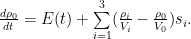
So this post will flesh the answer out by observing that the response defined by the “Bern TAR” parameters is simply the solution to the following equation:

where

But that equation describes the system that the accompanying diagram depicts. And that system does not impose partitioning of the type that the above-cited post describes.

In the depicted system, four vessels of respective fixed volumes 


Additionally, a gas source can add gas to the first vessel at a rate 

If appropriate selections are made for the 
The gas represents carbon (typically as a constituent of carbon dioxide, cellulose, etc.), the first vessel represents the atmosphere, the other vessels represent other parts of the carbon cycle, the membranes represent processes such as photosynthesis, absorption, and respiration, and the stimulus 
I digress here to draw attention to the fact that I’ve just moved the pea. The flow from the source does not represent all emissions, or even all anthropogenic emissions. It represents the flow only of carbon that had previously been sequestered for geological periods as, e.g., coal, and that is now being returned to the cycle of life. Thus re-defining the model’s emissions quantity finesses the objection some have made that the Bern Model requires either that processes (implausibly) distinguish between anthropogenic and natural carbon-dioxide molecules or that atmospheric carbon dioxide increase without limit.
Now, there’s a lot to criticize about the Bern Model; many of the criticisms can be found in the reader comments that followed the partitioning-argument post. Notable among those were richardscourtney’s . Also persuasive to me was Dr. Brown’s observation that the atmosphere holds too small a portion of the total carbon-cycle content for the 0.152 value assigned to the infinite-time-constant component to be correct. And much in Ferdinand Engelbeen’s oeuvre is no doubt relevant to the issue.
As the diagram shows, though, the left, atmosphere-representing vessel receives all the emissions, and it permits all of the other vessels to compete freely for its contents according to their respective membranes’ permeabilities. So what is not wrong with the model is that it requires the atmosphere to partition its contents, i.e., to withhold some of its contents from the faster processes so that the slower ones get the share that the model dictates.
Related articles
- On CO2 residence times: The chicken or the egg? (wattsupwiththat.com)
Surely if you want to model carbon dioxide properly you should identify the possible fates of it and develop equations which mirror those possible fate processes?
So, you have to suggest the following fates of newly emitted carbon dioxide:
1. Absorption into the oceans (affected by the oceanic temperature and the steady state phytoplankton population, as well as an minerals rate-limiting for phytoplankton growth (if any are indeed limiting)).
2. Absorption by land-based plants and photosynthesising micro-organisms (affected by the air temperature, the sunshine hours and the overall density of photosynthetic factories within land-based plants etc).
3. Absorption into rain and snow with subsequent deposition into soil, rivers or snow.
4. No fate at all.
The other question to consider is where the carbon dioxide gets emitted (human/animal-related emissions will be pretty much at land level, wild fires may see heat driving the gas up to greater altitudes, whereas volcanic eruptions may emit it a few miles into the sky) and whether that affects the rate of that carbon dioxide’s fate into one of those four pathways (dependent on atmospheric/stratospheric/tropospheric mixing to equilibrium).
Fancy maths is all very well, but a model which is related to real earth processes is likely to produce a better prognostic model than one which happens to fit past data for no reason better than mathematical chance.
I don’t know if it is possible to monitor carbon dioxide fate safely using methods distinct from radioisotope labelling, but if people want to understand the kinetics of carbon dioxide fate, they are going to need to develop just such methods in order to succeed in their mission. I’m assuming of course that no-one will let you go and realise a load of carbon-14-labelled gas into the atmosphere right now……..
All models are wrong. Some are useful. The carbon cycle equation in the Bern model is a mathematical approximation of a very complex progress. This approximation was first published in 1988 by Ernst Maier-Reimer and Klaus Hasselmann. It is used in many simple climate models.
The question is not whether it is a physical representation. It is not, and nobody in their right mind ever claimed it was. The question is whether it is a good approximation. It is, unless you want to explore the very distant future or very extreme scenarios. The definitive work on this is by Georg Hooss, who tried his best to break the model but could not.
Forgive my LaTeX blunder. The second equation should read .
.
Professors Pettersson, supported to some extent by Professor Brown, maintains that since the atmosphere at 600 PgC represents only 1.5% of the active carbon sinks (38,000 PgC in the hydroisphere and 2000 PgC in the biosphere) only 1.5% of any excess CO2 we add to the atmosphere will remain indefinitely.
The Bern model’s value for alpha-zero, on that analysis, is overstated by an order of magnitude,
with the implication that the later points on the curve, in particular, show too slow a rate of decay, leaving more excess CO2 lingering in the atmosphere to cause warming than is correct.
As I explained in my posting on this, it is in the equilibrium constant – the excess remaining indefinitely resident in the atmosphere – that the chief difference between the Bern model and the bomb-test curve is to be found. The thread unfortunately became derailed by those who wanted to argue about semantic definitions of relaxation and adjustment times – not the main point..
The bomb-test curve shows a decay towards the equilibrium constant 0.015 derived by Professor Pettersson from values for the contents of the atmosphere and of the active sinks given by IPCC (2007, 2013). It would be interesting if, on this thread, the semantic quibblers were to exercise a self-denying ordinance, for I should be interested in comments on whether the Bern model’s value of 0.152 for the equilibrium constant is justifiably an order of magnitude greater than that which is derivable theoretically from the relative magnitudes of the contents of the atmosphere and of the active sinks, and empirically from the bomb-test curve.
I only ask because I want to know. As a curious layman, I do not know which position is correct. But the discrepancy is large, potentially influential in climate terms and, therefore, interesting.
Richard,
What do you define as the very distant future? Is it 5 years, 50 years or 500 years or more?
What most non-chemists are either forgetting or not mentioning for non-scientific reasons is the Dalton’s law going back to 1800s where the total pressure of air is:
P(air) = P(N2) + P(O2) + P(CO2) + …..
Since contribution from N2 and O2 is 99% and from CO2 only 0.04% it means that out of 2500 molecules that contribute towards any property of air, only 1 molecule comes from CO2. So, whenever is someone arguing what 1 molecule of CO2 is doing, one has to explain what are 2500 molecules of N2 and O2 surrounding that molecule of CO2 doing at the same time!
Richard Tol: “The definitive work on this is by Georg Hooss, who tried his best to break the model but could not.”
Could you provide us a link and explain how his work supports, for instance, the high magnitudes for the infinite- and long-time constant components of the TAR impulse response?
Monckton of Brenchley: “Professors Pettersson, supported to some extent by Professor Brown, maintains that since the atmosphere at 600 PgC represents only 1.5% of the active carbon sinks (38,000 PgC in the hydroisphere and 2000 PgC in the biosphere) only 1.5% of any excess CO2 we add to the atmosphere will remain indefinitely.”
To this layman that reasoning makes sense and militates against the Bern TAR parameters. It probably should be mentioned, though, that Professor Pettersson’s equation is equivalent to the first Bern equation above if n = 1 and f_CO2_0 is 0.015.
@terry
500+ years
@Joe
http://www.schoepfung-und-wandel.de/NICCS/docum/welcome.html
“So what is not wrong with the model is that it requires the atmosphere to partition its contents, i.e., to withhold some of its contents from the faster processes so that the slower ones get the share that the model dictates.”
I agree with that. I think a simpler way of putting it is that some sinks are layered. The slow ones fill not from the air, but from the sinks above.
The model is empirical. It’s true that we don’t have long enough observation to accurately measure a 171 year time number. But we can use that to describe the long term behaviour, acknowledging that a timestep of 160 years, with appropriate parameter, would probably also have done well. And the component said to remain indefinitely simply reflects time scales too long to estimate at all. As Richard Tol says, it’s a model that works within a prescribed range.
Mathematically, a sum of exponentials is very hard to fit uniquely, because they are not at all orthogonal. It is an ill-conditioned problem. But all that means is that the Bern model is just one of many that can describe the process.
The empirical data show that Ao, the proportion of CO2 that remains in the atmosphere indefinitely must be very slightly less than zero. “Slugs” of CO2 are continuously being injected into the atmosphere by volcanoes, but the trend in CO2 in the atmosphere has been inexorably downward for the last 35 million years.
tty makes an interesting point I’d like to see comments on.
tty says: December 2, 2013 at 3:19 am
“The empirical data show that Ao, the proportion of CO2 that remains in the atmosphere indefinitely…”
It isn’t the proportion that remains in air indefinitely. It’s the proportion that remains so long that we can’t, in our limited observation span, measure the decay rate. The Bern model doesn’t claim to work for millennia. Here is an article from the originators in which they quote an expected range of 1765-2300 AD.
In answer to Roy Spencer, one should have regard to the various timescales to which the word “indefinitely” is applied. In the Neoproterozoic era, 750 Ma ago (Roy is too young to remember), there was at least 30% CO2 in the atmosphere. The CO2 was taken up in the oceans first as dolomitic limestone, then as amagnesic limestone, then as gypsum. During this phase, the equilibrium constant was demonstrably negative..
Now we are down to Henry’s Law, to the calcifying organisms, and to the growing net primary productivity of plants. In today’s geological conditions, therefore, the equilibrium constant may well be positive: and, if Professor Pettersson is right that it is the ratio of the carbon content of the atmosphere to that of the active sinks in the hydrosphere and biosphere, it is indeed slightly positive.
One problem with Professor Pettersson’s definition of the equilibrium constant is that, contrary to the geological evidence that it was for many ages negative, it can never be negative, for there cannot be a negative quantity of CO2 in the atmosphere. Another problem is that when the atmospheric partial pressure of CO2 doubles, the equilibrium “constant” also doubles by definition, and does so on a timescale of as little as a century.
I am beginning to wonder whether we have the slightest idea what the equilibrium constant is under today’s conditions. One cannot be sure that it remains negative. Equally, one cannot be sure that it is positive, still less that it is as strongly positive as the Bern model pretends. In this as in many other respects, the models are assuming that which cannot yet be known. What a relief it is, then, that The Science Is Settled, and we need not look any further into these matters.
tty: “‘Slugs’ of CO2 are continuously being injected into the atmosphere by volcanoes, but the trend in CO2 in the atmosphere has been inexorably downward for the last 35 million years.”
According to the attempt I made above to make sense of the Bern Model, tty’s statement would be a correct characterization of volcanoes’ actions if they are indeed introducing into the carbon cycle some carbon that for eons has not been participating.
To include the decay of which tty speaks, one or more of the vessels in the above diagram would need to be provided a second membrane, through which the gas would be consigned to the exterior darkness. Those membranes’ permeabilities (flow conductances) would need to be exceedingly small, of course.
tty is right to a point.
tty, adding a slug of co2 all things being equal cant reduce CO2 but all things being equal, but you’d intuitively expect that after the slug, given the emission and uptake remain constant at the level before the slug, that the CO2 would return over time to some equilibrium about the same as before the slug were added.
Despite Lord Moncktons plea, this problem is stated wrongly and assumes that uptake is a fixed function of time – but it is not, it’s a variable function of time, temperature, and CO2 concentrations at the places of major sinking activity.
The Bern model may be correct but it represents only a fraction of the system, a very simple model with no dynamic reactivity. We know for a fact that slugs of CO2 do not leave a large residual because despite the biosphere emitting slugs of CO2 constantly, CO2 has been known to contract.
The bomb test shows the turnover of CO2 due to all causes dynamic and static is on average more than this, but still misses the point that the response to a slug of extra CO2 may be much faster than the average drawdown if photosynthesis grows quickly with CO2 concentration, that is, if the sinks are being rate limited by the low concentration of CO2, if the sinking of CO2 is rate limited, then it will be harder to push up concentration, since the negative feedback is large, and any excess is rapidly acted against by the system,
The bomb test curve gives the decay rate of sink operating at an average rate between maybe 320 PPM and 400 PPM but how have the sinks actually responded, to that increase, the difference between the Bern model and the Bomb test may well be that factor. So how does that extra sinking capacity play out if we were to stop producing extra CO2 IE keep CO2 emission constant. That would depend on the dynamics of the feedback system that is rate limiting the sinks, and I might add the random effects of temperature on the biosphere. One must also consider the possibility that random pertubations have a bias, since the atmosphere is clearly biassed to reducing CO2 then random temperature changes are likely to be biassed to reducing CO2 over the long term.
For example, temp rises, oceans outgas, photosynthesis takes up ocean emissions limiting final CO2 level, temps fall, CO2 absorbed by oceans, CO2 now lower than it began.
Richard Tol: Thank you for the link. I assume you meant the dissertation to which that page in turn linked, i.e., to http://www.schoepfung-und-wandel.de/NICCS/docum/mpi_examen_83.pdf?
As to the software to which you did link, I’m flattered by the implication that I may be able to comprehend the nonlinear-system responses to which it is directed, but I must confess to skepticism that I will be enlightened.
Perhaps you could provide an executive summary of how you think that work supports the significant long-time-constant residues that the Bern TAR parameters dictate for the (linear) Bern Model.
tty
If I understand your point then a0 term seems ludicrous. If true then this would suggest CO2 would rise indefinitely given “additional” CO2.
But this excludes fluxes in the carbon cycle. As Lord Monckton has alluded to. Geochemical sequestration happens all the time via biological activity => carbonate minerals (for clarity this excludes sulphates such as gypsum which often precipitate in the same environment). As part of the rock cycle volcanic input is balanced by subduction of carbonate minerals in rocks such as limestone at destructive continental plate margins; this produces the volcanoes. In short the volcanoes are returning the CO2 from the subducted rocks. Interestingly, the d13 signature may vary from volcanos depending on whether the subducted rocks are biogenic or chemical in origin.
Lord M
One more appeal, let me use an electrical analogy, the bomb test gives us a hint as to the rate of sinking of energy. For an amplifier it’s akin to the average power sunk in the load. But does the power sunk in the load due to the dc biasing of the amplifier, give us any information about the gain of the amplifier? A small change in the conditions, may lead to a great change in output or a small one depending on the feedback acting. What are the feedback assumptiins in the bern model?
Instead of focussing on averaging a rate of sinking, I think we also need to use the bomb test to infer how the sinking rate has changed between the 1960s and now.
bobl: “We know for a fact that slugs of CO2 do not leave a large residual because despite the biosphere emitting slugs of CO2 constantly, CO2 has been known to contract”
In the diagram above, the CO2 emitted by the biosphere is represented by the leftward component of the net flow throw the membranes. Although this is something about which the model is silent, I would think of the net flow as a small difference between large leftward and rightward components. It is the sizes of those components–regarding which, again, the model is silent–that determines the rate of excess-carbon-14-concentration decay.
richardscourtney says: And the third model assumes that the carbon cycle is dominated by biological effects.
Looking at the annual changes in the amount of added CO2 to the atmosphere only this model makes sense.
It is worth noting that a large part of our emissions is absorbed by natural sinks. With this we agree everyone. From this it follows an important conclusion: natural sinks always react big increase on any new source. Natural sinks are not (almost) constants – there are (almost) in the balance with natural sources. The appearance of a new source always causes increase in productivity of sinks. Changes can not be linear.
How to react to organic of sinks – NPP, and decomposition (RH) on temperature changes?
Image 12 i 14 by M. Salby (http://wattsupwiththat.com/2013/11/22/excerpts-from-salbys-slide-show/) – here are the most important. They show – explained, that on the rapid changes in temperature RH reacts violently, and NPP (initially – and this is most important) responds slowly – much more slowly than RH. Land RH – respiration – responds rapidly to changes in temperature (rapidly – along with the temperature increase or decrease – much faster – more rapidly than NPP).
Therefore, I propose the following equation: “The Lotka–Volterra equations – models, also known as the predator–prey equations, are a pair of first-order, non-linear, differential equations frequently used to describe the dynamics of biological systems in which two species interact, one as a predator and the other as prey. The populations change through time according to the pair of equations”:
dx/dt = x (a -by)
dy/dt = – y (g-Sx)
where,
– x is the number of prey (for example, CO2 …);
– y is the number of some predator (for example, terrestrial plants …);
– dx/dt and dy/dt represent the growth rates of the two populations over time;
– t represents time; and
– a, b, g and S are parameters describing the interaction of the two, ie: where CO2 is the victim of a land photosynthesis is … predator.
Only by means of this equation we can prove that 4/5 – 5/6 (richardscourtney) added to the atmosphere of CO2 (presently) derived from natural sources. (http://climatechangescience.ornl.gov/content/historical-variations-terrestrial-biospheric-carbon-storage) : “Historical climatic variations which favored NPP over RH may have led to increased ecosystem carbon storage and might account for at least part of the “missing” sink required to balance the current century’s global carbon budget.”
When, however, the following: “NPP favored over RH”?
The higher density “prey” is easier, faster “hunting” …
Furthermore, according to the equation – model LV first grows RH, only when the NPP eg: produce seeds and produce new plants, it will be “favored NPP over RH” (http://en.wikipedia.org/wiki/File:Cheetah_Baboon_LV.jpg).
In the past it was. Sinks always coped with a much larger source of CO2. Never there have to saturation of sources. Always source increased.
Model Bern has a problem with sinks:
„It has been suggested that subtle and systematic changes in the net carbon fluxes as the result of climate variations or rising CO 2 concentrations over the past century may account for a substantial portion of the “missing” carbon sink of approximately 1 to 2 Gt C yr -1 needed to balance the contemporary atmospheric CO 2 budget.” (http://cdiac.esd.ornl.gov/pns/doers/doer34/doer34.htm)
NPP – in theory – be calculated as g C m-2 yr-1. Firstly, however, primarily calculated (or only) plant weight, and on this basis only estimated: g m-2 C-1 yr. In practice, not take into account the “nuances” such as: increase in CO2 = increase C concentration in plants: http://www.nature.com/scitable/knowledge/library/effects-of-rising-atmospheric-concentrations-of-carbon-13254108:
“The availability of additional photosynthate enables most plants to grow faster under elevated CO2, with dry matter production in FACE experiments being increased on average by 17% for the aboveground, and more than 30% for the belowground, portions of plants (Ainsworth & Long 2005; de Graaff et al. 2006). This increased growth is also reflected in the harvestable yield of crops, with wheat, rice and soybean all showing increases in yield of 12–14% under elevated CO2 in FACE experiments (Ainsworth 2008; Long et al. 2006).
Elevated CO2 also leads to changes in the chemical composition of plant tissues. Due to increased photosynthetic activity, leaf nonstructural carbohydrates (sugars and starches) per unit leaf area increase on average by 30–40% under FACE elevated CO2 (Ainsworth 2008; Ainsworth & Long 2005). Leaf nitrogen concentrations in plant tissues typically decrease in FACE under elevated CO2, with nitrogen per unit leaf mass decreasing on average by 13% (Ainsworth & Long 2005).”
Sorry by long quote…
Without a change in weight, the plants are able to accumulate many times more C than we think (and we are able to estimate by satellite). Tomatoes fertilized with CO2 – repeatedly increase the concentration of sugars in their juice and starch in the chloroplast – no mass change. In addition, NPP is not an important reservoir of C. This “tool” for the production of “remainders”. Them warmer (and more atm. CO2), but the more and faster (!), photosynthetic biosphere produces “remainders” (and these are the real “missing” sink) and .. decomposition “remainders” we are unable to (obviously good enough) estimated using satellites …. These are not “subtle” changes!
Conclusion: NPP can be removed from the cycle much more C than estimates CDIAC, the IPCC model Bern … “Missing” sink can be much larger than we expected.
Therefore: an increase in natural sources of C (XX century to today) can thus be large – larger than the size of our emissions.
… but of course we have to prove that Ferdinand Engelbeen is completely wrong here:
“… the 14C content of fossil fuel is zero: too old for 14C, which is below detection limit after ~60,000 years, while recent organics have recent levels of 14C incorporated. – the oxygen balance.”
That means that only humans are responsible for the δ13C decline , as the biosphere is not the cause and all other known sources are (too) high in δ13C.”
We must to prove that natural sources of old carbon increase during the twentieth century – supplemented a “small” carbon cycle. Trend of their increase was strongly positive. And I can try prove it.
… that if was not this increase (it according to L-V model) our C would not be added to the atmosphere …
I must also add that most of the subducted rocks are the denser ocean crust but sedimentary rocks also get subducted.
The input of CO2 into the system is about 0.3 GtC annualy, from volcanic sources.
This would replace the pre-industrial 535 GtC in only 1,800 years and completely turnover all the carbon in the biosphere in 135,000 years. The 800 Ky ice core data shows that CO2 varies between 240-300 ppm during this period, so it is reasonable to conclude that some process mineralizes carbon rapidly when atmospheric CO2 is high and mineralizes it more slowly when atmospheric CO2 is low.
Your three box model also ignores the fact that to interrogate the deep ocean, atmospheric CO2 must first interact with the surface layer; there is no direct route.
This was my simplistic three box model
http://i179.photobucket.com/albums/w318/DocMartyn/reseviours_zps4776b7df.png
cd: “As Lord Monckton has alluded to. Geochemical sequestration happens all the time via biological activity => carbonate minerals (for clarity this excludes sulphates such as gypsum which often precipitate in the same environment).”
Quite right. And you thereby touch on something I had initially thought to point out in the post but omitted because it would serve to distract unnecessarily from the point of the post. Specifically, my use of “carbon cycle” above is squishy; in effect I use it to refer to cycling through the atmosphere that occurs on time scales of less than a few centuries.
Hardly a bright line, I know, and probably inconsistent with more-conventional uses of the phrase. But I don’t think that detracts from the post’s main point, which is that the Bern Model does not require atmospheric partitioning.
DocMartyn: “Your three box model also ignores the fact that to interrogate the deep ocean, atmospheric CO2 must first interact with the surface layer; there is no direct route.”
Indeed. Moreover, the (actually, four-box) model shown there is not the only one that the Bern TAR parameters define; there no doubt are some that incorporate an indirect route. I have verified that for a system in which all four vessels are in series, for instance. And, although I don’t quite understand your model, but it likely can be characterized by the first Bern equation above.
– – – – – – – –
And the BERN modelers explained that time constant how?
(a why question is pending)
John
Monckton of Brenchley: “I should be interested in comments on whether the Bern model’s value of 0.152 for the equilibrium constant is justifiably an order of magnitude greater than that which is derivable theoretically from the relative magnitudes of the contents of the atmosphere and of the active sinks,”
I haven’t done the math. In fact, I can’t put my hands on the data I’d need for the attempt. But my guess is that some fitting of the n = 3 version of the first equation above to the data could indeed spit out parameters like the Bern TAR numbers–or not. But my understanding of Willis Eschenbach’s work is that the magnitude of the residuals thereby obtained would not be much less than that which results from fitting to a single exponential decay.
Mr. Tol seems to be in possession of knowledge that would refute the conclusion thereby to be drawn, but so far on this thread he has hidden his light under a bushel.
Joe
I was really only answering the call by Dr Spencer to address tty’s comment.
The partitioning does seem a little peculiar and seems to assume some intelligence in the system. I think that the d13C signature may play a part though. If the atmosphere becomes enriched with 12C then biological uptake may be more rapid thus removing the extra CO2 (if depleted in 13C) more rapidly than say the inorganic processes. This then acts in a feedback loop until things stabilise? Perhaps this is the reason why they feel some partitioning is required.
Nick Stokes-
“Mathematically, a sum of exponentials is very hard to fit uniquely, because they are not at all orthogonal.”
Are you claiming that Fourier series are flawed? Surely not.
Perhaps the problem is not with a long term residual concentration, but the assumption that this residual has something to do with past history. The biosystem has its own central tendency whatever we or volcanoes do. To explain this requires an additional term in the model that is separate from the time dependent terms.
John Whitman: “And the BERN modelers explained that time constant how?”
I’m putting words in their mouths here, but I think they’d say they’re not trying to explain anything but rather saying that, if you want to treat the system as a black box characterized by a linear differential equation, what equation of order n + 1 would you come up with if you fitted it to the data.
One criticism of their result is given in my last response above to Lord M. It is based on work that I thought I remembered Willis Eschenbach’s having done, but I haven’t been able to locate that work again. (His post I referred to above isn’t it.)
I agree with Nick Stokes’ comment on the difficulty of fitting multiple exponentials to decay curves. They are classically ill-conditioned and may result in very large errors.
Since there is a considerable biological component in CO2 uptake and release, is this likely to be a linear process? (I realse that with the available data this might be impossible to establish).
cd says
” As part of the rock cycle volcanic input is balanced by subduction of carbonate minerals in rocks such as limestone at destructive continental plate margins; this produces the volcanoes. In short the volcanoes are returning the CO2 from the subducted rocks.”
Certainly, though some of the CO2 may also be from deep mantle sources, or entrained from carbonate rocks through which the magma rises. And the whole cycle: atmospheric CO2 -> oceanic CO2 -> marine organisms -> carbonate deposit on seabottom -> move to a subduction zone by plate tectonics -> subduct to a depth where magma forms -> magma rises to the surface -> magma degasses -> atmospheric CO2 probably takes a few hundred million years at the very least. And it is far from clear that it is a balanced process. Since atmospheric CO2 on the whole seems to have decreased during the Phanerozoic indications are that it is not.
Doc Martyn says:
“The 800 Ky ice core data shows that CO2 varies between 240-300 ppm during this period, so it is reasonable to conclude that some process mineralizes carbon rapidly when atmospheric CO2 is high and mineralizes it more slowly when atmospheric CO2 is low.”
Its more like 170-300 ppm, and since the concentration tracks the glacial cycles fairly closely, with some lag (short during deglaciations, much longer during glacier growth phases) it would seem that the oceans are the only sink that could vary fast enough (on a time-scale of a few millenia). However I have no explanation why oceanic outgassing would lag rising temperature less than accumulation lags sinking temperatures.
The phrase “bern model” prodded my mmeory of having read an article by Jarl Ahlbeck a decade or so ago where he put forward a chemical mass balance model for the uptake of carbon dioxide by the oceans and biosphere, and then used it to predict the a size of around 17 GtC/year CO2 ocean/biosphere sink when the magic double of 560 ppmV concetration of CO2 in the atmosphere would happen instead of 8.5 GtC/yr (fro, The Bern Model I assume). He did this a little before the millennial shift and therefore had had only acess to data up to the year 1997 available estimate his parameters, but it should be check If his model has been tracking reality since then, or if we are really living inside the big bear bottles the author says the IPCC-(bern???)model thinks.
The article can be found at this URL.
http://www.john-daly.com/co2-conc/ahl-co2.htm
Joe,


 .
.
Your equations for the pressure in each box are incorrect given your compartment box model. This is a system of coupled first order linear differential equations that must be solved by an approach such as that described here: http://web.ist.utl.pt/berberan/data/40.pdf.
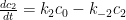
For the given system, an acceptable system of equations can written as follows (where c represents the molar concentration of the species of interest in the ith compartment):
subject to the chemical thermodynamic equilibrium constraint (i.e. equilibrium constant or partition coefficient relation):
Richard Tol:
George Box’s aphorism that “All models are wrong.” is obviously incorrect in reference to the natural laws. Until recently, it was correct in reference to models of complex systems such as the climate. Today, however, through the use of modern information theory, it is possible to build a model of a complex system that conforms to the principles of reasoning, thus not being wrong. All currently available climatological models are, however, wrong.
Fun stuff ladies and gentlemen.
Chaucer ably described the dominant factor in Earth`s carbon balance, as follows:
WHAN that Aprille with his shoures soote
The droghte of Marche hath perced to the roote,
And bathed every veyne in swich licour,
Of which vertu engendred is the flour…
We now have the benefit of the beautiful AIRS data animation of atmospheric CO2 at
http://svs.gsfc.nasa.gov/vis/a000000/a003500/a003562/carbonDioxideSequence2002_2008_at15fps.mp4
The CO2 seasonal sawtooth is dominated by the larger Northern Hemispheric (“NH“) landmass.
Atmospheric CO2 drops in NH Spring and Summer during Chaucer’s “shoures soote” as photosynthesis dominates, and then CO2 increases in NH Fall and Winter as oxidation becomes the dominating factor in this huge and wondrous equation.
The annual amplitude (from memory) of this magnificent seasonal CO2 sawtooth is about 16-18ppm in the far North (measured at Barrow AK), and as little as 1-2 ppm at the South Pole.
Nevertheless the average upward slope of the “global” (approx. equal to Mauna Loa) CO2 sawtooth is about 1-2 ppm per year. Aye, there`s the rub!
And some of us think we understand why CO2 increases (for example, the Mass Balance Argument attributes the CO2 increase to fossil fuel combustion), while Richard Courtney ably suggests that we don`t really know. I`m generally with Richard on this, although I wobble.
There are days when I think the Mass Balance Argument (`MBA`) has validity, although I suggest that other factors such as deforestation etc. may play a larger role, and it is not just fossil fuels.
Then there are other days when I think the MBA is overly simplistic. The limited data I have seen suggests that even in urban environments where fossil fuels are locally combusted, the daily CO2 signature is overwhelmingly natural. It appears that CO2 is sufficiently scarce that plants quickly gobble up excess CO2 close to the source. Yum!
In any case, the global CO2 Balance question is very interesting, but I suggest it is not that relevant to the oft-fractious global warming debate – because CO2 in Earth`s natural system is clearly driven by temperature and is at most an insignificant driver of temperature.
Some people insist that these matters must be quantified, so I will accommodate them:
The impact of the current increase in atmospheric CO2 on Earth temperature is less than one Standard Farticane*.
Regards to all, Allan
******
* 1 Standard Farticane = I Fart in a Hurricane, at Standard Temperature and Pressure.
CD:
“As part of the rock cycle volcanic input is balanced by subduction of carbonate minerals in rocks such as limestone at destructive continental plate margins; this produces the volcanoes. In short the volcanoes are returning the CO2 from the subducted rocks.”
<<<<<<<<<<<<<<<<<<>>>>>>>>>>>>>>>>>>
Not all volcanoes return subducted material. Some occur at spreading centers, others at “hot spots”, i.e., Hawaian Islands, and such do not return subducted material but tap directly into the mantle. So carbon is not being recycled but added to the crust or atmosphere, insofar as such volcanoes produce CO2. However, subducted material is recycled by those volcanoes that occur on the margins of subduction zones, as you say.
rtj1211 says: “I’m assuming of course that no-one will let you go and realise a load of carbon-14-labelled gas into the atmosphere right now……..”
Good news! Iran intends to go ahead with this experiment within the next ten years.
Allan MacRae says: “The CO2 seasonal sawtooth is dominated by the larger Northern Hemispheric (“NH“) landmass.”
Or is it dominated by the larger Southern Hemisphere (“SH”) oceanic surface area?
ZP: “Your equations for the pressure in each box are incorrect given your compartment box model. ”
Could you be a little more specific? The equations you wrote are not inconsistent with mine, except E in my system is a rate of mass flow, so I would have put E in your equations instead of dE/dt. Also, for parallelism I perhaps confusingly use rho to represent the mass (number of moles) in the vessels; it’s not a concentration. Other than that, your k’s are my S/V’s.
In short, you’ve told me the equations are wrong, but you haven’t pointed out where. I’d love to have someone vet my sums, but I’ll need a little more specificity if it is to do me any good.
DocMartyn: “Your three box model also ignores the fact that to interrogate the deep ocean, atmospheric CO2 must first interact with the surface layer; there is no direct route.”
That’s incorrect. There is significant up-welling of deep waters in certain ocean regions, esp. Indian Ocean and sinks at the poles. This is part of the thermohaline circulation. That provides a direct connection.
http://climategrog.wordpress.com/?attachment_id=715
The point you try to make may well apply to mid-ocean waters between the surface mixed layer and the thermocline.
I am writing up something that shows that the well-mixed layer has a time constant close to one year and equilibrates in under a decade with a change of the order of 10ppmv/K. The circa 15y ( Bern 18.6y ) time constant is presumably this mid level diffusion.
Lance Wallace fitted a time const of 1.17 years to Nordrap C14 data in an earlier discussion. This is close to what I’m finding by totally different methods that does not suffer from the lack of uniqueness described here for exponentials.
Gosta Pettersson is close to being correct in his conclusions but I think his working is wrong. He sees no need for the short period which IMO he should be applying to his El Nino changes.
He has recently pulled his papers 1 & 2 which he is rewriting them, so it will be interesting to see how he changes them.
me says: “with a change of the order of 10ppmv/K.”
That is atm 10ppmv. I view of the volume ratio, I would guess about 4x that for the mid-level reservoir giving total all the order of 50 ppmv/K. This is in rough agreement with Gosta’s figures by via a different (incompatible) calculation.
The resulting conclusion is the same w.r.t. solving the “missing sinks” issue: like the missing heat, it does not exist.
The k’s in the equations represent the specific rate constants governing the compartmental exchange rates. Your equations incorrectly assume that the forward rate constant ( ) is equal to the reverse rate constant (
 ), which allowed you to factor them out as a single constant S. There is no physical basis on which to assume that the forward rate constant should be equal to the reverse rate constant. And, the values will only be the same in the case where the equilibrium constant is unitary.
regarding the comment by tty:
Since the late Eocene, the world has cooled considerably which must mean cooler oceans and a greater capacity for holding CO2, presumably. But, in terms of geologic time, the carbon equation must be incalculable.
For example, carbonates are precipitated directly from ocean waters at such places as the Bahamas or the Yucatan shelf, such areas being known as carbonate platforms. Thus carbon is removed on a semi-permanent basis at such places. An ocean richer in CO2 would positively affect the rate of precipitation, presumably. I doubt that all these factors can be untangled.
jorgekafkazar says:
Allan MacRae says: “The CO2 seasonal sawtooth is dominated by the larger Northern Hemispheric (“NH“) landmass.”
Or is it dominated by the larger Southern Hemisphere (“SH”) oceanic surface area?
Yes, indeed. Yet another urban climatology assumption I guess.
Annual ‘saw tooth’ works out rather nicely actually since it can be modelled by two ramps or 12moand 6mo cosines (the latter being more physically real, but the first is handy for getting flow rates).
http://climategrog.wordpress.com/?attachment_id=721
The Bern model can be thought of as a partition of reservoirs, but that is only an approximation. Generally, such “long tailed” models arise from partial differential diffusion equations. The sum of exponentials is an expansion of eigenfunctions of the partial differential equation.
So, the place to begin is the PDE model, the equations and their boundary conditions, assumed by the Bern model.
Subduction is not required. Folding deposits deep enough for metamorphosis is sufficient to release CO2.
The CO2 sources for many of the ‘hot spot’ volcanoes, e.g., Hawaii, are unknown. Guesses about magma absorbing CO2 from sediments as magma passing through are just that, guesses.
Deep, really deep magmatic CO2 sources, are currently beyond our ken. CO2 out gassing from these hot spots may include primal CO2 still leaking from earth’ s core. Carbon content in metals often resides in carbides; oxygen in many forms, oxides to be simple. Bluntly speaking, carbon is abundant cosmically.
ZP: “here is no physical basis on which to assume that the forward rate constant should be equal to the reverse rate constant.”
If you’re talking about the real world, in which various factors affect “natural” emission (leftward flow) and uptake (rightward flow), I agree, and to that extent the model does not reflect reality.
If you’re talking about the model world, in which a permeable membrane conducts net flow in accordance with the pressure difference–i.e., with the difference in moles/unit volume, then I’m free to assume that a pressure on one side causes the same flow as the same pressure on the other.
The concept of equilibrium constant may be causing the difficulty here. Note that the process so drives flows that vessel contents tend toward proportionality with their volumes V. That’s where the equilibrium constants come from.
Bart: “So, the place to begin is the PDE model, the equations and their boundary conditions, assumed by the Bern model.”
No. The Bern equations are exact solutions to ordinary differential equations. The equation that results from plugging the Bern TAR numbers into the first equation above is an exact (except for computation rounding) solution to the third equation above, which is not a partial differential equation.
No doubt some diffusion does occur in the real-world carbon cycle, but the Bern model does not reflect that.
Joe, I think Bart’s comment was intended to mean that a diffusion model produces somthing very similar to the ‘long tailed’ triple exp. model. Not that is was mathematically identical.
IIRC either Nick Stokes, or WHT has worked out a three slab ocean diffusion model that essentially comes out the same.
Greg Goodman: “[A] diffusion model produces something very similar to the ‘long tailed’ triple exp. model.”
Indeed. If I remember correctly, I once computed seven or eight vessels in series (ODE) to approximate the “tautochrone” results I had obtained here http://wattsupwiththat.com/2012/07/13/of-simple-models-seasonal-lags-and-tautochrones/ through a diffusion equation (PDE).
Allan MacRae says: “The CO2 seasonal sawtooth is dominated by the larger Northern Hemispheric (“NH“) landmass.”
jorgekafkazar says on December 2, 2013 at 9:22 am
Or is it dominated by the larger Southern Hemisphere (“SH”) oceanic surface area?
Allan again:
Hi Jorge,
I suggest that it is as I said. Please examine the timing and direction of the atmospheric CO2 sawtooth (measured at Mauna Loa) superimposed in the AIRS animation, which I suggest is dominated by larger NH landmass photosynthesis.
But I am open to discussing your point. What natural mechanisms would support your hypo?
Best, Allan
[Actually Jorge I think your point is just wrong, but I’m trying to be polite.]
Joe Born says:
December 2, 2013 at 10:45 am
The equilibrium between two reservoirs is governed by the equilibrium constant for that process. Consider the equilibrium between in the atmosphere and
  in water (i.e. Henry’s law). That equilibrium is given by:

![K_{eq}=\frac{\left [ CO_{2} \right ]\left ( aq \right )}{\left [ CO_{2} \right ]\left ( g \right )}](https://s0.wp.com/latex.php?latex=K_%7Beq%7D%3D%5Cfrac%7B%5Cleft+%5B+CO_%7B2%7D+%5Cright+%5D%5Cleft+%28+aq+%5Cright+%29%7D%7B%5Cleft+%5B+CO_%7B2%7D+%5Cright+%5D%5Cleft+%28+g+%5Cright+%29%7D&bg=ffffff&fg=000&s=0&c=20201002)
such that the equilibrium constant for the process can be written as:
In this example, note that the equilibrium constant is not governed by the volume of the respective reservoirs. It is governed by the equilibrium molar concentration or (equivalently) partial pressure within each reservoir. The total mass contained within each reservoir at equilibrium will depend upon their respective volumes. However, chemical equilibrium is not defined in this manner (for more details refer to http://en.wikipedia.org/wiki/Chemical_equilibrium). Finally, the thermodynamics of the system dictate the form that the kinetic rate laws (differential equations) must take.
Allan MacRae says: “The CO2 seasonal sawtooth is dominated by the larger Northern Hemispheric (“NH“) landmass.”
jorgekafkazar says: Or is it dominated by the larger Southern Hemisphere (“SH”) oceanic surface area?
Greg Goodman says: December 2, 2013 at 10:30 am
Yes, indeed. Yet another urban climatology assumption I guess.
Annual ‘saw tooth’ works out rather nicely actually since it can be modelled by two ramps or 12mo and 6mo cosines (the latter being more physically real, but the first is handy for getting flow rates).
http://climategrog.wordpress.com/?attachment_id=721
Allan again:
Depends upon the year Greg, and whether Earth is warming, cooling or neither.
Annualized Mauna Loa dCO2/dt has “gone negative” a few times in the past (calculating dCO2/dt from monthly data, by taking CO2MonthX (year n+1) minus CO2MonthX (year n) to minimize the seasonal CO2 “sawtooth”.)
These 12-month periods are (Year-Month ending):
1959-8
1963-9
1964-5
1965-1
1965-5
1965-6
1971-4
1974-6
1974-8
1974-9
Has this not happened recently because of increased humanmade CO2 emissions, or because the world has, until recently, been getting warmer?
Mr. Born, thank you for taking the time to write this intriguing and highly useful post.
Now that you have acknowledged (at 11:15am) the accuracy of Greg Goodman’s clarification (at 11:01am) of Bart’s suggested path forward, how about now replying more meaningfully to Bart (at 10:41am)? This layperson is left (for now) with the impression (hopefully, mistaken) that you are intentionally avoiding discussing meaningfully Bart’s suggestion.
Your conscientious and polite responses above are wonderful. Well done.
I was just trying to point out where I think the expansion of the Bern model comes from, because I did not see anyone mention anything about diffusion processes above, and thought I might be able to clarify or elucidate how the model comes about. If what I suggested is already known by the participants, then never mind.
Obviously, the Bern model is chock full of assumptions which, based on observations, appear to be wrong in whole or in part. I’m not defending it by any stretch of the imagination.
ZP: “[T]he equilibrium constant is not governed by the volume of the respective reservoirs. It is governed by the equilibrium molar concentration or (equivalently) partial pressure within each reservoir.”
In this case equilibrium is equal molar concentrations. There are no chemical effects biasing the system. The partial pressure (in the case, the complete pressure) is proportional to the molar concentration and is, as I indicated above, rho / V.
Janice Moore: “This layperson is left (for now) with the impression (hopefully, mistaken) that you are intentionally avoiding discussing meaningfully Bart’s suggestion.”
Actually, I did address his comment.
Diffusion, which he’s talking about, can be thought of as a situation in which an infinite number of infinitesimally small vessels are connected in series. The solution can be thought of as an infinite sum of infinitesimal exponentials, but it is expressed in other terms, such as error functions.
That’s not what the Bern equation is. Since the Bern solution is a finite number of exponentials, it is the solution to a linear ordinary differential equation. If the parameters are right, the result can look a lot like the solution to a diffusion (a type of partial-differential) equation, so, as Mr. Goodman pointed out, one could in the right circumstances look upon it as an approximation to a diffusion-equation solution.
But the Bern equation is an exact solution to what I’ve heard adepts in this discipline refer to instead as a “lumped-parameter” equation, which describes the diagram I provided above.
Hi Allan, good to have you on board.
In relation to your paper on phase relationships I suggest you read my recent article on Climate Etc. re. running means. It does not negate what you found but could help improve it.
http://judithcurry.com/2013/11/22/data-corruption-by-running-mean-smoothers/
“Annualized Mauna Loa dCO2/dt has “gone negative” a few times in the past ”
I have little time for this kind of climatology home spun data distortion techniques. It seems that by “annualised” you mean some kind of “anomaly” calculation. If you wish to remove annual and sub-annual cycles use an appropriate filter (unless you absolutely need to look at the last year or two of data).
Yes, 1974 was a low point but did not go negative in this plot. Why would it matter if it did?
http://climategrog.wordpress.com/?attachment_id=720
Clearly there are a number of factors at work, not just one simple relaxation process driven by temperature. Indeed , since 1995 and start of the “plateau”, it seems that AO correlates better than SST. This is also a reflection of Henry’s Law
. http://climategrog.wordpress.com/?attachment_id=259
All that is ignoring the non negligible question of data sample errors and “bias corrections”.
None of this is simple but we’re guessing for some first order approximations. Don’t be surprised is some years deviate. Does not disprove a hypothesis.
Joe Born says: in water. As shown in this table http://en.wikipedia.org/wiki/Henry's_law#Other_forms_of_Henry.27s_law, the equilibrium constant for the solubility of
  in water at 25 °C is
  M/atm (which is considerably different than 1).
December 2, 2013 at 12:25 pm
In this case equilibrium is equal molar concentrations. There are no chemical effects biasing the system.
Equilibrium being achieved at equal molar concentrations is not generally the case. Consider the solubility of
I agree with the nomenclature. However, the forward rate constant cannot be assumed equal to the reverse rate constant. This approach is contrary to known chemical thermodynamics of these systems. Chemical equilibrium is achieved when the forward rate equals the reverse rate (i.e. ) such that
  . So, the ratio of the forward rate constant
  to reverse rate constant
  must also equal the ratio of the equilibrium molar concentrations, which are measured values and normally are not equal (as exemplified above for the solubility of carbon dioxide in water).
Joe Born says:
December 2, 2013 at 12:40 pm
Not to stir a tempest in a teapot, but a lumped parameter model is generally a method for expressing a PDE system as an expansion in ODEs. So, while the Bern model is an exact solution to the set of ODEs describing the approximated system, it is an approximate solution for a much more complicated model.
As far as I can tell, the Bern models, for there appear to be more than one, are a distillation into ODEs of a sort of hybrid PDE/ODE model. For example, Bern-SAR is described by
Well, Mr. Born, thanks for acknowledging my concern, but, it is clear to me, at least, that you have not yet meaningfully addressed what Bart said. It appears that you do not realize what Bart is trying to say to you. There is definitely a communication break-down, there — I’m assuming it is not intentional.
And if this issue is, indeed, not essential (a “tempest in a teapot”), by all means ignore my pleas to address it.
http://climategrog.wordpress.com/?attachment_id=722
The Nordkap data , at least seems to support the idea of a short decay constant. (Though not as short as my SST/CO2 work is suggesting. This may related to NH/SH delay of transfer from strato to tropo delays.)
There seems to be some clear oscillation in the initial decade whose magnitude is at least close to the initial decay relationship.
this would seem to be ” consistent with” the idea of dilution of C14 ratio by the continual turn over between atm and mixed layer. After initial dilution and equilibration with mixed layer the longer (diffusion?) to second ocean slab takes over.
There are so many sinks and sources in all this that there may be a different physical interpretation but the above seems likely to me.
tty says:
December 2, 2013 at 3:19 am
The empirical data show that Ao, the proportion of CO2 that remains in the atmosphere indefinitely must be very slightly less than zero. “Slugs” of CO2 are continuously being injected into the atmosphere by volcanoes, but the trend in CO2 in the atmosphere has been inexorably downward for the last 35 million years.
The question of volcanic CO2 emissions is one that really is not well understood by any one. For instance, looking for information on the isotopic signature of volcanic CO2 leads to the fact that at present, there really isn’t any reliable generalization (http://www3.geosc.psu.edu/courses/Geosc518/15_Random_Mixing_Model/Chapter_15/Mantle%20Carbon.pdf).
In one view most, if not all, volcanic CO2 is “new” carbon as far as the biosphere is concerned. That is, volcanic emissions are mostly not reworked or naturally “recycled” biological carbon. It consists of carbon that has been driven off the core through fractionation and has been working its way to the surface through tectonic processes. The isotopic composition should reflect the composition of the nebula that planet condensed from during the formation of the solar system. There are also some arguments that the commonly used figures for volcanic carbon emission are far too low.
As the pdf above notes, mantle xenoliths can consist of crustal fragments subducted and reworked. This will be true only within the vicinity of active or extinct subduction zones. Mantle plumes such the one that drives the Hawaiian Island volcanoes, or Yellowstone are not linked to any known subduction processes.
As regards atmospheric CO2, the concentration trend has been “inexorably down” for about 150,000,000 years (roughly since the mid-Mesozoic).
Janice Moore: “It appears that you do not realize what Bart is trying to say to you.”
Perhaps. What I initially thought he meant was that the Bern model implies diffusion and that my diagram, which depicts a lumped-parameter system, not a distributed-parameter one, therefore does not depict a system to whose system equations the Bern equation is a solution.
What I now understand him to mean is that the reason why the authors of the Bern equation came up with a sum of exponentials was to approximate the solution to a diffusion equation. That’s conceivable, although I don’t know why they’d settle for an approximation when they could have used the exact solution. In any event, I no longer understand Bart to say that my diagram’s system equation has as its solution something other than the function that results from plugging the Bern TAR parameters into the Bern equation.
Therefore, since the Bern equation applies to that diagram, and since that diagram’s first, atmosphere-representing vessel does not partition its contents, my point stands that the Bern equation does not require (arguably implausible) partitioning, so it would be best not to base an argument against its use on its imposing such a requirement.
My review of the bidding is that no one so far has faulted my reasoning except ZP. His argument is that my diagram”s system equation is not what I think it is. If he were right, of course, that system equation’s solution, which I think is the Bern equation with the Bern TAR parameters plugged in, might not be. That would undermine my reasoning. But I think ZP knows a formula from chemistry but doesn’t really know when to apply it. I’m no scientist, but I have dealt with technical types extensively, and in my experience that type of error is not uncommon.
–Of course, I could be wrong.
ZP: “Equilibrium being achieved at equal molar concentrations is not generally the case. Consider the solubility of CO_{2} in water.”
I’ll grant you that equal concentrations at equilibrium are bot the case in all systems. I’m no scientist, but I did take high-school chemistry.
But will you grant me me that, in a situation in which you have two vessels containing the same, identical ideal gas and joined by a permeable membrane, the equilibrium condition may–just may–be equal pressures in the vessels?
And, even if you don’t, could you grant that if such a system were to exist, my equations describe it? Because the question before the house is whether the Bern equation requires the atmosphere to partition its CO2 contents implausibly, and, to the extent that my equations describe a system that doesn’t perform such partitioning, it demonstrates that the answer to the question is no.
Joe Born says:
December 2, 2013 at 2:38 pm
I’m not faulting anything. Just trying to facilitate understanding of how they arrived at the model. As to why they’d settle for an approximation, it would be to get a closed form solution in terms of elementary functions.
I fear I am only detracting from the conversation, though, which was the opposite of my intention. Pray carry on and consider it no further.
ATheoK says:
“Subduction is not required. Folding deposits deep enough for metamorphosis is sufficient to release CO2.”
True, but it requires rather extrene ultra-high-temperature metamorphism. Normally limestones and dolomites just turn to marble.
“The CO2 sources for many of the ‘hot spot’ volcanoes, e.g., Hawaii, are unknown. Guesses about magma absorbing CO2 from sediments as magma passing through are just that, guesses.”
Not really, we might not be able to see it happen in real time, but decarbonation by contact metamorphism is very well known and documented. As a matter of fact it is much more common than UHT metamorphism.
Sorry Joe, I’m just trying to help you with your post. It is apparent that you have a fundamental misunderstanding of chemical systems, since you do not appear to appreciate that fact that the forward and reverse rate constants will not generally be equal. ) is equal to the reverse constant ($latex k_{ma}) as indicated on page 176:
Perhaps an alternative argument for why your approach is incorrect would help. Your approach predicts that the equilibrium position between reservoirs will be essentially independent of temperature, because you are equating the forward and reverse rate constants. This is in direct conflict with known thermodynamics of chemical systems, such as the solubility of carbon dioxide in water (see http://en.wikipedia.org/wiki/Henry's_law#Temperature_dependence_of_the_Henry_constant). However, by recognizing that the forward and reverse rate constants are independent of each other and are each adequately described by the Arrhenius equation (http://en.wikipedia.org/wiki/Arrhenius_equation#Equation), you’ll be able to provide an excellent molecular dynamics explanation for this observation (see http://en.wikipedia.org/wiki/Transition_state_theory).
However, if this argument and the previous references I have provided do not help, hopefully, this paper, which discusses the Bern model, will: http://onlinelibrary.wiley.com/doi/10.1111/j.2153-3490.1975.tb01671.x/pdf. I’ll direct your attention to equation 1 on page 170. In this equation, the authors have introduced two rate constants that they refer to as exchange coefficients. The authors do not assume the forward constant (
Sure.
Joe, I’m hope you realize that I’m not defending the Bern model. I just want to help you formalize your arguments and objections in a manner that will be accepted by physical chemists. When you begin discussing the partitioning of , you immediately invoke the thought of partitioning between air and water, which is a chemical equilibrium phenomenon. As such, this situation is quite different from the simplistic two vessels joined by a permeable membrane that you appear to want to invoke.
ZP: “When you begin discussing the partitioning of CO_{2}, you immediately invoke the thought of partitioning between air and water, which is a chemical equilibrium phenomenon.”
I’m afraid we aren’t going to be able to join issue.
I’m telling you what the Bern mathematics says, not what happens in the real world or what the authors were shooting for when they wrote it. I agreed at the outset that the Bern equation does not reflect the the fact that emissions and uptake processes are asymmetrical and that it fails to that extent to reflect the real world. But with the Bern TAR parameters, the Bern equation expresses the solution to the differential equations that the system I illustrated dictate–with equal pressures at equilibrium.
What you say about equilibrium between CO2 in air and CO2 in water is no doubt true, but it’s irrelevant. Now, if you can show me that the Bern equation does not give the the solution to the diagrammed system as I’ve described it, with the symmetry I’ve assumed in writing the equations, then you’re addressing the subject of the post. Otherwise, I don’t think either of us will benefit from further discussion.
The argon in the Earths interior comes from radioactive decay and it would be nice to measure its release from volcanic sources, which would give us an good estimate of volcanic activity during the last 800 ky.
Look, the ranges of response vary between the dumb hindquartered sks kidz arguing that the isotope ratios alone implicate human CO2, and the elegant process engineering of Ferdinand coming to the same conclusion. It is utterly reasonable to suspect that when you dump a bunch of something in the system, and the system concentration of the something increases, the increment will be yours.
However, our contribution is small, and the system is poorly understood. Furthermore, we are feeding the biological cycle exactly what it needs. I argue we simply cannot know right now. The same applies to the so called e folding which is the notion that an exceptional slug of something the system is not prepared for will take longer to absorb. All well and good, but this notion calls into question a dozen factors we know even less about. Study large igneous provinces, and you may well suspect, as I do , that the human volcano is nothing unprecedented.
So what is not wrong with the model is that it requires the atmosphere to partition its contents, i.e., to withhold some of its contents from the faster processes so that the slower ones get the share that the model dictates.
+++++++++++
The problem I see is that every year the earth absorbs 1/2 of human emissions, and this amount is dependent upon human emissions, not total CO2 is the system, as this has been going on for many years.
now it is true that human beings have an infinite capacity to rationalize, so I’m sure there are as many different explanations for this are there are people. And every expert will have 2 explanations. However, to me it is a nonsense.
How can nature tell how much CO2 humans are producing each year, such that nature absorbs almost exactly 1/2 year of human emissions after year after year? How come nature doesn’t absorb the excess as a function of the total? How can nature separate human emissions from natural emissions?
This to me is the crux of the problem. Nature cannot tell human from natural emissions and thus what we observe is not what we believe it to be. The 1/2 figure has mislead us into believing facts not yet in evidence. the unknown is staring us in the face.
Nick Stokes: “The model is empirical. It’s true that we don’t have long enough observation to accurately measure a 171 year time number. ”
You do understand that the second sentence refutes the first sentence, right? If it is not based on observation — it is not empirical. Unless you want to wordsnitch the definition of ’empirical’ to be the same as ‘unempirical.’
tty: “However I have no explanation why oceanic outgassing would lag rising temperature less than accumulation lags sinking temperatures.”
How about this? Ocean outgassing in warm tropical and subtropical upwelling zones is intercepted more efficiently by microbial dark matter than in the polar downwelling brine rejection zones at -2C.
Greg Goodman says: December 2, 2013 at 12:45 pm
Sorry Greg – I do not accept your comments, and I do not want to pursue this discussion further.
If you want to critique, you have to first demonstrate that you understand what was said, and what was not said.
Allan MacRae says: “Sorry Greg – I do not accept your comments, and I do not want to pursue this discussion further.”
Allan, that is a very poor response to anything. if you want to refuse to accept my comments you need to first demonstrate that you have understood what they said.
I am in total agreement with the 9month lag and what it tells us about phase relationship. I have posted similar stuff myself and am working on something much more detailed which goes further. My comment here was merely that you are using a crap filter and your results may be clearer if you used a better one. (See my article on Judth Curry’s site for a detailed analysis and some ready made alternatives , with code !)
If you don’t think that running means distort data and are probably reducing the correlation that you are trying to demonstrate, please post a comment on Climate Etc. thread.
If you think I am criticising your article more than that you are mistaken. The dominant periodicity once the annual and sub-annual variation is removed is about 3 years, this is 4x9months thus the two are in quadrature.
Here is the clear alignment of dCO2 and SST using a lanczos filter.
http://climategrog.wordpress.com/?attachment_id=720
You will notice that the correlation is not so great in the detail beyond 2000. However, there is a remarkable correlation with a variable delay on Arctic Oscillation.
http://climategrog.wordpress.com/?attachment_id=259
Conclusion is that it is not trivially SST but it does account for a large amount of the variation.
PS. As Salby points out in his lecture, geological records show temp and CO2 correlate directly but with a substantial lag. That raises the question : on what time-scale does it flip from derivative to direct correlation?
I have an answer to that question that I am currently writing up and it is a little surprising.
jorgekafkazar says:
December 2, 2013 at 9:22 am
Or is it dominated by the larger Southern Hemisphere (“SH”) oceanic surface area?
It is easy to make the distinction: ocean CO2 releases are slightly increasing the δ13C level of the atmosphere, while CO2 releases from vegetation are firmly decreasing the δ13C level. Uptake by the oceans also slightly increases the δ13C level (because both ways are pure physical partitioning where the lightest isotope gets faster in/out, but the ocean surface is much higher in δ13C level than the atmosphere), while the uptake by plants (no matter C3 or C4) firmly increases the δ13C level. That gives in average for the past 22 years (CO2 and δ13C zeroed in January) :
http://www.ferdinand-engelbeen.be/klimaat/klim_img/seasonal_CO2_d13C_MLO_BRW.jpg
which shows that the variability over the seasons is completely dominated by the NH vegetation.
The trend also comes from the NH, as can be seen by comparing the trends over the years for different stations:
http://www.ferdinand-engelbeen.be/klimaat/klim_img/co2_trends_1995_2004.jpg
It takes time for the increase to reach altitudes and to pass the ITCZ from the NH to the SH.
Vegetation is not the cause of the increase, as the oxygen balance shows a small deficit, caused by increased growth.
The oceans are not the cause, as the most important upwelling places are in the SH equatorial Pacific, but the increase is in the NH first (and the δ13C trend is opposite to ocean releases).
Other possible natural sources are either too small or too slow…
So what is left?
“So what is left?”
Never the most convincing argument.
Your plot of relative timing is interesting.
http://www.ferdinand-engelbeen.be/klimaat/klim_img/co2_trends_1995_2004.jpg
Following your simple logic that this is the progression of the same signal (impossible to see in the integrated levels), it suggests that the increase starts in the Arctic , as indicated by Barrow station in Alaska.
Compare to my graph of d/dtCO2 (which does allow us to identify patterns) :
http://climategrog.wordpress.com/?attachment_id=259
It shows Arctic atm. pressure correlates with a strong lead.
Joe Born says:
In this case equilibrium is equal molar concentrations. There are no chemical effects biasing the system. The partial pressure (in the case, the complete pressure) is proportional to the molar concentration and is, as I indicated above, rho / V.
Sorry, a bit late in the discussion, as I was travelling…
There are huge chemical effects biasing the system, that is one of the basics of the Bern model. The three main sinks: ocean surface, deep oceans and vegetation all three are assumed to react with their own time constants, but also limitations in maximum uptake.
For the fastest, the ocean mixed layer, that is anyway certain: a 100% change in the atmosphere is followed by a 100% change of free CO2 in the ocean surface, as per Henry’s law, but as free CO2 in the ocean surface is only 1% of total carbon, the total carbon increases with ~10%, thanks to the chemical equilibria: 10 times more than for fresh water, but 10 times less than the change in the atmosphere.
That is the Revelle (or buffer) factor. Chemical equilibria explained in:
http://www.eng.warwick.ac.uk/staff/gpk/Teaching-undergrad/es427/Exam%200405%20Revision/Ocean-chemistry.pdf
Thus the Bern model assumes that the ocean surface rapidely is in equilibrium, but limited in capacity (I assume that the 19% is including the fast part of the biosphere besides the ocean surface). Which is theoretically and empirically proven. DIC (total inorganic carbon) increased about 10% of the atmospheric increase over the past decades as measured in Bermuda and Hawaii:
http://www.biogeosciences.net/9/2509/2012/bg-9-2509-2012.pdf
http://www.pnas.org/content/106/30/12235.full.pdf
The same for the deep oceans, but the deep oceans don’t show any sign of saturation, at least not for the foreseeable future, as the pCO2 of the cold sinking places is and remains very low, thus still increasing their uptake for increasing CO2 levels in the atmosphere. The Revelle factor isn’t applicable for non-surface waters under high pressure.
The same for vegetation: there is no saturation limit for more permanent storage of carbon in soils. After all that is what we are burning as coal nowadays…
Curiously, the fact that 60% of the anthropogenic CO2 emissions ‘disappears’ into some mysterious sink is not reflected in the Bern equation. i.e. It does not take a 171 years for 60% of the anthropogenic CO2 emissions to disappear every year.
It should be noted that we are busy cutting down rainforest to grow food to converted to biofuel and in the Amazon in addition cutting down rainforest to convert to pasture, so there is a significant which causes a reduction in carbon sinks and an increase in carbon emission. Calculations of AF therefore need to include the land conversion in addition to ‘fossil’ fuel consumption.
In an attempt to avoid an embarrassing reduction in the fraction of the CO2 that remains in the atmosphere, the amount of CO2 that is emitted due to the conversion of rainforest to agricultural land has been steadily reduced.
Carbon cycle modelling and the residence time of natural and anthropogenic atmospheric CO2: on the construction of the “Greenhouse Effect Global Warming” dogma. By Tom V. Segalstad
http://folk.uio.no/tomvs/esef/ESEF3VO2.pdf
http://radioviceonline.com/wp-content/uploads/2009/11/knorr2009_co2_sequestration.pdf
“Is the airborne fraction of anthropogenic CO2 emissions increasing?
(William: See Humlum et al for the other paradox.)
Several recent studies have highlighted the possibility that the oceans and terrestrial ecosystems have started losing part of their ability to sequester a large proportion of the anthropogenic CO2 emissions. This is an important claim, because so far only about 40% of those emissions have stayed in the atmosphere, which has prevented additional climate change. This study re-examines the available atmospheric CO2 and emissions data including their uncertainties. It is shown that with those uncertainties, the trend in the airborne fraction since 1850 has been 0.7 ± 1.4% per decade, i.e. close to and not significantly different from zero. The analysis further shows that the statistical model of a constant airborne fraction agrees best with the available data if emissions from land use change are scaled down to 82% or less of their original estimates. Despite the predictions of coupled climate-carbon cycle models, no trend in the airborne fraction can be found.
Of the current 10 billion tons of carbon (GtC) emitted annually as CO2 into the atmosphere by human activities [Boden et al., 2009; Houghton, 2008], only around 40% [Jones and Cox, 2005] remain in the atmosphere, while the rest is absorbed by the oceans and the land biota to about equal proportions [Bopp et al., 2002]. This airborne fraction of anthropogenic CO2 (AF) is known to have stayed remarkably constant over the past five decades [Jones and Cox, 2005], but if it were to increase in a way predicted by models, this could add another 500 ppm of CO2 to the atmosphere by 2100 [Friedlingstein et al., 2006], significantly more than the current total.
Conclusion
[25] From what we understand about the underlying processes, uptake of atmospheric CO2 should react not to a change in emissions, but to a change in concentrations. A further analysis of the likely contributing processes is necessary in order to establish the reasons for a near-constant AF since the start of industrialization. The hypothesis of a recent or secular trend in the AF cannot be supported on the basis of the available data and its accuracy.”
Ferdi, you will recall you convinced me about the dilution argument that Gosta Pettersson claims you “fooled” on. Well I think there is clear evidence of this happening in the Nordkap data.
http://climategrog.wordpress.com/?attachment_id=723
It shows a fairly rapid decay, so this should inform us about turnover time and the relative amplitude of the fast response and deeper time constant.
The initial annual swing on C14 is about 10% peak to peak and it’s gone in 10 years.
It may be jumping the gun to attribute this all to oceanic reaction but there is a fast response in climate that will equilibrate in under a decade. I have other evidence of this happening.
It seems to account for about 20% of the atmospheric change.
oops: … claims you ME “fooled” on.
It appears the Bern equation was created to justify CAWG, as a means to an end. As noted below as suspended organic solids sink to the bottom of the ocean in less than a year we do not wait more than a 1000 years for anthropogenic CO2 to disappear into the deep ocean.
Also it is interesting that fraction of anthropogenic CO2 that remains in the atmosphere has decreased from roughly 50% at the time Segalstad wrote this brief to 40%.
Carbon cycle modeling and the residence time of natural and anthropogenic atmospheric CO2: on the construction of the “Greenhouse Effect Global Warming” dogma. By Tom V. Segalstad
http://folk.uio.no/tomvs/esef/ESEF3VO2.pdf
“At this point one should note that the ocean is composed of more than its 75 m thick
top layer and its deep, and that it indeed contains organics. The residence time of
suspended POC (particular organic carbon; carbon pool of about 1000 giga-tonnes;
some 130% of the atmospheric carbon pool) in the deep sea is only 5-10 years. This
alone would consume all possible man-made CO2 from the total fossil fuel reservoir
(some 7200 giga-tonnes) if burned during the next 300 years, because this covers 6
to 15 turnovers of the upper-ocean pool of POC, based on radiocarbon (carbon-14)
studies (Toggweiler, 1990; Druffel & Williams, 1990; see also Jaworowski et al.,
1992 a). The alleged long lifetime of 500 years for carbon diffusing to the deep ocean
is of no relevance to the debate on the fate of anthropogenic CO2 and the “Greenhouse
Effect”, because POC can sink to the bottom of the ocean in less than a year
(Toggweiler, 1990).
7. Boost for the dogma – the evasion “buffer” factor
Bacastow & Keeling (1973) elaborate further on Bolin & Eriksson’s ocean “buffer”
factor, calling it an “evasion factor” (also called the “Revelle factor”; Keeling &
Bacastow, 1977), because the “buffer” factor is not related to a buffer in the chemical
sense. A real buffer can namely be defined as a reaction system which modifies or
controls the value of an intensive (i.e. mass independent) thermodynamic variable
(pressure, temperature, concentration, pH, etc.). The carbonate system in the sea will
act as a pH buffer, by the presence of a weak acid (H2CO3) and a salt of the acid
(CaCO3). The concentration of CO2 (g) in the atmosphere and of Ca (aq) in the ocean 2+
will in the equilibrium Earth system also be buffered by the presence of CaCO3 at a
given temperature (Segalstad, 1996).”
If one is interested in the cartoon, mythological Bern model this is the summary that is continually repeated in this thread.
http://www.ocean.washington.edu/courses/oc400/sarmientogruber.pdf
Ferdinand Engelbeen:
Thank you very much for that summary and in particular for that first link, which I’ve already found helpful. I confess that, although I have found your contributions highly informative, I’ve been only a dilettante; it remains on my list even to digest the series you did here three years ago fully . But I like to think doing so is more than a velleity.
As to the specific question before the house, namely, whether the Bern mathematics requires partitioning of the type Mr. Eschenbach contended, my argument is that those real-world considerations are largely beside the point; if one can provide, as I have, a system to whose equations the first equation above provides the solution, then the Bern mathematics imposes no such requirement if that system doesn’t partition. And, as I said above, the left-hand vessel’s contents are all available to all the right-hand vessels.
But a question on which it only now occurs to me that the considerations you’ve laid out may bear is whether “since the atmosphere at 600 PgC represents only 1.5% of the active carbon sinks (38,000 PgC in the hydrosphere and 2000 PgC in the biosphere) only 1.5% of any excess CO2 we add to the atmosphere will remain indefinitely.” That is, can we conclude that the world-wide “equilibrium constant” (if one can apply that term to the results of so disparate a set of processes) inferred from the pre-industrial carbon distribution will ultimately re-establish itself after we’ve perturbed the system. As a previous comment indicates, I’m under the impression that it would, but I’m too far from conversant with the various factors to be entitled to an opinion.
ferdberple: “So what is not wrong with the model is that it requires the atmosphere to partition its contents, i.e., to withhold some of its contents from the faster processes so that the slower ones get the share that the model dictates.
+++++++++++
“The problem I see is that every year the earth absorbs 1/2 of human emissions, and this amount is dependent upon human emissions, not total CO2 is the system, as this has been going on for many years.”
Different explanations of the missing half of human emissions have been made by people more informed than me, but I’ll take this opportunity to put my two cents’ worth in. Although I haven’t identified any compelling mechanism, I speculated in the course of preparing the above diagram that there actually is a partitioning in the atmosphere–between the admissions whose effects we can measure and those we can’t. Specifically, if certain sources (utility boilers?) cause high, very localized concentrations that result in high, very localized uptake by a high-capacity sink, could that explain the preferential human-emissions’ uptake?
The problem probably lies in the naive _assumption_ that the increase is totally due to a residual of human emissions. Pettersson’s proposition is that outgassing accounts for about half the rise and that more than half of emissions are being absorbed. This would explain the huge discrepancy of the “missing sinks” and balance the carbon budget.
This seems more credible to me than negligible out-gassing _assumptions_ and missing sinks to add to the missing heat.
Pettersson’s third paper covers this and is still avavailable on his site htt://false-alarm.net
Allan MacRae says on December 2, 2013 at 8:57 am
Then there are other days when I think the MBA (Mass Balance Argument) is overly simplistic. The limited data I have seen suggests that even in urban environments where fossil fuels are locally combusted, the daily CO2 signature is overwhelmingly natural. It appears that CO2 is sufficiently scarce that plants quickly gobble up excess CO2 close to the source. Yum!
Joe Born says on December 3, 2013 at 3:17 am
Specifically, if certain sources (utility boilers?) cause high, very localized concentrations that result in high, very localized uptake by a high-capacity sink, could that explain the preferential human-emissions’ uptake?
Hi Joe,
Note the similarity in our comments.
The data I referred to is from Salt Lake City. Ii is interesting as winter sets in…
http://co2.utah.edu/index.php?site=2&id=0&img=32
Regards, Allan
Greg Goodman says on December 2, 2013 at 11:34 pm
Thank you for your clarification Greg.
I found your previous comments imprecise and impolite.
Are some filters better than others? – Yes.
Do allegedly better filters materially change my conclusions? – No.
Have there been any significant new scientific insights on this topic since my January 2008 icecap paper? – Not that I have seen, although my 2008 hypo has greater popularity.
I wish you good fortune is your scientific endeavours – there is much more to be discovered.
I suggest that in five-to-ten more years the following Conclusions will be widely accepted by reputable climate scientists.
Regards, Allan
http://wattsupwiththat.com/2013/11/21/on-co2-residence-times-the-chicken-or-the-egg/#comment-1488142
Conclusions:
The evidence from the modern data record AND the ice core record indicates that atmospheric CO2 does not primarily drive Earth’s temperature, and temperature primarily drives atmospheric CO2. This does not preclude the Mass Balance Argument being correct, but its relevance to the “environmental catastrophe debate” (catastrophic global warming, etc.) is moot, because increased atmospheric CO2 has NO significant impact on temperature, and is beneficial to both plant and animal life. Claims that increased atmospheric CO2, from whatever source, causes dangerous runaway global warming, wilder weather, increased ocean acidification, and other such alarmist claims are NOT supported by the evidence.
The climate models cited by the IPCC fail because, at a minimum, these models employ a highly exaggerated estimate of climate sensitivity to increased atmospheric CO2. In fact, since Earth’s temperature drives atmospheric CO2 rather than the reverse, which is assumed by the IPCC-cited climate models, these models cannot function correctly. The IPCC-cited climate models also grossly under-estimate the magnitude of natural climate variation.
ferdberple.
You miss the point, yes absorbtion is related to the absolute level of CO2 in the atmosphere, but CO2 is increasing and with it so is the absorption. Both the rate of CO2 release AND the sinking rate increase together, the sinking rate being driven by the increase in CO2 partial pressure, temperature and fresh water availability all of which are supposed to be positively correlated with CO2. It has been shown that doubling CO2 increases plant mass some 30% or so, implying that the consumption rate increases by 1/3 of the change in the emission rate. At the same time secondary effects also occur due to temperature and water availability but also the density (number of plants per square meter) and the scope, plants growing in places where before they didn’t. This naturally applies to ocean biota too. The sinks expand as the level of CO2 rises, not as the rate of it rises.
This is a classic negative feedback, emission gives rise to increased CO2 which gives rise to increased sinking capacity, which opposes the emission causing the rise. There is obviously a lag, but if the lag is short enough, then sure, this mechanism is capable of taking up 50 or 60 % of the 3% delta CO2 intra year. The sinks dont need to know what the source is since they are only reacting to the increased level over the annual cycle.
Maybe your comment wasn’t directed at this process, if so forgive my interjection
Greg Goodman says:
December 3, 2013 at 12:48 am
The Barrow plot is a little misleading (but quite spectacular), as much of the air masses there are mixed with air from lower latitudes via the Ferrel cells. The CO2 levels from Schauinsland (Black Forest, South-West Germany) at 1200 m height even shows a larger seasonal amplitude than Barrow:
http://archiv.ub.uni-heidelberg.de/volltextserver/6870/1/SchmidtJGR2003.pdf
My impression is that the change over the seasons shifts with temperature from the mid-latitudes to the high North and that the North shows a mix of what happened more southward + what happens nearby, but later in the season.
Additional for 14C is that a huge part is directly absorbed but comes back in the next season with the fallen leaves, but that part is getting in more permanent storage + that the Nordkapp is practically in the middle of the largest sink place of the oceans.
If one is interested in the cartoon, mythological Bern model this is the summary that is continually repeated in this thread.
http://www.ocean.washington.edu/courses/oc400/sarmientogruber.pdf
Hmm, don’t like this document, this implies that sinks will not eventually expand to balance emission and that anthropogenic excess can never be fully balanced by nature but this is clearly wrong, while increasing the rate of CO2 such as to maintain a constant deficit between emission and absorbtion would do that, maintenance of a constant rate of emission will clearly produce a new equilibrium between emission and absorption at some partial pressure of CO2 and not lead to indefinitely increasing CO2 levels. If adaption occurs at a rate of 50 % of the imbalance per year as implied by the missing sinks, then 5 years is all it takes to come back to equilibrium by my math.
Joe,
Based on the text of the Bern model paper, I don’t believe that you are accurately representing their model or mathematics. For example, the authors have demonstrated an appreciation for the forward and reverse exchange rate constants being unique. Also, they did not derive a fourth-order differential equation from a system of first-order ODEs as you apparently have done. I cannot offer further critique of your mathematics without an explicit description of how you arrived at your fourth-order diff eq. I do not see how you introduced the higher order derivatives or why you didn’t solve the system of first-order ODEs using standard techniques.
The form of the Bern equation can correspond to a wide variety of compartment box models, including a box model as you have depicted. However, the Bern model does not require symmetry in the rate constants that you have assumed, as explained in their paper and also here: http://nvlpubs.nist.gov/nistpubs/jres/090/jresv90n6p525_A1b.pdf.
The Bern model states that the atmospheric CO2 concentration vs. time decay profile should be multi-phasic, which results from a coupled compartmental box system engaging in a “tug-of-war” as it strives to reach equilibrium. The different time constants of the Bern model actually represent different equilibration phases; more properly, the different decay rate constants correspond to the eigenvalues of the system and depend only on the individual rate constants. The “faster” time constants are a consequence of faster equilibriation phases overlapping with slower equilibration phases.
The real question is whether or not a multi-compartment box model is actually supported by actual data.
CO2 is described by a higher order equation and has naturally several time scales of decay. This is trivial. It is also trivial that the Bern model is in principle correct.
What is not trivial, are the particular values of all those constants in the Bern model.
Although the main constants are based on well known chemical processes, the only way to check whether they are applicable to the Earths atmosphere as a whole is to compare them with the experiment: how does CO2 in the atmosphere develop with time.
We have no sufficient data to check experimentally any factor in the Bern equation that contains a time scale longer than a couple decades.
Allan MacRae: “Note the similarity in our comments.”
Indeed. I had read your comment but failed to make the connection.
William Astley: “Curiously, the fact that 60% of the anthropogenic CO2 emissions ‘disappears’ into some mysterious sink is not reflected in the Bern equation. i.e. It does not take a 171 years for 60% of the anthropogenic CO2 emissions to disappear every year.”
That was the impression I had formed, too, but I didn’t try hard to confirm that it makes such an omission. I was tempted to “improve” the equation by taking that into account in formulating my diagram, but doing so in a half-way plausible manner would have made the equations uglier than they already are. (I spared everyone the derivations, but, believe me, they’re not pretty.)
Incidentally, thank you for the literature references and summaries. I wish I were well-versed enough in the related science critically to judge Segalstad’s work regarding the effects of deep-layer particulate organic carbon.
Plot the Soto Aerosol induced optical depth vs. [CO2] and see what happens when you add nutrients and flocculants to the Pacific Ocean; the June 1991 Mount Pinatubo eruption did.
ZP: ” I don’t believe that you are accurately representing their model or mathematics. For example, the authors have demonstrated an appreciation for the forward and reverse exchange rate constants being unique. Also, they did not derive a fourth-order differential equation from a system of first-order ODEs as you apparently have done.”
They gave a response, namely, the first equation above. The Bern TAR coefficients give a specific version of that response. That version is a solution to a scalar differential equation. Now, it was back during the Johnson administration that I fulfilled my college-math requirement, and I spent my career practicing law, not mathematics, so recent mathematical developments likely escaped my attention. If so, and the third equation above is no longer the one the TAR Bern equation solves, I will be grateful if you can tell me which one it solves now.
As to the implied invitation to show how I derived the third equation above, I decline. Setting it out would be tedious. And–you’re forcing me to be blunt here–your failure to recognize that the TAR Bern equation solves a fourth-order equation suggests to me that no further enlightenment on your part would justify the effort.
Maybe we should just agree to disagree.
Ferdi “Additional for 14C is that a huge part is directly absorbed but comes back in the next season with the fallen leaves, but that part is getting in more permanent storage + that the Nordkapp is practically in the middle of the largest sink place of the oceans.”
I picked the name Nordkap from a spreadsheet someone posted on another thread. It may be a complete misnomer apart from the the Norwegian connection. The Nydal dataset (see source URL on graphs) is from a number of sites across Europe and Africa including Madagascar.
http://cdiac.esd.ornl.gov/epubs/ndp/ndp057/ndp057.htm
I again draw your attention to the clear seasonal signal at the beginning of the record that dies off very quickly. This confirms your claim of a dilution effect but also clearly confines its impact to less than ten years.
Whether this is due to dead leaves or ocean surface, it’s clear that it is transitory with a time constant of the order of one for two years. (I hope to firm this up by cross-referencing different methods). Failing to account for the fast exponential and fitting just a single decay (as Gosta Pettersson was doing) seems to shorten the circa 17 year constant by a couple of years.
This all seems consistent with one set of Bern constants that I have seen 1.86 and 18.6 years but I see no evidence in this data of a longer period like the third Bern figure or your 51 year suggestion.
Since the Bern results are empirical rather than truly theoretically modelled, it seems that (at least one version of the story) it’s hitting figures that are supported by decay of atmospheric C14 levels.
It seems that the four box model is almost an arbitrary model of the right kind. It is likely that most of this can be characterised by linear relaxation models of something or other and by providing a range of box volumes (whether tentatively based of rough guesses of various ecosystem is somewhat immaterial) and providing a range of tunable parameters, it should be able to match something even if it is badly wrong in principal.
The fact that this can also approximate a diffusion relationship gives it even more scope.
Does anyone have any evidence of such a long decay period directly in any data?
Allan MacRae says:
“Thank you for your clarification Greg. I found your previous comments imprecise and impolite. ”
My initial comments on the thread where your paper was presented were unnecessarily dismissive. I corrected that later in the thread but you did not seem to follow the the discussion.
I apologise for appearing impolite, but I now have a very short fuse with having to deal with the defects of these bloody ubiquitous running-means everywhere and of that your study is guilty. You are using a filter that will _insert_ a spurious 9month signal into the data in a paper whose main point is the presence of a 9 month lagged correlation.
Fortuitously, this is not the cause of the effect and what you found turned out to be real when I repeated it with a half decent filter. Science is about validation and I reproduced and validated your result. I regard that as a positive contribution and suggest you view it in the same light and adopt one of the filters from my C.Etc article of another if you find one you prefer elsewhere.
Thank you for bringing attention to this correlation. It is not enough to prove that SST driving CO2 is the full story but it is an important element. I hope to have more on that very shortly.
best regards. Greg.
Because about half of human addition to the atmosphere is apparently “lost”, everyone wants to think of the biological cycle as only a sink, sucking 12CO2 from the atmosphere over land to produce lignin, and over the ocean to produce carbonate. What is missing is biological “production” of 12C. Marine creatures will mine HCOC3 for their carbonate (Klaus Keller, Francois Morel, 1999). Bacteria eat rocks…
? Extreme ultra high temperature (UHT) metamorphism? Sorry, not quite. Limestone is metamorphosed to marble as it re-crystallizes, dolomite may form marble, but under greater metamorphic conditions forms talc deposits. Dolomite has a greater magnesium content. Marble metamorphoses into calc-silicates. Mountain building and tectonic activity are the big drivers and I would place them as greater influences than contact metamorphosis which requires long contact with a magmatic body.
Further metamorphism is where the carbonate structures decompose releasing CO2 as a by product. Under these conditions, perhaps UHT is a normal condition for depth and pressure conditions surrounding metamorphosis? These conditions are neither unusual nor uncommon.
‘Decarbonation’ by contact metamorphism may be well documented, but ‘well understood’? Only as far as science has taken us, and there are still large holes in understanding that process. Every contact metamorphosis may be similar, but every contact metamorphosis is also different. Otherwise we’d understand perfectly where to look for certain deposits; right now we know to look and look some more.
Volcano hotspots, e.g. Hawaii and Yellowstone are fueled by olivine heavy basaltic melt plumes. Yellowstone’s recent eruptions, the last 100 MYA or so, do have a more complex paragenesis and likely contains seafloor down thrust influx and collapsed chamber material. That influx is dwindling as the melt chamber and hotspot progress further inland away from coastal thrust influences; (as the continental plate moves westerly over the hot spot.
Nonetheless, current explanations are just that, current ideas to be replaced by newer ideas as science moves on. Consider that our current concepts of melt chambers are based on granular views of earth (quake, bomb) vibration as the vibration wave passes through deep melt structures. Kinda like someone theorizing how humans are formed solely from low frequency sonar waves and bits of birth ejective. Perhaps someone will develop a high frequency deep earth sonar scan?
Understanding carbon dioxide sinks is undertaking a massive education process. Joe Born’s excellent article above, (which further discussion has made much more excellent), is a focus on short term sinks mostly. Just estimating how much CO2 is sunk into earth’s crust would be the study of lifetimes; most of what is estimated are exposed surficial emplacements. Unexposed emplacements to fifteen miles (24km) deep are mostly unknown.
From a geologic sense, worrying about high CO2 levels is needless fear about a blink in time. Attempts to ‘prove’ past extinction events, e.g. Deccan Traps are due to climate change are weak arguments. Looking towards more recent massive rhyolite eruptions does not seem to correlate well. Across a large area of the American NW are large basaltic/rhyolite flows deep into Utah, yet I’ve not heard any discussion about a related ‘extinction’ event. Arguments for the Deccan event seem to be disagreements over the ’cause’ of that extinction event. They’re still studying.
But; the climate alarmist crowd are trilling about CO2 and anything they can use for alarm is great science, (cough! cough! Not!); which brings us to CO2 residence time.
Frankly, I think the topic should be kept simplistic. Below a certain CO2 concentration, plants die. Before Man’s industrialization that plant die off level was getting dangerously close and plants may have been already suffering a lack of CO2. After industrialization, CO2 level rose and plants are doing better. Arguments over whether man caused the increase are premature in accuracy. Alarmist attribution of CO2 to industrialization is one of those correlation does not equal causation events. So far, we know man’s use of fuels causes CO2 emissions; beyond that science is still seeking answers as so well proven above.
The real question is how can we keep the CO2 level where plants and mankind thrives? If the earth goes cold, CO2 levels may well plummet. A great thought, going into an ice age with plants struggling means man will definitely struggle.
Now as we have heard the most recent explanation for there being a lack of warming (a lack warming for 17 years is actually, no warming, a plateau without warming) is that heat is hiding in the ocean. If heat does hide in the ocean, then a fundamental assumption/pillar of the theoretical warmist Bern model is incorrect – which is that the top 70m of the ocean does not mix with the deeper ocean. Clearly there is significant mixing of the deep ocean water with the surface ocean water which completely invalidates the Bern model “Roughly 30% of the global warming may be hiding below 2000 feet (609 meters) and so on.)
http://www.usnews.com/news/blogs/at-the-edge/2013/05/29/is-more-global-warming-hiding-in-the-oceans :“Trenberth and some of his colleagues recently published a new analysis of their own which shows that, in the past decade, roughly 30 percent of global warming heat may be hiding below 2,000 feet in the world’s oceans – essentially, in the bottom half of most of the oceans where very little observational research has been done. That’s a significant analysis – because there has been virtually no research on missing heat at the deepest depths of the world’s oceans (below 700 meters).” …. ….”The cause of the shift is a particular change in winds, especially in the Pacific Ocean where the subtropical trade winds have become noticeably stronger, changing ocean currents and providing a mechanism for heat to be carried down into the (deep) ocean,” Trenberth wrote. “This is associated with weather patterns in the Pacific, which are in turn related to the La Niña phase of the El Niño phenomenon.””
In reply to Joe Born: Howdy. You are welcome. Best wishes William.
Comments:
I would highly recommend Nobel Prize winner Thomas Gold’s book: The Deep Hot Biosphere: The Myth of Fossil Fuels which is directly related to this discussion. Gold’s book lists paradox after paradox which supports the assertion the core of our planet extrudes CH4 as it solidifies. The super high pressure CH4 breaks the mantel rock and is gradually pushed up to the base of the continents which explains why the continents float on the mantel and which explains the formation of mountain bands and regions. The primordial CH4 is very low in C13 which explains why methane gas (‘natural’ gas) is very low in C13.
The deep source (core solidifying) CH4 hypothesis explains for example deep and super deep massive earthquakes which occur when the CH4 moves up through the mantel to the surface of the planet. At great depth, below around 60km, the mantel rock flows plastically and cannot therefore hold stress. The recent Russian 8.1 magnitude earthquake was at 600 km.
In the upper atmosphere H2O disassociates and the hydrogen gas is carried off into space just as helium is. A back of the envelop calculation indicates there would be no water on this planet if there was not a new source of primordial CH4 (hydrogen) that is continually injected into the atmosphere.
The myth that the gradual reduction of CO2 atmosphere is due to the formation of the Himalayan mountains is no longer discussed in scientific literature (quantified calculations) as a back of the envelope calculation indicated that the amount of carbon that is removed by erosion of the Himalayan mountains (the key issue is the height of the mountains, the amount precipitation, and that they are not covered in vegetation) would remove all CO2 from the atmosphere if there was not a continual new source of primordial carbon injected into the atmosphere.
Greg Goodman says:
December 3, 2013 at 7:55 am
I again draw your attention to the clear seasonal signal at the beginning of the record that dies off very quickly. This confirms your claim of a dilution effect but also clearly confines its impact to less than ten years.
It is the combination of two fast reactions: leave growth and decay and ocean surface layer uptake and release. Both are fast, but limited in capacity and I suppose that the first decay rate of the Bern model is based on these two reservoirs. 10% is the maximum uptake by the oceans, the Bern model says 19%, thus probably the combination of both. The uptake by the ocean surface is 0.5 GtC/yr, the short term increase in vegetation is included in the total uptake based on the oxygen balance.
If we look at the observed uptake by vegetation, that is currently ~1 GtC/yr for the 230 GtC above equilibrium, or an e-fold decay rate of ~230 years or (as the uptake by vegetation has a large margin of error) probably the 171 years of the third term in the Bern model. But that has no limits in uptake, thus the remaing fraction is very questionable.
The second term of the Bern model is probably the deep oceans, but the 18 years is too short and the remaining fraction too large. There is no sign that the deep oceans are getting saturated
The overall decay rate of ~50 years is the combination of the fastest (10% fraction in the oceans, 19% in the Bern model) + the deep oceans decay rate + the slower ones. Substracting the other two uptakes from the total uptake/yr, that gives a sink rate of ~3 GtC/yr or a decay rate of ~77 years for CO2 capturing in the deep oceans, including any very long decay rates… Seems too long, but 18 years is definitely too short.
Then the 14CO2 “thinning”: even the Bern model (and other models) make a differentiation between an isotope pulse and a mass pulse. See Fig. 1 in:
http://onlinelibrary.wiley.com/doi/10.1034/j.1600-0889.1996.t01-2-00006.x/pdf
The problem with the isotope pulse is that they are ratio’s: what goes into the deep oceans is the ratio of today, what returns from the deep oceans is the ratio of ~1000 years ago, while what goes in as extra CO2 is ~99% 12CO2 and what comes out is ~99% 12CO2.
for 12CO2 only the difference in mass between in and out counts, for 13CO2 and 14CO2 it is the difference in concentration which counts x the difference in mass (of the total CO2), if there is a difference in mass. That makes that the decay rate of the 14C/12C ratio in the atmosphere is much faster than for a 12CO2 mass pulse.
Joe Born says:
December 3, 2013 at 3:17 am
“The problem I see is that every year the earth absorbs 1/2 of human emissions, and this amount is dependent upon human emissions, not total CO2 is the system, as this has been going on for many years.”
The fact that an amount equal to roughly 1/2 of human emissions remains does not mean that 1/2 of human emissions remains. If atmospheric concentration is increasing, and human inputs are positive, it is tautological that some multiple of human emissions is accumulating. That the factor turns out to be roughly 1/2 is merely coincidence – it had to be something, why not 1/2?
Greg Goodman says:
December 3, 2013 at 4:00 am
“The problem probably lies in the naive _assumption_ that the increase is totally due to a residual of human emissions.”
Yes.
bobl says:
December 3, 2013 at 6:19 am
“If adaption occurs at a rate of 50 % of the imbalance per year as implied by the missing sinks, then 5 years is all it takes to come back to equilibrium by my math.”
Moreover, the equilibrium will be a tiny fraction greater than the previous equilibrium, approximately equal to the the effective time constant times the rate of human input. Which means that nature, and not humankind, is overwhelmingly responsible for the rise we have observed.
Ferdi “The second term of the Bern model is probably the deep oceans, but the 18 years is too short and the remaining fraction too large. There is no sign that the deep oceans are getting saturated”
As I’ve said elsewhere, the generally accepted lag of circa 800 in the geo record implies a decay constant of that order and an equilibration after about 4000 years. On human time-scales, I think it has to be regarded as a source of fixed concentration whose output is only a factor of local SST and atmospheric conditions. Sinks to the deep water reservoir are much more ‘real time’, depending on the full range of surface conditions.
I agree that circa 18 years does not fit the bill for deep oceans. It seems odd that despite saying it does not fit that you suggest that’s what it is.
The well mixed layer is usually quoted as being about 30m deep. this leaves sizeable secondary reservoir between it and the thermocline , below which any exchanges will be a very slow, still water diffusion.
Wouldn’t it make more sense for that to be the circa 18y reserve, than deep ocean?
thanks for the rest of that comment.
Ferdinand Engelbeen: “Seems too long, but 18 years is definitely too short.”
(Pardon me for butting in on another of your learned conversations, but I like to think that we also serve who merely do the sums.)
You’re no doubt already aware of this, but I’ll remind any die-hard lurkers on this thread who aren’t: Even if the Bern TAR equation were exactly right, probably none of its constituent process would individually exhibit any of the Bern TAR time constants. A carbon cycle consisting only of three discrete processes that individually would exhibit time constants of 3.6, 29.7, and 481, for example, could exhibit the (shorter) Bern TAR time constants 2.57, 18.0, and 171 instead.
ATheoK: “Joe Born’s excellent article above, (which further discussion has made much more excellent)”
Thank you for the kind words. I’m a long-time lurker at this site, so I was happy for the opportunity to make a contribution.
Has anyone noticed that the Bern model holds oceanic biota as a constant.
Unphysical?
Missing varying sink perhaps?
All that maths, and yet, correlation is not neccesarily causation.
Greg Goodman says: December 3, 2013 at 8:13 am
Greg, I followed what you said. You assume quite a lot..
If you examine the January 2008 icecap.us spreadsheet, you will see that I ran the analysis with AND without running means.
So the rest of your comments don’t add much value – you claim to have a better filter, which materially changes no significant conclusions.
Let’s see what you come up with in the future.
Good luck.
Considering where the bulk of actual atmospheric CO2 tracer data goes into the ocean: Cold water sinking off South Greenland and cold water sinking off North Antarctica, I see no physical reason why the atmosphere should not return to its pre-Industrial equilibrium of 290 ppm. Combined with the “shrimp sink” (shrimps eating at the ocean surface and excreting in depth) there are two examples of unlimited sinks currently in operation without ANY sign of saturation.
Missing varying source, into other boxes. Underwater volcanic activity.
I suppose the answer would be – “But we included it, see Gerlach 1991.”
http://gerlach1991.geologist-1011.mobi/
“This estimate for volcano degassing is consistent with estimates of total CO2 degassing 6-10 x 1012 mol yr-1 based on atmospheric CO2 balancing, and it indicates that CO2 emissions from volcanos contribute about 35-65% of the CO2 needed to balance the deficit in the atmosphere-ocean system. Although the present-day global emission rate of CO2 from volcanos is uncertain, anthropogenic emissions clearly overwhelm it by at least 150 times.”
Quack quack, ooops…
Joe Born says:
December 3, 2013 at 11:41 am
A carbon cycle consisting only of three discrete processes that individually would exhibit time constants of 3.6, 29.7, and 481, for example, could exhibit the (shorter) Bern TAR time constants 2.57, 18.0, and 171 instead.
Agreed… The uncertainty of the individual in- and outfluxes is still so wide that many sets of individual decays for the different reservoirs can fit the result.
Roughly one can say that there is a small reservoir (or reservoirs) that reacts fast with the atmosphere, but is limited by its capacity, a medium speed reservoir with very large capacity and a slow speed reservoir with unlimited capacity.
These three together are all what is needed for the near (centuries) future.
Bart,
Moreover, the equilibrium will be a tiny fraction greater than the previous equilibrium, approximately equal to the the effective time constant times the rate of human input.
Indeed,
However, one must account for acceleration of human emission, while maintaining a constant level of emission would quickly come to equilibrium, our current growth phase wont, since the biosphere whether, plants or ocean, is constantly adapting to increased CO2 output. It only reacts as CO2 level rises. The lags imply an overshoot. If this theory is correct then there is only about 5 years of CO2 in the pipeline, and moreover CO2 is above the equilibrium level. If we stopped increasing emissions today and kept them the same 5 years hence CO2 rise would stop and equilibriate at a level equal to that of a few years ago.
The grand experiment might be, build a massive CO2 generator, that can emit an amount equal to say 10 years of human emission increases. Turn it on, each year reduce it’s output by an amount equal to that years anthropogenic increase, measure CO2 in a now constant human emission scenario.
Warmists, no mad ideas eh? Money like this is better spent on cyclone shelters and childhood immunisation, or even, human flight to mars.
I don’t know if Richard Tol is still reading this. He claimed above that
and he gave a citation when asked to this work by Hooss.
However, I find nothing in there about Hooss trying to “break the [Bern] model”. Nor is there anything about how it is accurate except for the distant future. To the contrary, the paper is about a model which Hooss clearly thinks is superior to the Bern model, both in the short term and the long term.
So I’m still in mystery about why the link to Hooss,
w.
bobl says:
December 3, 2013 at 3:33 pm
“…one must account for acceleration of human emission…”
The curvature is weak, and not likely to cause much of a trend.
“If we stopped increasing emissions today and kept them the same 5 years hence CO2 rise would stop and equilibriate at a level equal to that of a few years ago.”
Not if it is nature which is driving the rise, which is my point. With such active sink response that residence time is just a few years, humans are not in the driver’s seat.
So, you can’t take a picture of your derivation or scan it in as a pdf? Obviously, you are attempting to take the fitted form of the Bern equation and represent it as an nth order ode. While I appreciate that a system of odes can be re-written as a single nth order ode, the Bern equation is not derived nor generally presented in this fashion. Thus, I fail to understand why you choose to present this equation in your essay, especially since the system of odes are simpler, clearer, and consistent with the literature.
A good critique of the Bern model should be limited to the derivation that is used by the authors. This approach will ensure that 1) you are accurately representing the author’s model and 2) you are actually critiquing the model assumption(s) – both explicit and implied. In addition, as there are multiple iterations and versions of models, including a literature reference to the precise model will aid in understanding the model development from the author’s view.
However, from your comment, “There are a lot of valid reasons not to like what that equation says,” I assumed that you did not care for the Bern model. But, you appear to believe that you are correctly representing the model and proceeding to engage in a vigorous defense of that model. So, I guess you feel the Bern model provides an adequate description of the partitioning process. If not, then you might want to clearly point to one or more of the model assumptions that you believe to be invalid and explain why.
Joe Born says: “A carbon cycle consisting only of three discrete processes that individually would exhibit time constants of 3.6, 29.7, and 481, for example, could exhibit the (shorter) Bern TAR time constants 2.57, 18.0, and 171 instead.”
I was wanting this to relate how fitting a second exp to the atm. C14 data lengthened the initial single fitted value. What is the formula to combine them? thx.
Bart,
My scenario assumes all other things being equal, that is, nature behaves, which she has a nasty habit of not doing. I’m not saying I don’t agree. My point is simply that a rising CO2 partial pressure requires an accelerating emission, from any cause, and that a constant emission is not sufficient at any level, and especially not at the piddling 3% we put in, negative feedbacks prevent that. Rising CO2 also implies overshoot from the lags and CO2 is therefore above equilibrium which in turn implies any pipeline contains COOLING. The missing sink is critically important I think because it shortens the equilibrium time.
One point constantly missed is that mother nature is biassed to reduce CO2 to a minimum level. For billions of years CO2 has been on a one way trip from a mostly CO2 atmosphere down to as low as 270 PPM. No Tipping points. To me the Bern equation implies CO2 naturally rises – there’s a retained fraction , it doesn’t, it naturally falls to a minimum at the point the biosphere begins to starve, or rather the biosphere grows to meet the CO2 available untill the CO2 level is no longer able to sustain the growth. It’s not possible to put too much in, geologic history tells us the earth will suck it right on out again
Greg: “I was wanting this to relate how fitting a second exp to the atm. C14 data lengthened the initial single fitted value. What is the formula to combine them? thx.”
I’m not quite sure I understand your question, and I’m pretty sure that the following isn’t the answer, but I’ll throw it out there.
Rather than give the (ugly) math for the several time constants above, I’ll give the general idea. From what people who know this stuff tell me, the mass-flow admittance of a single one of its vessels on the right is given by V * s / (1 + s * tau), where tau is the individual-branch time constant and s is complex frequency (not the flow conductance S above).. So it makes sense to me that the admittance of their parallel combination would be the sum of all three right-hand vessels’ respective values of that quantity. And it seems logical that to me that admittance of the whole network would be the sum of that parallel-combination quantity and the left vessel’s admittance V0 * s. The whole-system time constants would then be the negative reciprocals of the roots of that whole-network admittance’s numerator polynomial.
Unfortunately, the math to which the current thread is directed deals only with net flows between vessels. As (I’ve been cherishing the illusion that at least my part of) the discussion here http://wattsupwiththat.com/2013/11/21/on-co2-residence-times-the-chicken-or-the-egg/ showed, determining the behavior of the C14 ratio involves knowing the leftward and rightward components that sum to those net flows, and the development above is silent about that.
As I said, I doubt that this answers your question, but maybe it helped?
In reply to:
Ferdinand Engelbeen says:
December 3, 2013 at 1:11 am
“The same for vegetation: there is no saturation limit for more permanent storage of carbon in soils. After all that is what we are burning as coal nowadays…’
P.S. We have a good discussion of the incorrect theory of CO2 sources and sinks and the incorrect Bern model. It would be useful at this time to discuss Humlum et al’s paper and to construct an alternative theory that is consistent with observations and analysis.
The origin of black coal is not biological which is relevant to this discussion as the natural source CO2 that is injected to the biosphere is more than an order of magnitude greater than the cartoon diagram which explains why Humlum et al’s and Salby’s analysis indicates the majority of the CO2 increase into the atmosphere is due to the increase in ocean temperature and a mechanism by which solar magnetic cycle changes affect the release of deep source CH4 which explains the correlation of solar magnetic super cycle changes with earthquakes, volcanic eruptions, super volcanoes, and with very, very, deep earthquakes. (i.e. What we are currently observing which is kind of makes sense as this is a cyclic event which requires cyclic mechanisms to explain. It is astonishing the number of connected/related scientific breakthroughs lying around to be rediscovered to resolve the piles and piles of paradoxes. The same solar mechanism explains why the greenhouse gas mechanism saturates in the upper troposphere.)
There is overwhelming observational and analytical evidence to support the assertion that the origin of black coal is CH4 that is extruded from the earth’s core as it solidifies. The following is an excerpt from Thomas Gold’s book the ‘The Deep Hot Biosphere: The Myth of Fossil Fuels’.
“Another anomaly that is … the present of (William: black coal which was a different origin than brown coal as Thomas Gold notes) coal seams in places where … (are not possible to explain with the biogenic theory) … Coal that is interbedded with volcanic lava and without any sediments is known in several volcanic areas, most notably in southwestern Greenland. (10) There coal is found close to large, lava-encrusted lumps of metallic iron (William: Super high pressure leaches out metals as it travels through mantel which explains why there is mercury and heavy metals in coal and in some liquid petroleum deposits. The CH4 released from the earth’s core as it solidifies has sufficient pressure to break the mantel to leach metals as it passes through the mantel. Water cannot explain the concentration of metals in the mantel (100,000 times concentrations are found) as it does not leach the metals in question and there is no mechanism to push water through the mantel.), not far from mud volcanoes burbling methane and from a rock face that frequently has flames issuing from its cracks. (11)”
“…Another notable non-sedimentary deposit is located in New Brunswick, Canada. There a coal called Albertite fills an almost vertical crack that goes through many horizontally bedded sedimentary layers. …. The biogenic theory can offer no remotely plausible cause explanation for these and other anomalous coal environments. … ….Many investigators have remarked on the numerous inconsistencies (William: Paradoxes) that one sees if one wishes to interpret the coal as a result of swamp deposition in the locations in which coal is now found. H.R. Wanlass, for example, was puzzled by the present of interbedded clay layers one or a few inches thick that extended horizontally through the coals, unbroken over distances of several hundred miles. He therefore judged, there to be “sufficient objects to all proposed theories of the origins of these clays to make each seam ludicrous. (14)”
William: Abiogenic theory explains the interbedded clay layers of one or few inches thick as the clay layer formed first and the high pressure CH4 gas passed through the porous sedimentary layers above and below it leaving deposited carbon with a mechanism that is similar to the incomplete combustion of say a candle with limited oxygen available where carbon is deposited on a cold object. In many coal beds there is still massive amounts of methane that must be continually removed which indicates the coal seam in question is still being feed from the deep source CH4. Australia has started to drill into the coal seams to produce massive amounts of methane for export.
William Astley says:
December 4, 2013 at 9:24 am
The origin of black coal is not biological which is relevant to this discussion
William, the origin of natural gas may can be discussed and may be organic or inorganic or (probably) both. But you are completely wrong about the origin of coal: it is mostly all plants, including enclosed imprints of leaves structures (have them seen myself, my youngest daughter studied geology). The formation of coal can be followed in all its stages all over the world. Here an example:
http://fossillady.files.wordpress.com/2010/08/fossils-0461.jpg
That doesn’t exclude that some fields may be of inorganic origin, but that anyway is a small minority compared to the amounts that are clearly of organic origin. And there should be distinctions in isotope ratio’s, inclusions of other elements and tracers, etc.
Thus sorry, it is irrelevant for this discussion, as the ~1 GtC/yr carbon sink in vegetation is here and now and may be used by some different creature some 200 million years from now…
In reply to:
Ferdinand Engelbeen says:
December 4, 2013 at 12:43 pm
William Astley says:
December 4, 2013 at 9:24 am
The origin of black coal is not biological which is relevant to this discussion
William, the origin of natural gas may can be discussed and may be organic or inorganic or (probably) both. But you are completely wrong about the origin of coal: it is mostly all plants, including enclosed imprints of leaves structures (have them seen myself, my youngest daughter studied geology). The formation of coal can be followed in all its stages all over the world. Here an example:
http://fossillady.files.wordpress.com/2010/08/fossils-0461.jpg
That doesn’t exclude that some fields may be of inorganic origin, but that anyway is a small minority compared to the amounts that are clearly of organic origin. And there should be distinctions in isotope ratio’s, inclusions of other elements and tracers, etc.
Thus sorry, it is irrelevant for this discussion, as the ~1 GtC/yr carbon sink in vegetation is here and now and may be used by some different creature some 200 million years from now…
In reply to:
You are looking but not thinking physically. Gold specifically discusses the cases of single imprints of leafs and sticks in black coal.
The CH4 gas flowed into the sedimentary rock and left an imprint of a leaf. It is physically impossible to convert biological material into black coal and leaves an imprint of a leaf.
Gold states: First, why did the odd fossil, retain its structure with perfection, sometimes down to the cellular level, when other presumably much larger quantities of such debris adjoining it were so completely demolished that no structure remains… Second, fossils are sometimes filled solid with carbon with being deformed. Every cell of the plant seems to have been filled with the same coaly material that forms the bulk of the coal outside the fossil. …
William, I have mentioned a couple of the paradoxes Gold notes. There is paradox after paradox. I was able on my own to find other paradoxes as where friends who have looked at different coal seams. The coal seams are up to 30 meters thick almost pure carbon with ash content less than 1%. That is impossible to explain with a biological origin.
You comment that sorry the massive injection of primordial CH4 into the mantel is not relevant to the natural sources of CO2 is irrational.
It looks as though they’ve pretty much turned out the lights at this page. Against the possibility that someone may nonetheless visit this page and be misled by an ambiguity in my previous comment, though, I’ll belatedly clarify it. But I hasten to add that this has nothing to do with the point of the post or the logic that it employs; it deals only with a tangential question posed by Greg (and a comment about flows I made to bobl).
In the previous comment I said of the time constant with which the carbon-14 fraction would decay after, say, a bomb-caused carbon-14 pulse that “determining the behavior of the C14 ratio involves knowing the leftward and rightward components that sum to those net flows, and the development above is silent about that.” The first clause of that sentence is correct. The second could be considered correct, too, but only after a certain amount of interpretation.
Specifically, my fifth and sixth equations above actually are not silent about the constituent, leftward and rightward flow components in the diagrammed system. But it is only the net flows, not the constituent flows, that affect the solution, i.e., the Bern equation. And that equation is itself an approximation to the behavior of a more-complicated Bern model that specifies a more-complicated group of constituent flows. That is, constituent flows much different from the ones the diagrammed model uses (but netting to the same values) could yield that solution, too.
So the reason why the diagrammed model should not be understood to say anything about carbon-14-concentration decay is not that it is silent about its own constituent flows but rather that, unlike the net flows, the constituent flows are not intended to approximate real-world behavior.
[The “lights” do not ever “go out” on any thread, but – yes – older threads are rarely updated by readers. Mod]
[The “lights” do not ever “go out” on any thread, but – yes – older threads are rarely updated by readers. Mod]
That is one of the nice things about this blog, it never (or very seldom) closes the “leave a reply”…
BTW, for some reason the “older threads” button disappeared (for Internet Explorer) in the home/overview page, which makes it quite difficult to go back to older discussions…