From Dr. Roy Spencer’s Global Warming Blog
by Roy W. Spencer, Ph. D.
The Version 6.1 global average lower tropospheric temperature (LT) anomaly for February, 2025 was +0.50 deg. C departure from the 1991-2020 mean, up a little from the January, 2025 anomaly of +0.45 deg. C.

The Version 6.1 global area-averaged linear temperature trend (January 1979 through February 2025) remains at +0.15 deg/ C/decade (+0.22 C/decade over land, +0.13 C/decade over oceans).
The following table lists various regional Version 6.1 LT departures from the 30-year (1991-2020) average for the last 14 months (record highs are in red).
| YEAR | MO | GLOBE | NHEM. | SHEM. | TROPIC | USA48 | ARCTIC | AUST |
| 2024 | Jan | +0.80 | +1.02 | +0.58 | +1.20 | -0.19 | +0.40 | +1.12 |
| 2024 | Feb | +0.88 | +0.95 | +0.81 | +1.17 | +1.31 | +0.86 | +1.16 |
| 2024 | Mar | +0.88 | +0.96 | +0.80 | +1.26 | +0.22 | +1.05 | +1.34 |
| 2024 | Apr | +0.94 | +1.12 | +0.77 | +1.15 | +0.86 | +0.88 | +0.54 |
| 2024 | May | +0.78 | +0.77 | +0.78 | +1.20 | +0.05 | +0.20 | +0.53 |
| 2024 | June | +0.69 | +0.78 | +0.60 | +0.85 | +1.37 | +0.64 | +0.91 |
| 2024 | July | +0.74 | +0.86 | +0.61 | +0.97 | +0.44 | +0.56 | -0.07 |
| 2024 | Aug | +0.76 | +0.82 | +0.70 | +0.75 | +0.41 | +0.88 | +1.75 |
| 2024 | Sep | +0.81 | +1.04 | +0.58 | +0.82 | +1.31 | +1.48 | +0.98 |
| 2024 | Oct | +0.75 | +0.89 | +0.61 | +0.64 | +1.90 | +0.81 | +1.09 |
| 2024 | Nov | +0.64 | +0.88 | +0.41 | +0.53 | +1.12 | +0.79 | +1.00 |
| 2024 | Dec | +0.62 | +0.76 | +0.48 | +0.52 | +1.42 | +1.12 | +1.54 |
| 2025 | Jan | +0.45 | +0.70 | +0.21 | +0.24 | -1.06 | +0.74 | +0.48 |
| 2025 | Feb | +0.50 | +0.55 | +0.45 | +0.26 | +1.04 | +2.10 | +0.87 |
The full UAH Global Temperature Report, along with the LT global gridpoint anomaly image for February, 2025, and a more detailed analysis by John Christy, should be available within the next several days here.
The monthly anomalies for various regions for the four deep layers we monitor from satellites will be available in the next several days at the following locations:
Inb4 all the Hunga Tonga retards (who definitely do not believe that a minuscule increase in the atmospheric content of the trace gas CO2 has any effect on global temperature) attribute the recent spike to the one-PPM increase in stratospheric water vapor from the volcano.
If you are a Hunga Tonga retard, surrender your sceptic’s card immediately. You have no further right to criticize the climate change cult.
What’s your explanation for the 2023-25 temperature spike, abating since April 2024, then?
I think it is quite valid to consider any and all possible contributors to climate. While it does seem unreasonable to try and pin anything and everything to a single influence, calling people retards is hardly constructive. I recall something about a complex, coupled, non-linear, chaotic system and I do not think myself pedantic to point out that our understanding of that system remains incomplete, to understate the situation.
Still, it is quite possible that a single event does in fact have an exaggerated effect in the short term until counteracted by the larger system. I reserve my right to criticize at will.
Mark, Ed Lorenz (who was a meteorologist) posed the question”Does the flap of a butterfly’s wings in Brazil set off a tornado in Texas?” In a presentation.
A miniscule event may result in completely unexpected consequences. I recollect that Lorenz also pointed out that the flap of a butterfly’s wing may equally prevent a tornado in Texas.
In a deterministic chaotic system, the present determines the future, but the approximate present does not determine the approximate future.
There is no minimum perturbation to the initial conditions (now) of such a system which may result in completely unexpected consequences. No minimum amount. Consider the lowest possible energy photon you can think of, being here rather there, in accordance with the uncertainty principle. That is enough to cause anything at all – the atmosphere to leave the Earth, the Earth to fall into the Sun – anything at all! Likely – no. Possible – yes.
No reversion to the mean, no equilibrium – the future remains unknowable, although I would bet on nobody being able to make air hotter by simply adding CO2.
That’s an oxymoronic phrase if I ever saw one!
Hold on, there are a lot of factors dampening any perturbations to the climate system. For example, you don’t get tornadoes every time the Sun comes up or peers around a cloud, even though the conditions could be exactly the same as the last time one ripped through a given area.
The primary warming effect from the eruption was a decrease in clouds, Hence, you are at least somewhat right in it wasn’t a direct effect from the reduced water vapor. However, it still appears to be the cause.
Let’s see . . . a massive injection of water vapor into the stratosphere also involves a massive injection of water vapor into the troposphere (one simply cannot reach the stratosphere from Earth’s surface without first passing through the troposphere).
So, you are asserting the HT eruption caused a decrease in clouds, which are directly dependent on atmospheric relative humidity???
Not necessarily! The eruptive plume likely punched through the troposphere, like a cannon ball through a sheet of plywood, and then spread throughout the stratosphere.
If it had left all the water vapor in the troposphere, there would have been nothing left to continue to the stratosphere. I think that it is more likely that some water vapor was introduced to the troposphere, but with most of it making its way to the stratosphere before gravity reduced the kinetic energy of the plume to zero.
Not so.
There’s no need to speculate here. There is detailed, visible light video from at least one space satellite that shows the HT eruption injecting massive amounts of condensed water microdroplets directly into Earth’s troposphere.
How do we know that to be a fact? As the video at the following link (as well as identical videos at other Web sites) shows, the HT eruption sent out visible-to-the-human-eye clouds of liquid water microdroplets . . . water vapor being invisible to human eyesight.
The video is showing a nearly nadir view of the eruption cloud that is far above the troposphere. According to a query to Copilot:
“The eruption cloud from the Hunga Tonga-Hunga Haʻapai volcano in January 2022 reached an astonishing height of 57 kilometers (35 miles) above sea level. This made it the tallest volcanic plume ever recorded, even breaching the mesosphere, a layer of the atmosphere typically associated with shooting stars.” Since we don’t have a high cloud deck above us, we have to assume that just as with aircraft condensation trails, the liquid water was converted to water vapor.
Ummmmm . . . doesn’t the video show the start of the eruption, which necessarily must involve the visible eruption plume passing through the stratosphere?
Ummmm . . . do you have any objective evidence that supports your assertion that the eruption cloud is “far above the troposphere” and does not include a (large) portion of the cloud being within the troposphere?
Water vapor absorbs infrared more effectively across a larger part of the infrared spectrum than CO2, and of course, water vapor forms clouds. In the troposphere, clouds mostly have a cooling effect (except at night in cold climates in winter), but in the stratosphere, more water vapor will increase the formation of cirrus clouds, which has a warming effect. So yes, pushing a lot of water vapor into the stratosphere has a big impact, much more so than small increases in CO2, whose radiation bands are already mostly saturated.
https://www.nasa.gov/earth/tonga-eruption-blasted-unprecedented-amount-of-water-into-stratosphere/#:~:text=The%20underwater%20eruption%20in%20the,affect%20Earth's%20global%20average%20temperature.
The Hunga Tonga eruption did not spike at 1 ppm in the stratosphere. I have no clue where you came up with that.
An increase of 1 ppm in the stratosphere’s “normal” water vapor content (which ranges from about 5–7 ppm, depending on many factors) is on the order of a 10% increase.
The estimate of a 1% increase is based on values reported by the Aura spacecraft’s MLS instrument, specifically designed to monitor stratospheric water vapor content, notwithstanding some obvious problems with data coming from such.
That approximate 10% increase (i.e., approximately1 ppm increase) is also consistent with the scientific estimate of the mass of 150 million metric tons of water being injected into the stratosphere by the January 2022 eruption, an essentially instantaneous event.
See https://www.nasa.gov/earth/tonga-eruption-blasted-unprecedented-amount-of-water-into-stratosphere/ for further details.
It is disingenuous to use the 1 ppm without noting the 10%.
Your link is the same as mine.
A lithium battery burning a car does not do much to the planet, but the local effect is quite measurable.
I used both “1 ppm” and “10%” in my comment.
And are you seriously making the HT eruption analogous to a EV car fire?
You failed to define “local” . . . that is, did you consider the distance the hypothetical burning Li battery may have injected toxic fumes (not water vapor) into the atmosphere by dint of prevailing winds?
From the above article:
“The Version 6.1 global average lower tropospheric temperature (LT) anomaly for February, 2025 was +0.50 deg. C departure from the 1991-2020 mean, up a little from the January, 2025 anomaly . . .”
Oooops . . . there’s that pesky stratospheric excess water vapor, supposedly injected by the Hunga-Tonga eruption of January 15, 2022, still—a full 3+ years later!—being unable to make up its mind on finally dissipating or fighting (atmospheric physicists predictions) to hang around so as to continue as an asserted cause of a spike in “global warming”.
I can’t wait to see the latest postings of the nice color contour plots of Aura MLS measurements of stratospheric water vapor by areal extent.
/sarc
“Aura MLS measurements”
You mean the ones showing there is still excess WV in the stratosphere at high latitudes.??
Something cause the 2023 El Nino to start early and to be much more extended than either the 2016 or 1998 El Ninos. (see graph of El Ninos adjusted to starting point = 0)
Do you have a rational explanation.?
Are you saying that extra WV doesn’t hold warmth in the atmosphere ?
Well, yes, sort of . . . I am agreeing with other credible atmospheric physicists that assert that.
Here, for your benefit:
“Schoeberl et al. examined how Hunga’s eruption affected climate in the Southern Hemisphere over the following 2 years. They found that in the year following the eruption, the cooling effect from the volcanic aerosols reflecting sunlight into outer space was stronger than the warming caused by water vapors trapping heat in the atmosphere. But most of the volcano’s effects had dissipated by the end of 2023.
“The researchers used satellite data to examine how stratospheric aerosols, gases, and temperatures changed after the eruption. The Hunga eruption contributed about 150 metric megatons of water vapor into the stratosphere—an amount so high that it raised global levels of stratospheric water vapor by about 10%. This massive water injection cooled temperatures in the tropical stratosphere by 4°C in March and April of 2022. In turn, this temporary cooling created a secondary circulation pattern that led to reduced ozone levels throughout 2022.”
— https://eos.org/research-spotlights/atmospheric-effects-of-hunga-tonga-eruption-lingered-for-years
(my bold emphasis added)
As for an alternative, rational explanation for the “spike” in GLAT, as indicated in the UAH graph presented in the above article (that incidentally started a full 14 or so months after the HT eruption), look to a decrease in global cloud cover.
We will have to wait another month or two to be certain, but it is looking like the temperature spike for the latest El Nino is going to have the largest full-width half-maximum of any El Nino covered by UAH. That means the last El Nino was not typical. I think that needs an explanation, not arrogant snark from TYS.
I agree!
The horizontal and vertical cross section are useful, but the full integration might be more useful at least in determining how much of the water vapor is left. As of the end of 2024 about 75 MtH2O of the original 150 MtH2O pulse is still in the stratosphere.
Hmmm . . .
“The excess water vapor injected by the Tonga volcano, on the other hand, could remain in the stratosphere for several years.”
— https://www.nasa.gov/earth/tonga-eruption-blasted-unprecedented-amount-of-water-into-stratosphere/
The major Hunga Tonga eruption was in January 2022, more than 3 years ago.
Also, the Aura MLS measurements of stratospheric “water vapor” have some serious unexplained artifacts, such as indicated high-frequency, synchronized oscillations in water vapor magnitude (by up to 0.5 ppm magnitude from 75N to 75S latitudes) . . . again, not explained by any atmospheric physicists AFAIK.
The sudden spike in the MSU temperature data occurred just, by amazing coincidence, a year and a half after the HT eruption. But it was a year and a half lag time, because global climate, and the atmosphere/ocean system, don’t respond instantly to forcings. Likewise, it will take a few more years to return to the pre-eruption equilibrium. You keep making a big deal about the HT eruption being three years ago, when NASA says that anomalously high stratospheric water vapor could remain for several years. The temperature spike in the MSU data only began less than two years ago, not over three years ago. There’s always a lag.
Well, if one draws a horizontal line across the two previous peaks in the UAH plot of GLAT (provided in the above article) that line intersects the recent “spike” around April-May 2023. I take that to be the beginning of the “spike”, and that point in time is indeed less than two years ago.
Unfortunately for you, in my comment I only referenced the time since the HT eruption, not since the beginning of the “spike”.
Unsurprisingly, you’re missing the point. There’s a delay between the eruption and the temperature spike…not a very long delay, but as I said, forcings take a little time to show up in the data…unfortunately for you.
Interesting comment.
The “forcing” of whole-Earth incident solar radiation at TOA varies by about +7% from winter to summer in both northern and southern hemispheres (of course being 6 months out of phase between the two), as the Earth travels in its elliptical orbit from perihelion (NH winter solstice) to aphelion (NH summer solstice).
However, the phase lag between peak summer temperatures and the summer solstice is typically around one month. This means that the hottest days of summer usually occur about a month after the summer solstice due to a phenomenon called “seasonal lag,” where it takes time for the Earth’s land and water to fully absorb heat from the sun. Ditto for an approximate one month lag in minimum NH winter temperatures following winter solstice.
Despite that major (7%) variation in the sole input of energy into the Earth, the time lag is only about one month.
Unfortunately for you, this effectively quantifies the characteristic time lag of the whole Earth to a change in any “forcing” as being on the order of one month, and invites the question of “Why did it take 14 months or so for the spike in ‘global lower atmospheric temperature’, as seen in the UAH graph in the above article, to occur.”
Not a very long delay you say?
You can’t just “inject water vapour into the air”.
One hundred percent humidity is 100% of capacity – the rest must precipitate (as rain for example).
Cheers,
Dr Bill Johnston
http://www.bomwatch.com.au
Well, I guess I need to point out to you that there is a distinct scientific difference between absolute humidity and relative humidity.
Most scientific discussions of water vapor in Earth’s atmosphere—that indeed is “injected” by evaporation from Earth’s oceans, predominate among all sources—are in term of relative humidity.
100% RH is not the absolute (100%) “capacity” of water vapor that a given parcel of air can theoretically hold . . . that value would be 100% absolute humidity.
That would be a swimming pool.
So what would 99.96% absolute humidity, rounded off to 100.0%, be?
An aerated swimming pool?
That statement is false.
Relative Humidity:
The American Heritage® Dictionary of the English Language, 5th Edition
Clyde,
You didn’t go far enough.
Absolute humidity:
Absolute humidity, expressed as a percentage, is the mass of water vapor divided by the mass of dry air in a certain volume of air at a specific temperature. The warmer the air is, the more water it can absorb. Absolute humidity expressed as a percentage is equivalent to a mass:mass ratio and does not involve a “saturation” limit as does relative humidity. However, absolutely humidity can also be expressed directly as specific mass in terms of gm/m^3 or equivalent units.
Therefore, 100% absolute humidity would mean the “air” is comprised totally of water vapor. Likewise one can have 99%, 50%, 23%, 1%, etc., absolute humidity without regard to whatever the corresponding relative humidity levels are at those same concentration levels.
Clyde and All WUWT readers,
I apologize for how I really botched and misstated my comment above. I made some very basic errors and misstatements through carelessness. Please allow me to correct and clarify.
The following is the result of me having second thoughts about what I originally stated (something didn’t seem quite right) about “100% absolute humidity” and, as a result, deciding to use a very nice on-line calculator to put some numbers to my revised understanding of the differences between relative humidity, absolute humidity and specific humidity.
“Absolute humidity (expressed as grams of water vapor per cubic meter volume of air) is a measure of the actual amount of water vapor (moisture) in the air, regardless of the air’s temperature. The higher the amount of water vapor, the higher the absolute humidity. For example, a maximum of about 30 grams of water vapor can exist in a cubic meter volume of air with a temperature in the middle 80s. SPECIFIC HUMIDITY refers to the weight (amount) of water vapor contained in a unit weight (amount) of air (expressed as grams of water vapor per kilogram of air). Absolute and specific humidity are quite similar in concept.”
— https://www.weather.gov/lmk/humidity
So, the online calculator at
https://www.aqua-calc.com/calculate/humidity
provides values for specific humidity and absolute humidity for any input value of relative humidity at a given air pressure and temperature.
For sea-level pressure of 14.7 psia and air temperature of 100 deg-F:
— at a relative humidity of 99.9%, the specific humidity is 42.97 g of water vapor per kg of dry air, and
— at a relative humidity of 100% the maximum specific humidity is 43.01 g of water vapor/kg dry air.
Expressed in percentage terms, those above values would be specific humidity levels of 4.297% and 4.301%, respectively. The reference on-line calculator says the corresponding absolute humidities would be 45.63 g/m^3 and 45.67 g/m^3, respectively.
For comparison, at 14.7 psia, 32.5 deg-F (just above water’s freezing point):
— at 99.9% RH, the specific humidity is 3.85 g of water vapor per kg of dry air (or 0.385% specific humidity),
while the correponding absolute humidity is 4.94 g/m^3.
So, in reality, it was quite incorrect for me to refer to absolute humidities of 100%, 99%, 50%, and 23%. First, those should have been references to specific humidities, and second it is basically not possible—per the topmost website’s definitions and the following on-line humidity calculator—to ever have specific humidities exceed 153 g/kg (or 15.3%), or absolute humidities exceed 130 g/m^3, at sea-level pressure, even at an atmospheric temperature of 140 deg-F and 99.9% RH.
Notwithstanding the above, specific humidity (units of g/kg) is translatable to absolute humidity (units of g/m^3) at specified pressure, temperature and RH as the calculator shows, although specific and absolute humidities are indeed parameters different altogether from relative humidity.
Are you going to acknowledge that your statement is wrong?
No. There is no need to . . . see comment above.
NASA: for “several years.”
That does not disqualify 3 years.
OK, does it disqualify 4, 5, . . . maybe 10 years?
We are 3 years past the eruption.
Several is defined as 3 or more and is non-specific.
The point was, quoting NASA several years than whining about it being 3 years in the past.
That’s a cute mischaracterization. Should I therefore “whine” about your selective definition of the word “several”???
8-10 years would seem to match the trend. Can’t exclude a sudden drop, or a prolonged drop, but if the trend holds, yes, ten years is a reasonable estimate.
You keep emphasizing the three-year lag. Typically, the sulfates and particulates wash out in about 18 months. However, this was not a typical terrestrial eruption. There was a lot more water vapor than usual, particularly for the terminal height of the injection.
If you feel that our observations of stratospheric water vapor have “unexplained artifacts” and is “not explained by any atmospheric physics” then why are supporting the notion that HT eruption injected a significant amount of water vapor into the stratosphere in the first place?
Personally, I do not support the “notion” that the HT eruption injected a “significant” amount of water vapor directly into the stratosphere. However, I’m not adverse to posting/referencing the statements from credible atmospheric scientists that believe such to have occurred.
I have previously posted under earlier WUWT articles (e.g., https://wattsupwiththat.com/2024/07/09/hunga-tonga-volcano-impact-on-record-warming/#comment-3939135 ), that I believe most of the HT eruption plume that passed through the troposphere to enter the stratosphere was flash-frozen into microcrystals of ice, and did not exist, early on, predominately as water vapor.
In fact, the slow sublimation of such ice microcrystals (“melting” is not consistent with the pressure/temperature combination throughout the stratosphere) could be the explanation for the 14 or so month delay between the eruption and the start of the “spike” seen in the UAH GLAT plot. Whether that postulation is credible or not is left as an exercise for some future PhD student in climate physics . . . hah! . . . as the calculation (dare I say modeling?) is sure to be exceedingly complex.
As to my assertion of “unexplained artifacts” in Aura MLS reporting of stratospheric water vapor, I invite a correction if anyone cares to offer a science-based explanation for the relatively high-frequency oscillations in stratospheric water vapor, synchronized more or less from 75N to 75S latitudes, seen starting around May 2024 in the attached contour graph of Aura MLS data.
Source?
Aura MLS. The chart is courtesy of Berkely Earth here.
The real question is how can an increasing concentration of CO2 allow a ~40% drop of ΔT over a years time?
If it’s not HT water vapor, what caused the drop?
https://www.nasa.gov/earth/tonga-eruption-blasted-unprecedented-amount-of-water-into-stratosphere/#:~:text=The%20underwater%20eruption%20in%20the,affect%20Earth's%20global%20average%20temperature.
NASA reported that the effect could last years.
How about we look at the entire column of 75 degrees north, (the northern most data element), and we see the Stratospheric Water vapor content is apparently going through some extreme, and never before seen oscillations. The Arctic clearly shows the most extreme anomaly in the dataset that Spencer presented. I am surprised it is not highlighted, but the Arctic according to the laws of physics and the graph below, require that the Arctic should set a record low max sea ice value in 2.7 weeks, as well as a record temperature. And all easily explainable by a subsea volcanic eruption.
h2o_MLS_vPRE_qbo_75N.png (1926×1394)
Gonna make a prediction. The anomaly will get back to about zero by about yearend. Why? Because it relatively always has before, and we also have a mild La Niña probably brewing.
But as important as UAH sat temp is, I don’t think it should be a mainstay of climate alarmist rebuttal. Much more important are the (at least 3) major flaws in the climate models on which future alarm is based, past prediction failures, and the obvious self serving alarmist financial interests—academic careers, failed subsidies (Solyndra, Ivanpah, Rivian, now the $20 billion ‘gold brick’ scandal at EPA). Not to mention continued deconstruction of alarm ‘papers’. Just in the past month we have AMOC and Greenland Ice Sheet—both previously debunked many times.
“The anomaly will get back to about zero by about yearend. Why? Because it relatively always has before,”
That is just plain wrong. The long term trend in the data is “+0.15 deg /C/decade” according to the Dr. Spenser and thus on average the temperature continues to increase every month. So the anomaly will not go back to zero and never has.
It got back down to zero in 2019, 2021 and 2023…(2 years ago), and hovered around zero for a decade and a half just after the turn of the century.
That’s true only if one considers the monthly UAH data. If one uses the more representative running, centered 13-month average (the red line in the UAH GLAT plot in the above article), the last time that touched the zero-anomaly line was in CY2013.
Whoopee doo
Are you sure that a 13 month smooth on a nonstationary time series with auto correlation provides an accurate regression equation?
Reference
https://jrenne.github.io/TimeSeries_Bookdown/NonStat.html
https://www.investopedia.com/articles/trading/07/stationary.asp
No, I never mentioned or implied anything about:
— “nonstationary time series”
— “auto correlation”
— “regression equation”
— “accuracy” (I only commented “more representative”).
So that means you have no idea if the process is correct or not.
Sounds very much like typical climate science.
That comment is laughable!
I thought it was obvious, but I guess I need to remind you that I just pointed out the running, centered 13-month average (the red line in the UAH GLAT plot in the above article). I did not create that line, nor try to support or challenge the mathematics that went into creating it.
However, I do believe the scientists at UAH that plot that red line are quite capable of performing a running, centered 13-month average on any data set . . . it is not a complicated process and doesn’t require mathematical prowess beyond addition, subtraction and division.
Just because you never mentioned the properties of a time-series does not mean that the properties are unimportant. Jim asked you a specific question which you avoided answering. Are you related to Nick Stokes?
Jim, an inquiring mind would like to know how one can perform a reliable OLS regression on a data set that has a trend, if trends disqualify it from having the property of stationarity? 🙂
The formula for a line in two dimensions is basically y = mx + b. OLS regressions is nothing more than finding the value of m and b that provides the best fit to the data. In essence it is finding the trend of the non-stationary data. If the data has a trend then its mean value depends on the end points used for evaluation and it will change as the data extends in time. That makes it unreliable for use in forecasting future values. If the natural variation of the data is a percentage of the mean value then the error term, e, in the OLS equation y = mx + b + e will grow as the mean grows. Thus making the linear trend line less and less reliable as a best fit metric.
Climate science says the temperature variation is dependent on the amount of CO2, i.e. the temperature variation is some percentage of the mean value of the CO2 concentration. That means the error term for the OLS will grow over time making the linear trend less and less reliable.
Anyway, this is *my* interpretation of why a non-stationary data series like temperature over time gets less and less reliable as time extends. The major issue I see is that temperature and time is not a functional relationship. The dependent variable, temperature, is not a function of the independent variable, time. Finding a simple linear regression line for temperature vs time really doesn’t tell you anything about what the temperature will be in the future, It’s why a simple linear regression of temperature vs time can’t predict pauses in temperature growth or step changes in temperature that are somehow related to El Nino’s.
Clyde,
I am no time series expert, but I’ll give you my interpretation. Trends are very much like seasonality an cycles. If you have multiple trends inside a time series, there is a large probability that values at either end will have an inordinate effect on an OLS.
Stationary requires that the statistical parameters stay stationary which is where I suspect the term originates.
Otherwise the piece parts just don’t fit together properly. Imagine a number of population distributions all lined up serially in time. Some with small SD’s and some with large SD’s. Some skewed and some not. Some with large value means and some with small value means. Does an OLS give an accurate view of what is happening?
Tim and I have had many conversations about this. Annual averages are made up of seasonal variations plus much autocorrelation, internal trends if you will. Averaging NH with SH is averaging two series with different variances.
There are a number of issues with climate science just doing lots of averaging of time series with little attention to the details.
“Jim, an inquiring mind would like to know how one can perform a reliable OLS regression on a data set that has a trend, if trends disqualify it from having the property of stationarity?”
This the point I keep trying to make. Though what follows is not based on any expertise, just what I’ve learnt over the last few years.
What people seem to be missing is that there are different types now non-stationariy. If you can make a time series stationary by removing attend (not necessarily a linear trend) then it’s trend-stationary. The idea that you can’t estimate a trend on a trend-stationary time series is a contradiction in terms.
What matters is if the time series is not stationary because it’s a random walk. That sort of time series is not trend-stationary, but is difference-stationary. This matters because such a series might appear to have a trend, but us will be spurious.
My argument however is that no evidence is given that the temperature trends are random walks. And it seems to me to go against physics to suggest global tempertures could be a random walk. Temperatures always tend to an equilibrium. Moreover if they were a random walk the earth would have almost certainly become uninhabitable over millions of years.
Looking at the comments above, there are a couple of other points about stationarity.
Changes in varience over time is another source of non-stationariy. There are a number of ways of handling this, I’m sure, but the main aspect of this should be to increase the uncertainty of the trend line. But I can see no evidence so far that varience is increasing in global anomaly data. If it does that’s another thing to worry about.
Seasonality is another problem for stationarity, and you do not want to perform ordinary linear regression on highly seasonal data. I remember trying to explain that to Monckton a few years back. However, it’s largely irrelevant with UAH and other global data sets as they use anamalies rather than temperature. It’s also the reason I prefer to compare individual months. That way you know you are comparing like for like.
The final pint is that the Gorman’s generally seem to be complaining about the global average bring an average of different things. But I don’t think that has anything to do with the stationarity of the global average. If you want to compare the different hemispheres, or different seasons you can easily do that, and see where and when it’s warming faster or slower. But that doesn’t necessarily mean that the average across the globe will be non-stationary.
You don’t know that because the variance of the initial average, Tavg, is not propagated through all the further calculations up to the final global temperature.
Evidence? Ask yourself if the linear regressions on temperature that you create accurately portray temperatures that have already occurred. Go back 100 years and see how well the projections match.
“You don’t know that because the variance of the initial average, Tavg, is not propagated through all the further calculations up to the final global temperature.”
The data we are applying the question of stationarity to is the final global anomaly. It being propagated from different values does not make it non-stationary. Rather than just making up these claims, why don’t you do your own analysis of the data?
“Ask yourself if the linear regressions on temperature that you create accurately portray temperatures that have already occurred.”
It won’t because temperature change over the last century has not been linear. I’m not sure what you think this is evidence of, other than that the change has not been linear. Why do you think I disagree with Monckton when he uses a linear trend over the last 150 years?
Averages do not remove the stationarity of the data used to calculate the average. An average is not a recognized transformation that can result in a stationary trend.
You and other mathematicians on here want to ignore that variances of conflated probability distributions add. That means that variance grows, all the way through to the global average ΔT.
Here is a pertinent web site.
https://intellipaat.com/blog/tutorial/probability-tutorial/sampling-and-combination-of-variables/
“Averages do not remove the stationarity of the data used to calculate the average”
I have two objects. One is warming at 1°C an hour, the other is cooling at 1°C an hour. Neither are stationary, but the average of the two is.
“You and other mathematicians on here want to ignore that variances of conflated probability distributions add.”
“conflated”? Had to look that term up, but you are completely wrong.
See here
https://arxiv.org/ftp/arxiv/papers/1005/1005.4978.pdf
“That means that variance grows, all the way through to the global average ΔT.”
Now you are back to averages and still wrong. Adding probability distributions adds variances. Averaging adds the variances then divides by N^2. Maybe there’s a reason why mathematicians keep telling you this.
“Here is a pertinent web site.”
Do you mean this bit?
The problem is that Xsub n implies that all the Xs are the same thing sampled or measured n times. You can’t measure apples and oranges and say they are all Xs.
Fundamentally, one has to isolate those things that only have random variation. That means like measuring the diameter of a ball bearing 100 times, with the same micrometer, used by the same person, with the same spindle torque, in a temperature-controlled room. That is not the same as measuring n air masses with different temperatures, with n different thermometers with different calibration curves, read by n different observers. The key point is precision can only be improved by multiple readings that only vary randomly around a fixed value. You then have stationarity where neither the mean or variance changes with time.
“The problem is that Xsub n implies that all the Xs are the same thing sampled or measured n times.”
No it does not. If they all have the same variance you can make the final simplification. But the point is that whenever you scale a random variable the variance is scaled by the square if the scaling factor. Add two random variables and the variances add. Average two random variables and you are dividing the sum by 2, so the variance of the average are divided by 4.
It’s sad I keep having to pint out this fairly obvious fact. I keep pointing out you can easily test it for yourself. Take a pair of dice. One 20 sided and the other 6 sided. Keep rolling them and adding each pair. Calculate the variance of all your rolls. Now repeat but average the pair. If you are right the two variances should be close to each other. If I’m right the variance of the averages should be around a quarter of the variance of the sums.
“ But the point is that whenever you scale a random variable the variance is scaled by the square if the scaling factor.”
The “numbers is numbers” meme again. This may work for statisticians but scaling MEASURMENTS means you are changing the values of the measurements. When one meter is scaled to one centimeter then a change of one centimeter becomes a change of 1 millimeter – a much different measurement!
Averaging meters gives a far different answer than does averaging centimeters!
“The “numbers is numbers” meme again.”
Maths is maths. If you want to claim something that is obviously wrong you need to justify it.
I did justify it. You don’t change measurements. You can’t say 1m = 1cm by “scaling”.
You did not make any justification. Just used your usual smoke screen by talking about units of measurement and failing to even make a pint, yet alone justify it.
The maths of scaling a random variable does not change just because you change the units. Take a distribution with a mean of 10m and a variance of 4m². Divide that distribution by 100. You now have a distribution with mean 0.1m and variance 0.0004m². that’s no different to a distribution with mean 10cm and variance 4cm².
This is a lot clearer if you take the square root of variance to get the standard deviation.
√0.0004m² = 0.02m = 2cm
√4cm² = 2cm
And this is just the standard deviation of the original distribution divided by 100.
Did you read this before posting it?
You *really* think a mean of 10m is equivalent to a mean of 0.1m?
Like I said, you are using the meme “numbers is numbers”.
Did you read what I said before commenting? If you did you certainly didn’t understand it.
Why on earth would you think I’m saying 10m is equivalent to 0.1m?
You really need to understand that numbers are numbers. That the maths doesn’t change just because you don’t like the conclusion. A probability distribution is a probability distribution. The result if multiplying it by a constant is the same. If you think every mathematician whose ever looked at this is wrong you need to justify your claims. And just saying you don’t agree is not justification.
“Why on earth would you think I’m saying 10m is equivalent to 0.1m?”
Because the distribution is of measurements as shown on the y-axis. You can’t arbitrarily scale measurements to a different y-axis scale while also saying the distribution remains the same. IT DOESN’T.
It’s like rolling a six sided dice with numbers from 11-16 and saying that you will get numbers from 1-6. You won’t.
Physical reality rules. Number is numbers is simply not applicable in the real world!
You really don;t understand what this discussion is about. Nobody is changing physical reality. You are applying a transformation to a distribution in order to get a new distribution.
“You can’t arbitrarily scale measurements to a different y-axis scale while also saying the distribution remains the same.”
It’s the x-axis that is being scaled, and it does change the distribution – that’s the whole point of the argument. Every value is scaled to a new value. The mean of the distribution is scaled. The difference between each scaled value and the scaled mean is scaled. The variance is the average of the squares of the scaled differences, hence the variance is scaled by the square of the scaling factor.
If you weren’t so terrified of numbers you’d see how obvious this is, and maybe notice that it’s what Jim’s “pertinent website” shows.
“It’s the x-axis that is being scaled”
You are still scaling the MEASUREMENT. Taking it from 1m to 1cm.
“Every value is scaled to a new value. “
You can’t change the measurement value and say the distribution is the same. The average won’t be the same. The variance won’t be the same because the value of the average and the element values won’t be the same.
It’s just more of the “numbers is numbers” game. It doesn’t apply in the real world. Saying the average is 1m is *NOT* the same as saying it is 1cm.
Learn to read. Everything you are saying is what I’m telling you.
“The variance won’t be the same”
Exactly. It’s what I told you at the start
So what is your problem?
It’s the same idiotic “numbers is numbers” .
Since variance is the square of the difference between a value of the distribution and its average value, scaling the variance of a measurement down makes it look like the variance is smaller, i.e. the standard deviation is smaller and therefore the measurement uncertainty is smaller.
(3m – 1m)/100 is larger in absolute terms than is (3cm – 1cm)/100.
The shape of the curve may be the same but the *values* are not. And it is the VALUE of the measurement that is important to those of us that live in the real world instead of statistical world.
You really need to decide what you are arguing. You keep violently agreeing with me.
“The shape of the curve may be the same but the *values* are not.”
Yes. That’s what I’m saying. The shape will just be a scaled version of the original. It’s the scaling that changes the values.
“Since variance is the square of the difference between a value of the distribution and its average value, scaling the variance of a measurement down makes it look like the variance is smaller”
It doesn’t make it “look” smaller. It is smaller, if you are scaling by less than 1 that is. If you scale up the variance increases.
“the standard deviation is smaller and therefore the measurement uncertainty is smaller.”
If the probability distribution represents measurement uncertainty, then yes, scaling the measurement down reduces the uncertainty, just as your Taylor says.
“And it is the VALUE of the measurement that is important to those of us that live in the real world instead of statistical world.”
We were talking about variance. You insisted for the last 4 years that variances add when you average, and ignored the fact that dividing by N would divide the added variances by N². Now you finally realize you are wrong, you fall back on your “this doesn’t work in the real world” meme. Yet you fail to actually give a testable example of what you think should happen in this supposed real world you live in.
For example, trying to relate this to whatever Jim was talking about, show how the variances grow when you work out the global average temperature anomaly. Be clear about what you are actually averaging and what variance you are talking about.
“If the probability distribution represents measurement uncertainty, then yes, scaling the measurement down reduces the uncertainty, just as your Taylor says.”
Scaling measurements in a desire to make measurement uncertainty look smaller is a fraud on anyone needing to use those measurements. Tell a structural engineer that the scaled measurement uncertainty of the shear failure limit of a beam is 1cm because you scaled it down by a factor of ten from 1m and you could cause people to DIE.
You haven’t learned a darned thing about reality over the past couple of years. When it comes to measurements REALITY rules. The “numbers is numbers” meme is downright dangerous in its possible impacts.
Reducing variance by scaling is no better. Variance *is* a metric for the uncertainty of the average of a distribution. It’s a fraud on anyone trying to duplicate the measurements. Have you bothered to read the thread on reproducibility in science today? Far too many results in science today can’t be reproduced because experimenters have no training in metrology and have the same viewpoint you do – “numbers is numbers”. Use the SEM as the measurement uncertainty instead of propagating the actual measurement uncertainty, scale distributions to make variance and measurement uncertainty appear smaller, averaging improves resolution of measurement instruments, significant digit rules are just a nuisance, etc.
The only reason to scale measurements is to make them look smaller so that differences will look smaller. It’s a fraud. Again, 1m is *NOT* equal to 1 cm. You can’t seem to get that into your head for some reason.
“If the probability distribution represents measurement uncertainty, then yes, scaling the measurement down reduces the uncertainty, just as your Taylor says.”
The ONLY measurement uncertainty that matters is the uncertainty from the non-scaled values. Reducing the measurement uncertainty by using the “numbers is numbers” meme if a fraud upon those who depend on what the measurements AND measurement uncertainty is in the real world, not in statistical world.
Telling a structural engineer that the measurement uncertainty in the shear strength of a beam is +/- 1lb when it was actually measured at +/- 10lb, just because you arbitrarily scaled things by 10 would be criminal. It could result in death of an innocent.
“We were talking about variance.”
Variance is a metric for uncertainty. I’ve explained why this is multiple times to you.
Hardly worth responding to this nonsense. But just for the record.
“The only reason to scale measurements is to make them look smaller so that differences will look smaller.”
Scaling can make values bigger or smaller, and there are various reasons for doing it. In particular because you want a value that can only be measured indirectly. E.g. you measure the diameter of a pipe, but want to know the radius or circumference.
Then there’s “measuring something inconveniently small but available many times over, such as the thickness of a sheet of paper or the time for a revolution of a rapidly spinning wheel.”
And what started this discussion, taking an average. The average is just a scaled value of the sum.
“Again, 1m is *NOT* equal to 1 cm. You can’t seem to get that into your head for some reason.”
Typical Gorman distraction. Keep making some inane true point, ignore the fact I’m agreeing with it but it has nothing to do with what is being discussed, and then insult me as if I’m the one claiming it.
1m is not equal to 1cm. Why would anyone think it is? A radius is not equal to a circumference. A 1:25,000 map has a scale where 4cm = 1km, but that does not mean 4cm is the same thing as 1km.
“The ONLY measurement uncertainty that matters is the uncertainty from the non-scaled values.”
And now you are just calling Taylor a fraud.
“Telling a structural engineer that the measurement uncertainty in the shear strength of a beam is +/- 1lb when it was actually measured at +/- 10lb, just because you arbitrarily scaled things by 10 would be criminal.”
Agreed. Why on earth would you do that? What relevance does it have to do with scaling a probability distribution? Just how are you scaling the shear strength of a beam? If you arbitrarily scale the stress by 10, that’s more of a problem than the fact that you are giving a smaller uncertainty.
Besides, in the real world as I understand it, you don’t measure shear strength in pounds, but in Pascals, or whatever equivalent units you use in the US.
“Scaling can make values bigger or smaller, and there are various reasons for doing it. In particular because you want a value that can only be measured indirectly. E.g. you measure the diameter of a pipe, but want to know the radius or circumference.”
Give me a break! Scaling is not converting. Converting a diameter into a circumference is NOT scaling, no more than converting a diameter into an area! Converting the measurement uncertainty of a pile into the measurement uncertainty of individual elements is *NOT* scaling.
You simply cannot perfectly describe reality. It’s something the GUM goes into in detail. cm-diameter is *NOT* the same thing as cm-circumference. They are two different measurands. You CONVERT from one to the other! You don’t “scale* diameter into circumference. It’s a *functional relationship*, not a scaled relationship. It’s the same for a pile of the same things, cm-pile is *NOT* the same as cm-element. Two different measurands. The relationship is a FUNCTIONAL RELATIONSHIP, not a scaled relationship.
“Then there’s “measuring something inconveniently small but available many times over, such as the thickness of a sheet of paper or the time for a revolution of a rapidly spinning wheel.”
Same thing. These are FUNCTIONAL RELATIONSHIPS, not scaled relationships. Take the inconveniently small example. Scaling only works if each element is exactly the same. What if the pile consists of 50% one thing and 50% of a different thing? You can’t “scale” the total to get the answer, you have to calculate the FUNCTIONAL RELATIONSHIP.
“Besides, in the real world as I understand it, you don’t measure shear strength in pounds, but in Pascals, or whatever equivalent units you use in the US.”
OMG! Another example of you cherry-picking without actually understanding context. Hint: what does psi stand for? Hint: what does a pascal indicate? What does psi indicate?
Probably never had high school chemistry or we wouldn’t be arguing about measurements of physically existing quantities.
Pascals – Pa
Atmospheres – atm
Torr – Torr
Millimeters of Mercury – mmHg
Pounds per square inch – psi
And many others.
It is one reason the GUM definition of a function is Y = f(X1, X2, …, Xn). where X1, X2, Xn are measured quanities that combined into a measurand. Observation like temperature do not combine into another measurand, they form a random variable.
“Probably never had high school chemistry or we wouldn’t be arguing about measurements of physically existing quantities.”
Why are you so obsessed with my education? I didn’t go to high school, because it’s not my education system, and I didn’t study much chemistry, but did physics, but it was a very long time ago. However, I did learn the importance of using the correct units.
“Pounds per square inch – psi“
But the problem is Tim didn’t say psi, he said lb.
“It is one reason the GUM definition of a function is Y = f(X1, X2, …, Xn). where X1, X2, Xn are measured quanities that combined into a measurand”
And the function for shear stress of a beam involves both force and areas. Hence it’s dimensions are force over area. Pascals or psi, not kg of lb.
“Observation like temperature do not combine into another measurand, they form a random variable.”
Nobody mentioned temperature. And there are lots of combinations involving temperature. E.g, specific heat capacity: J⋅kg−1⋅K−1
““Pounds per square inch – psi“
……..^
But the problem is Tim didn’t say psi, he said lb.”
… per square inch.
And so it turns out that once again it comes down to you not understanding the terms you use. Scaling means multiplying something by a constant. It is a functional relationship. And numbers are numbers, at least in this case. The theorem that says multiplying a probability distribution by a constant, multplies the variance by the square of that constant. If you think the maths is wrong in your particular case you need to explain why?
“OMG! Another example of you cherry-picking without actually understanding context.”
Do you have the slightest idea what cherry-picking means? I pulled you up on using the wrong units, as I know how much you boys insist on accuracy. Rather than address the main point, why do you think anyone should divide the seam stress by 10, you go into your hysterical school kid act.
If you don’t know psi stands for pound force per square inch. It’s an antique unit for pressure or stress. The modern version is the Pascale, which is Newton’s per square meter. 1 psi is roughly equal to 7000 Pascale’s.
“And so it turns out that once again it comes down to you not understanding the terms you use. Scaling means multiplying something by a constant.”
bellman: “ But the point is that whenever you scale a random variable the variance is scaled by the square if the scaling factor.”
Why would you multiply a random variable by a constant if not to make the values appear smaller. There is no functional relationship here, just an attempt to make the measurement uncertainty appear smaller!
As always, it’s your “numbers is numbers” game one more time.
“I pulled you up on using the wrong units, as I know how much you boys insist on accuracy.”
I said: “Telling a structural engineer that the measurement uncertainty in the shear strength of a beam is +/- 1lb when it was actually measured at +/- 10lb, just because you arbitrarily scaled things by 10 would be criminal.”
Pounds of force is the operative independent variable in psi! You specify the pounds of force, not the square inch. A square inch is a square inch, it’s specified as part of psi. As a constant it has no measurement uncertainty, measuring the force applied, i.e. the number of pounds, has the measurement uncertainty!
Why do you get on here and try to lecture people about measurement and metrology when you don’t have a clue about either? You can’t even discern the diameter of a circle from the circumference of a circle as being different measurands. Nor did you address the issue of when a pile of things is made up of different things how you “scale” the measurement of the pile into the measurement of the various things.
To you it’s all random, Gaussian, and cancels. EVERY SINGLE TIME.
“Why would you multiply a random variable by a constant if not to make the values appear smaller.”
Do you never read what I say? First, scaling can make something bigger or smaller. Second, you are not doing it to make the values “seem” bigger or smaller. You are doing it to translate a value you have into a value you need. E.g. dividing a measured diameter by 2 in order to get the radius. If the radius “seems” smaller than the diameter, that’s because it is.
“There is no functional relationship here”
It’s getting tiring to keep having to say this, but you need to read up on what a functional relationship is. Multiplying a value by a constant is very much a functional relationship.
“Pounds of force...”
I see you are determined to use this distraction, rather than address the central question – why do you think someone would arbitrarily divide the shear stress by 10? It’s obvious that you resorted to your usual straw man fallacy and now won’t address it when called out.
“Pounds of force is the operative independent variable in psi!”
You said pounds, not pounds of force. Pounds of force would be lbf. But in any case this is about using the correct units, not what is the “independent variable”. Using the wrong units is at the least sloppy, and as Jim said “It doesn’t hurt to be accurate.”.
“As a constant it has no measurement uncertainty, measuring the force applied, i.e. the number of pounds, has the measurement uncertainty!”
You think there is no uncertainty in the dimensions of the beam?
“You can’t even discern the diameter of a circle from the circumference of a circle as being different measurands.”
And then you resort to your usual tactic of just lying about people. They are two different measurands. When have I ever suggested they are not two different measureands?
“Nor did you address the issue of when a pile of things is made up of different things how you “scale” the measurement of the pile into the measurement of the various things.”
The assumption of that exercise is that all the things are the same size. See Taylor.
If they are different sizes, then you are not going to get the size of an individual thing, you will get the average size.
“To you it’s all random, Gaussian, and cancels. EVERY SINGLE TIME.”
You repeat this nonsense so often and always ignore the response, I’m seriously worried about the state of your memory.
In this case.
Regarding cancellation. In the statement, when you add multiple independent random variables the variances add, it is correct to say that the variability “cancels” in the sense that it’s more likely you will get high and low values, than all high ones. This is why variances add. It means that the standard deviation of the sum will be less than the sum of the standard deviations.
But what we’ve been talking about is the scaling of a single variable, and that involves no cancellation. The variance scales with the square of the scaling factor, but that just means the standard deviation scales with the scaling factor. Nothing is cancelled.
“ First, scaling can make something bigger or smaller. Second, you are not doing it to make the values “seem” bigger or smaller. You are doing it to translate a value you have into a value you need.”
Why do you need to “translate” a temperature distribution into something else other than to make its uncertainty seem smaller?
“t’s getting tiring to keep having to say this, but you need to read up on what a functional relationship is. Multiplying a value by a constant is very much a functional relationship.”
You just said that you do scaling to translate a value into a value you need. What functional relationship is being calculated by multiply a temperature distribution by a constant?
“ why do you think someone would arbitrarily divide the shear stress by 10? It’s obvious that you resorted to your usual straw man fallacy and now won’t address it when called out.”
That’s what you would do by “translating” a temperature distribution to make it smaller. Again, why else would you want to “translate” a temperature distribution?
“Using the wrong units is at the least sloppy, and as Jim said “It doesn’t hurt to be accurate.”.”
I didn’t use the wrong units. You didn’t understand how stress is stated. You cherry picked a piece of info from something you read without understanding the context.
go here: https://www.calculatorultra.com/en/tool/pounds-per-square-inch-calculator.html#gsc.tab=0
For specifying force as used in psi you use pound, for specifying weight you use pound-force. You just got caught cherry picking again, this time from wikipedia, without bothering to digest the full context. Go back to wikepedia (https://en.wikipedia.org/wiki/Pound_(force)) and read down the page to the table titled “Three approaches to units of mass and force or weight”.
“What functional relationship is being calculated by multiply a temperature distribution by a constant?”
If you multiply any value by a constant, how many different answers can you get? The functional relationship from scaling is x -> cx. If c is constant then that is a functional relationship.
“That’s what you would do by “translating” a temperature distribution to make it smaller.”
Why would you divide a temperature distribution by 10, except in the case where the temperature distribution was the sum of 10 measurements and you wanted an average. Now will you just answer the question and explain why dividing the shear stress by 10 makes sense?
“I didn’t use the wrong units.”
This is so typical of you. You are just incapable of accepting that you might have made a mistake. It’s OK. I was only being a little pedantic when I pointed out that stress is measured in Pascals or psi, and not in kg or lb. You could have just said, “yes, that’s technically correct, but you were just using a sloppy short hand. But no, you have to spend multiple comments claiming you were correct, and insulting me for correcting you.
“You didn’t understand how stress is stated.”
Granted, this is outside my working experience, and you are the self proclaimed expert of all things beam related. But I did go through multiple sources to get a sense of what you meant, and they all stated the results in Pascals or psi.
“go here: https://www.calculatorultra.com/en/tool/pounds-per-square-inch-calculator.html#gsc.tab=0”
Yes. I enter a force a length and a width and it gives me the result in psi. I’m not sure how that’s helping you argument that the correct units for stress is pound.
“Three approaches to units of mass and force or weight“
Yes – of course it’s common to use units of mass as a short hand for force. When I weight myself I record it in kgs , not Newtons. Maybe that will change when we are all forced to live on Mars.
But the point is that regardless of that short hand, stress is measured in force / area, not force.
“When have I ever suggested they are not two different measureands?
”
What measurement is a “scaled” temperature distribution?
“You think there is no uncertainty in the dimensions of the beam?”
psi is lbs per SQUARE INCH. How much uncertainty is associated with a square inch?
“The assumption of that exercise is that all the things are the same size. See Taylor.”
So what? Are you saying that multiplying by “a” constant is not a general case? That scaling only works in some specific instances? You *still* haven’t grasped the concept Taylor was trying to get across!
“We are talking about probability distributions and random variables, so yes the assumption is that these are random.”
You are still living in statistical world. Measurements are not completely random if there is systematic uncertainty associated with the measurements. Even with no systematic uncertainty you have to be measuring the same measurand multiple times using the same instrument under the same conditions each time. You can’t do that with temperature because you only get one try at measuring a temperature that is changing. You are making single measurements of different things and there is no guarantee that you will get a totally random distribution let alone a Gaussian one.
You *still* haven’t given a reason as to why you would “scale” a temperature measurement distribution.
“But what we’ve been talking about is the scaling of a single variable, and that involves no cancellation. The variance scales with the square of the scaling factor, but that just means the standard deviation scales with the scaling factor. Nothing is cancelled.”
Variance *IS* a metric for the uncertainty of a variable. When you scale the variance you change the uncertainty. If that variable is a MEASUREMENT you have just committed a fraud on anyone who tries to duplicate your measurements. In addition, measurements *always* have an uncertainty interval, sometimes it’s based on the standard deviation, sometimes it based on other things such as the accuracy of the measuring device. If you scale the measurement uncertainty using the same “constant” you are, once again, perpetrating a fraud on anyone trying to duplicate your measurements.
from the gum:
“This estimate of variance and its positive square root s(qk), termed the experimental standard deviation (B.2.17), characterize the variability of the observed values qk , or more specifically, their dispersion about their
mean q .”
When you start “scaling” the variance of a set of measurement data you *are* perpetrating a fraud on others whether you like it or not. Most of us live in the real world, not your statistical world, and *actual* values of measurements, not scaled values, is how manage to survive in the real world.
Excerpts from Dr. Taylor’s book derivation of standard deviation of the mean.
One should note that Dr. Taylor does not allude to using this standard deviation of the mean to characterize anything but the one single measurand. Neither does the GUM.
Attempting to use the standard deviation of the mean as the uncertainty of single measurements OF DIFFERENT THINGS is unwarranted.
Not once have I seen our resident statisticians show a metrology reference with the mathematical proof with necessary qualifications allowing the use of a standard deviation of the mean to characterize a group of single measurements of different things.
One can only assume none exists which places all their arguments on quicksand waiting for a proof to save them.
“One should note that Dr. Taylor does not allude to using this standard deviation of the mean to characterize anything but the one single measurand. Neither does the GUM.”
Because they are books about measurements, not statistics. For some reason you have this strange idea that just because something isn’t explicitly mentioned in one of your text books, then it can’t be true. In the real world numbers are numbers, and the same theorems that describe probability distributions are applicable to all probability distributions, whether it’s the average of multiple measurements of the same thing, or estimating a population mean from a sample.
“Not once have I seen…”
You’ve seen it lots of times. But you have too much cognitive dissonance for it to reach your brain. E.g. you can use the standard rules for propagating uncertainties or errors from Taylor or the GUM,. or you can use the general equations for propagating uncertainties or errors.
And that is where you are wrong.
1st. You seem to forget that a population mean may not even exist in the real world. It is also not the exact determination of what each member of the population is equal to.
2nd. The variance in the population informs you of what the range of values in that population may be. Standard deviations can inform you of the probability where a certain amount of the actual population values may lay.
3rd. Your mention of samples of a population implies multiple samples of size “n”. The CLT requires multiple samples from the population with each sample having a given number of members from the population, i.e. “n”. That provides a sampling distribution formed from the means of each sample.
You need to decide if
If you have multiple samples of size “n=1”, then the population standard deviation and standard deviation of the mean are exactly the same.
If you have one sample of size “n=# of measurements”, then you have no sample means distribution and therefore no standard deviation of the mean. The CLT does not come into play.
Your focus is on statistics. It should be on the measurements first and then the statistics. The use of statistical descriptors to portray measurements is secondary to the measurements. Statistical descriptors provide an internationally recognized method to describe measurements in a consistent manner. Statistics don’t define measurements, measurements define statistics.
Lastly, there is a reason that standard deviation of the mean is little used in the scientific and engineering fields. There are different ethics involved in how measurements are used.
Look at drug advertisements sometime, especially on tv. Why do you think the range of adverse effects is so prominent in them? They could easily use the standard deviation of the mean from their studies and eliminate mentioning most of those adverse effects.
Do you think lawyers would allow that to continue?
As an engineer, I could design things using the standard deviation of the mean as the true value of each and every similar component in my design while ignoring the actual range of possible values characterized by the standard deviation of all the components.
Do you think lawyers and customers would allow me to continue designing that way?
What do you think MEASUREMENT UNCERTAINTY is? It is about measurements, not statistics. The field of Metrology has evolved in order to characterize physical measurements in a standard fashion so everyone that uses them understands what a measurement characterizes and how each measurement should be used. Metrology was not created to find a way to use and employ statisticians.
Your statement demonstrates that you know extraordinarily little about measurements and how they are properly characterized and safely used. I have tried to show you how metrology puts certain assumptions and qualifications against the use of various calculations.
You obviously have not taken the time to study the metrology field. I suspect most climate scientists, and their statisticians have the same attitude as you. In other words, let’s find the smallest number possible to show how accurate our measurements and how well we have done our work, rather than showing how varied the measurements actually are. This has resulted in the need for these documents at the NIH and elsewhere:
https://dianacuesta.com/wp-content/uploads/2010/07/20-errores-estadisticos-de-los-articulos.pdf
https://www.sciencedirect.com/science/article/pii/S0007091217384672
https://www.ncbi.nlm.nih.gov/pmc/articles/PMC2959222/#
A perfect example is the GAT. It is shown as being very accurate. Yet, that is not what measurement uncertainty implies. Measurement uncertainty is the range, or variance, of the measurements that went into calculating it.
And here we go again. An epic post going repeating all the misunderstandings Jim has made over the last 4 years, with no suggestion he’s learnt anything from what I keep trying to explain.
If I get time I might have to refute each point again. But there’s a good chance this thread will be closed before I get a chance.
Part 1.
“And that is where you are wrong.”
You still won’t acknowledge that the document you posted and claimed was pertinent, said exactly what I’m saying. Moreover, nothing you say here supports your claim that when you average probability distributions the variances just add.
“1st. You seem to forget that a population mean may not even exist in the real world. It is also not the exact determination of what each member of the population is equal to.”
Again (and again and again) a population mean does not have to “exist” in the real world in order to be meaningful. If you mean there has to be one specific example of a concrete thing that is equal to the mean you are completely wrong. The average result of a die roll or the average family size should tell you that. If you mean does the number exist in the real world, as I’ve said before, that’s philosophical which I have no interest in getting into.
And I’ve no idea why you would expect every member of the population to be equal to the mean. That would negate the point of taking a mean in the first place.
“2nd. The variance in the population informs you of what the range of values in that population may be. Standard deviations can inform you of the probability where a certain amount of the actual population values may lay.”
You really need to explain exactly what statements like “the variance informs you of the range of values” mean. The variance is not a good indication of the range of values at all. It’s just the square of the standard deviation, which is better indicator of the spread of a population.
And standard deviations on their own do not give you an accurate measure of the probability. For that you need to know the shape of the distribution. If you can assume the distribution is normal, then yes, you can say exactly what proportion of the distribution lies between any pair of values.
“3rd. Your mention of samples of a population implies multiple samples of size “n”. The CLT requires multiple samples from the population with each sample having a given number of members from the population, i.e. “n”. That provides a sampling distribution formed from the means of each sample.”
Pointless arguing with you yet again on this. It’s obviously so entrenched in your belief system it’s impossible to dislodge.
But again you are completely wrong. You do not have to have “multiple samples of size n” to estimate the sampling distribution. And it would be a pointless thing to do in the real world. The reason for taking a small sample is because it’s difficult or expensive to take a much larger one? If you can afford to take multiple samples of size n, you can just as well take a single sample of multiple n.
What you can do is simulate taking multiple samples of size n in order to estimate the uncertainty in your single sample. That’s what bootstrapping and other Monte Carlo techniques do.
Part 2
“You need to decide if”
What you need to do is understand how the maths works and then you might be able to answer the questions. There are lots of ways data might be collated and used, and in some cases you are pooling multiple different samples. There are techniques for dealing with different types of information, but they all require understanding how probability and statistics work.
“multiple measurements of different things are multiple samples, i.e., each the size of “n=1”, or
if multiple measurements of different things is considered one sample of “n=# of measurements”
If you are talking about sampling I’m not sure why you want to measure one thing more than once. The reason for taking multiple measurements is reduce the uncertainty of those measurements, but in most cases that will be far smaller than the population deviation.
If you do take multiple measurements of each thing then you need to take the average of each thing as a single value of your sample. Otherwise you are not getting a random sample of measurements. Suppose I want to know the average height of a population, I choose 5 people at random and measure each once. I get an estimate of the population mean from that sample of size 5, but the uncertainty will be large due to the small sample size. If I measure each person 20 times, and then claim I’ve now got a sample of size 100, and then claim in that way I’ve drastically reduced the uncertainty of the population mean, the I’m making a grave error. The 100 measurements are not independent.
“If you have multiple samples of size “n=1”, then the population standard deviation and standard deviation of the mean are exactly the same.”
If the sample size is 1, then I just have a single value, and you are correct that the standard error of the mean is just the population standard deviation. You are literally just taking one random thing from the population and hoping it might be an estimate of the mean. If you only have one value then that’s all you can do, but that’s why you generally want a larger sample.
But this isn’t what you were describing in your two choices. You said you were taking multiple measurements of each thing and then treating each thing as a sample of size 1. But why would you do that? You’ve got multiple values taken from the population – that’s your sample of size greater than 1.
“If you have one sample of size “n=# of measurements”, then you have no sample means distribution and therefore no standard deviation of the mean. The CLT does not come into play.”
And again this is where your inability to understand that you do not base the estimate of the population mean on multiple samples of size n, causes you so much confusion. The standard error of the mean is not calculated by taking multiple samples. It’s based on applying probability theory to your single sample of size n – the simplest case being SEM = SD / √n.
If you each of your n measurements is a single measurement of a thing taken at random from the population, then you can use the standard equation to estimate the uncertainty of your estimate of the population mean. Or you can use any other advanced technique to get a better estimate.
Part 3
“Your focus is on statistics.”
Yes, because you keep making obviously wrong statements about statistics and then seem surprised that I correct your statistics. Remember this all started with you claiming that:
“It should be on the measurements first and then the statistics. The use of statistical descriptors to portray measurements is secondary to the measurements.”
Again and again you insist that I have to study all the great works on metrology – from Taylor to the GUM, but then never want to accept what they tell you the statistics say. Of course there are going to be multiple reasons why these simple statistics will not be the whole answer, but you want to take “real world factors” as if they are a get out of jail free card.
If you think that measurements can be so bad they cause the general principle of “averaging reduces uncertainty”, into “averaging increases uncertainty” you need to justify that claim using measurement theory and not simply claim that’s what the statistics say.
“What measurement is a “scaled” temperature distribution?”
And the usual swerve. The question was about the whether the circumference and diameter of a circle were different measurements.
Why do you want to scale a temperature distribution? It makes no sense except in the context of averaging a set of measurements, that is what Jim was talking about in the first place. Then the thing you are scaling is the sum of multiple measurements, and the result of dividing by the number of measurements is the average.
A reminder, given how hard it is to follow threads here, that this started with Jim saying
https://wattsupwiththat.com/2025/03/03/uah-v6-1-global-temperature-update-for-february-2025-0-50-deg-c/#comment-4045540
And linking to a “pertinent” site. Then me pointing out that the pertinent site correctly says you have to scale each probability distribution by the square of 1/n.
“psi is lbs per SQUARE INCH.”
Well done. You are capable of learning.
“How much uncertainty is associated with a square inch?”
You should know that when you calculate a value type have to propagate the uncertainty of each measurement. That includes the area. I’m sure you are more familiar with the Zhuravskii formula than I, but it requires knowing quite a few areas of the beam.
“So what? Are you saying that multiplying by “a” constant is not a general case? That scaling only works in some specific instances? ”
It’s a general case. The result is specific to the specifics of the exercise. That’s how numbers work. .
“You are still living in statistical world.”
We all do, it’s just some don’t understand it. This entire discussion was about applying statistics to averaging probability distributions. You can;t suddenly pretend probability theory doesn’t work just becasue you don’t like the results.
“Measurements are not completely random if there is systematic uncertainty associated with the measurements.”
And now the goal posts move again. Nothing you said before was about systematic error. How does systematic error affect scaling a measurement? If there’s a systematic error in the original measurement there will also be one in the scaled value. Measure a diameter with a systematic error of +2cm, and the radius will have a systematic error of +1cm.
“Even with no systematic uncertainty you have to be measuring the same measurand multiple times using the same instrument under the same conditions each time.”
Could you for once stick to a consistent argument. First we were talking about averaging different things, then scaling an individual measurement. Now you are talking about making multiple measurements of the same thing.
“You *still* haven’t given a reason as to why you would “scale” a temperature measurement distribution.“
This is the first time you’ve asked, and I’ve already answered at the start. Do you think I’m capable of replying to a comment before you post it?
“Variance *IS* a metric for the uncertainty of a variable. When you scale the variance you change the uncertainty.”
Well, the standard deviation is the better measure, as in standard uncertainty. But yes, when you scale the variance the uncertainty changes. That’s the point.
“If that variable is a MEASUREMENT you have just committed a fraud on anyone who tries to duplicate your measurements.”
Why? If you derive a measurement by scaling, then anyone trying to duplicate your results will do the same thing? If you measure the radius of an object as 10 ± 1cm, isn’t it more of a fraud if you report that the diameter is 20 ± 1cm, rather than 20 ± 2cm?
“from the gum”
Talk about cherry picking. You constantly quote that passage, but ignore the following one (4.2.3) which tells you to divide this by √N to get the “experimental standard deviation of the mean” which is a measure of the uncertainty of the mean. Guess where the divide by √N comes from? If you think this is a fraud, then why keep quoting the GUM?
“I have two objects. One is warming at 1°C an hour, the other is cooling at 1°C an hour. Neither are stationary, but the average of the two is.”
In what reality is the rate of cooling a linear function? Be it by conduction, convection, or radiation the cooling rate changes as the temperature changes – meaning the average value is *NOT* stationary.
Try to understand what an argument is. Someone said it’s impossible to average two non-stationary series and get a stationary one
I gave a simple demonstration of why that’s false.
“… the cooling rate changes as the temperature changes ”
Which is why they aren’t random walks.
The example you gave involved cooling. Cooling is not a stationary process. You can’t average cooling and get a stationary series. In other words your example didn’t prove your assertion. Try again.
“Cooling is not a stationary process.”
Why do you assume that. I would expect an object cooling in the real world could be modelled by a stationary AR(1) model.
“In other words your example didn’t prove your assertion. ”
You really need to try to understand the logic of what you are saying. I’m saying it is possible to average two non-stationary series and get a stationary one. The fact that my cooling series was non-stationary is the point.
You *are* kidding, right?
Radiation, i. e. the cooling process, is T^x. Tell me the temp data from that is stationary. Tell me the trend is stationary.
Both the average and the rate changes with time.
Your cooling scenario missed the point.
You speak of seasonality being s problem and then ignore the fact that the NH and SH HAVE DIFFERENT SEASONS for the same month!
Anomalies inherit the variances if their components, i.e. the temperatures. If the temps aren’t stationary then how can the anomalies be? You’ll have anomalies with non-constant means and variances.
The fact that the hemispheres have opposite seasons means there is less variability in the global seasonal temperatures.
Here’s my calculation for global temperatures and the hemispheres. Based on the UAH gridded data.
A lot more variation in the northern hemisphere due to most of the land being in the north. But the seasonality of the global temperatures is much less as the seasons in the north and south cancel out to some extent.
But it’s still irrelevant as we are not using temperatures but anomalies. And anomalies remove the seasonal variation.
“Anomalies inherit the variances if their components, i.e. the temperatures.”
Obviously false as can be seen in the above graphs. Note I’ve made the scale of the anomalies similar to that of the temperatures.
“Obviously false”
When you add or SUBTRACT random variables their variances ADD.
Now either you believe that the baseline is not a random variable over time or that current temperature is not a random variable OR you are wrong.
If either the baseline or the current temperature is not a random variable then all the subtraction does is scale the absolute values to a smaller number in order to make the difference *seem* to be more significant than it actually is.
If climate science would actually use the entire suite of statistical descriptors, including variance, in their averaging and subsequent calculation of the anomaly the impact of what they are doing would be clear to everyone. Of course that is why they don’t do such.
“When you add or SUBTRACT random variables their variances ADD. ”
You were talking about seasonal variation. That is not random.
“If either the baseline or the current temperature is not a random variable then all the subtraction does is scale the absolute values to a smaller number in order to make the difference *seem* to be more significant than it actually is.”
For any given month the baseline is a constant. It might have come from a random variable – i.e. the average of 30 random variables, but any variability is tiny compared with the seasonal variability. Subtracting a constant does not “scale the absolute value”, the range of values is smaller because you have removed a part of the variability, that of the seasonal changes.
“If climate science would actually use the entire suite of statistical descriptors, including variance, in their averaging and subsequent calculation of the anomaly”
Please explain using appropriate equations exactly what you think Dr Spencer should do to calculate his anomalies.
This is another problem with climate science. Seasonality is *not* just monthly. Months like March and April exhibit both winter and spring temperatures in the same month. Months like September and November exhibit both summer and fall temperatures in the same month. “Monthly averages” don’t get rid seasonality – even though climate science claims it does.
Second, using a fixed baseline only tells you the difference in relation to that fixed baseline. If that fixed baseline does not represent the long term historical baseline, including the most recent data, then it is useless in the formation of any conclusions about the future. Climate science doesn’t seem to understand this. And once again, you also fail to understand how to project into the future. You *must* weight past data less than current data. You were educated on this at once on here. Linear regressions are useless unless they are being used as a part of proving what has happened in the periods involved or are being used to predict the future. Data matching algorithms do *not* help understand what is happening and that is all the climate models are, data matching algorithms trained on past data. Fancy tools to create a linear output for temperature growth.
It is not obvious that UAH even recognizes the measurement uncertainties associated with his data. Water vapor, dust, and other things in the atmosphere create path loss between the earth and the satellite. Those aren’t measured by UAH and since things like water vapor are *not* well mixed in the atmosphere each sample suffers from a variable path loss. I’m not even sure that those path losses can be considered random, they would seem to be more of a systematic uncertainty with a random variation meaning they are impossible to identify using statistical analysis.
Dr. Spencer and UAH suffers from the same blind spot that most of climate science suffers from – refusing to provide full statistical descriptions of the data including propagated measurement uncertainty from the base measurements, all in the pursuit of being able to say they can identify anomalies down to the hundredth of a degree.
When it comes to physical reality, numbers ain’t just numbers, no matter how much you wish it to be so.
The data given by UAH here is monthly. That means you can remove the seasonality by removing the average temperature for each month. If you think Spencer doesn’t understand how to do this you need to explain the problem to him, not me. If you think you can see significant seasonality in the UAH anomalies you need to provide the evidence for that and provide your own corrections.
How can you be so dense? If the monthly average is calculated from data that has inbuilt seasonality then the average is also affected and is impossible to remove.
It is quite difficult to distinguish between trend-stationary and difference-stationary series.
NIST has a nice introduction to time series analysis which covers most of these points.
Random walks are very seldom truly random. They tend to be an indication of an underlying factor which hasn’t been accounted for.
That would be an unbounded random walk. The Earth’s temperature range is bounded.
The lower bound is provided by the energy coming from the sun (+ geothermal to a much lesser extent).
The upper bound is provided by T^4 black body radiation + phase changes of dihydrogen monoxide (as noted by rickwill and Willis, amongst others)
NIST has some good information about time series analysis. A couple of the sections were going to be my reference to use.
This page has a good explanation for the need to remove a trend. The tests are good references also.
Since temperatures are portrayed as time series, it says to me that no one references any climate studies that deal with the problem specifically.
“It is quite difficult to distinguish between trend-stationary and difference-stationary series.”
Which is why you need to present some evidence before assuming they are random. Every test I’ve run suggest there is no evidence they are random walks. For example here’s an Augmented Dickey–Fuller Test on the UAH monthly anomaly data.
The p-value is 0.01, possibly less than that. That indicates there is evidenced to reject the null-hypothesis of a unit root.
“Random walks are very seldom truly random.”
The meaning of random isn’t the issue. The assumption of a random walk is that the previous value is the new mean. There is no tendency for the path to return to any mean or trend.
“That would be an unbounded random walk. The Earth’s temperature range is bounded.”
Apart from 0K, why would you assume there is a boundary, but not an equilibrium?
“The lower bound is provided by the energy coming from the sun”
Only if you assume the earth doesn’t radiate more energy than it receives.
“The upper bound is provided by T^4 black body radiation”
How does that provide an upper bound on temperature?
T is temperature, the hotter the earth is the more it radiates. That is exactly why it cannot be a random walk. If the earth radiates more than it gets from the sun, it cools. If it receives more than it emits it warms up. The implication is there will be a tendency for the temperature to move towards the point where in and out balance.
“For example here’s an Augmented Dickey–Fuller Test on the UAH monthly anomaly data.
The p-value is 0.01, possibly less than that. That indicates there is evidenced to reject the null-hypothesis of a unit root.”
Fair enough. How does it go with the longer GISTEMP, HadCRUT, BEST, etc series?.
If you’re doing a random walk of means, yeah, but a random walk can apply to anything. It just resets the starting point, which is the basis for difference-stationarity.
To be pedantic, it’s about 3K, but you have to be a fair old distance from a star 🙂
The temperature range on the equator of the moon is 140K – 400K.
You can make those the bounds if you like 🙂
Why wouldn’t there be a dynamic equilibrium on a water planet with an atmosphere?
Like Jupiter? Earth isn’t a borderline brown dwarf.
Did you miss the hydrogen hydroxide phase changes?
In any case, the moon gives an upper bound for the orbital distance, albedo and long day length.
Thanks. You just described a bounded random walk.
Or perhaps dynamic equilibrium, depending on the behaviour of the inputs.
“Or perhaps dynamic equilibrium, depending on the behaviour of the inputs.”
Well yes. The equilibrium can change. That’s sort of the point. It’s why it’s getting warmer.
I’m going to play silly buggers here.
Of course the equilibrium can change if the inputs change – it’s axiomatic.
Why does this axiom mean it’s getting warmer?
Ot was just an observation that it’s been getting warmer, not axiomatic that it will. At other points it might get colder.
Sorry, but “It’s why it’s getting warmer.” isn’t an observation. “it’s getting warmer” is the observation, “it’s why” is a causal explanation of the observation 🙂
It’s not obvious that you understand the term “dynamic equilibrium” when it comes to physical processes.
from grok3: ” it generally refers to a state where things look stable on the surface, yet there’s constant activity or change happening underneath.”
Quit possible. I was just using the word “equalibrium” in a general sense of the point where in and out are on average the same. I assumed Old Cocky just meant it was dynamic in the sense that it changed over time.
If he meant it on a technical sense as used in chemistry, then he needs to explain why that’s likely to apply to a global temperature. Preferably without using a chat bot.
Nope, dynamic in the sense that the value oscillates within a range.
Dynamic equilibrium is one of those overloaded terms which means different things in different fields. So, no, not in the chemistry version of balanced reversible reactions.
In general, dynamic equilibrium occurs when there is a lagged response to a changed input in the absence of positive feedback.
The response is usually damped.
The temperature of a point on the equator of the moon over a single rotation is an example of a simple dynamic equilibrium.
Both the warming and cooling are lagged and damped by the thermal mass and rotation, otherwise it would immediately cool to 3K once it lost sunlight.
The Earth has 2 orders of magnitude more thermal mass than the moon, albedo which varies on short time scales, and multiple coupled systems on the surface with their own thermal mass and heat transfer rates, but is still in dynamic equilibrium.
“If you’re doing a random walk of means, yeah, but a random walk can apply to anything.”
I thought we were talking about means.
“The temperature range on the equator of the moon is 140K – 400K.
You can make those the bounds if you like”
In which case I’ll repeat, if this is a bounded random walk we would all be dead by now.
“Thanks. You just described a bounded random walk.”
How? You are claiming global temperatures will randomly change until they hit an upper or lower boundary. If the boundaries are caused by the amount of out going radiation, why would that only have an effect at these boundaries?
You might have been. I was talking about difference-stationarity vs trend-stationarity.
As an aside, your ADF example accepted the alternative hypothesis that the UAH series was stationary.
If we were on the moon, there are lots of other things which would have killed us as well. For the given orbital distance from our particular main sequence type G star, those are the temperature bounds of a massive rocky body in the absence of an atmosphere. The higher rotation rate of the Earth should further narrow those bounds
Que? For the nth time, a random walk is very rarely truly random. It typically indicates an underlying variable which hasn’t been taken into account, or some form of sensitive dependence to initial conditions. The evolution of the path appears “random” because we can’t fully calculate it. You started with an unbounded random walk, which is not the same thing as a bounded random walk. A time series taken from a dynamic equilibrium may appear to be a bounded random walk. Similarly, the evolution of a new dynamic equilibrium if inputs or outputs change. No more, no less.
I think this started with my reply to:
and subsequently wandered off into the wilderness.
“Apart from 0K, why would you assume there is a boundary, but not an equilibrium?”
Because it implies the existence of negative feedbacks.
“How does that provide an upper bound on temperature?”
Because radiation goes up by T^x, an exponential, while temperature only goes up linearly. At some point the ΔT^x becomes great enough to overcome ΔT. In other words ΔT is limited by the negative feedback from ΔT^x. Just like negative feedback in an electronic amplifier.
“The implication is there will be a tendency for the temperature to move towards the point where in and out balance.”
Exactly. But the excuse by the CAGW crowd is that GHE means radiation out goes down as CO2 goes up because the CO2 radiation equivalent height goes up meaning it is cooler and radiates less. Of course CAGW advocates never stop to think that if the amount of CO2 goes up you just have more molecules radiating at a lower value. Does that actually affect the total radiation? CAGW says it does, that it makes radiation out less.
Nice!
I haven’t looked into this in detail. However, having looked at some de-trended temperature time-series I’m left with the impression that the residuals are random walks.
More importantly, the 1998 El Nino event shows the 13-month running-average has platforms at the beginning and end that are essentially the same. The baseline used to compute an anomaly is arbitrary and varies with the start and end years chosen.
It looks to me that the El Nino event temperatures typically return to the start platform before exhibiting a slower, irregular increase before the next El Nino.
The dominant driver of inter-annual fluctuations in the UAH LT temperature anomalies is the El Niño-Southern Oscillation (ENSO). Short-term increases in the temperature anomaly mostly correspond with El Niño events and decreases with La Niña events (plus Pinatubo), generally with a 4 to 5 month delay. ENSO-neutral periods would be expected to lie somewhere between these ‘ups and downs’. Taking your second point first, the anomalies are computed from a base period of 1991-2020 so it is not surprising that the period of around zero anomalies lies roughly in the middle of that period. The consistency during 2001-2014 is, of course, due to the ‘pause’, so this accentuates the length of the period of zero anomalies, but also results in UAH anomalies related to El Niño events lying above zero and those related to La Niña events lying below zero.
After the 2015-2016 El Niño, several years also had zero anomalies as you note, but in all cases these corresponded to La Niña events and hence the actual ENSO-neutral level must lie above zero, probably about 0.3C. This is why there is an appearance of, and evidence for, incremental ‘step functions’ at or immediately following the very strong El Niño events.
Long term linear trend comes only from El Nino events.
This is the remains of one of those events.
Over the last 50 years, El Ninos have provided more warming than La Ninas have cooling.
As usual, presented without a shred of evidence. And as usual, flat wrong.
The NOAA ENSO Index is here.
The average annual ENSO index value over the past 50 years, 1975-2024, is exactly 0.00. The cooling influence has exactly balanced the warming influence, as might be expected in an oscillating system.
“The cooling influence has exactly balanced the warming influence, as might be expected in an oscillating system.”
I’m not sure why but that truth seems obvious to everyone but bnice2000.
Why can’t we stop the pretense of ‘global temperature’ and focus on average temps in areas like the U.S. where the number of stations makes it at least plausible?
Yes, even though the “global temperature” was near a record high in 2024, my regional area wasn’t even close to hitting a record high temperature, and I’ll bet yours wasn’t either, so the “global temperature” doesn’t have much of a relationship with local, regional weather.
The current temperature is now lower than the high points in 1998, and 2016. Which way will it go from here? Answer: Nobody knows.
CO2-phobes assume the temperatures will go higher since more CO2 is added to the atmosphere every day. We shall see. Currently, more CO2 is being added yet the temperatures are cooling. That may be a short-term trend, but then again, maybe not.
That would imply that something (even if we don’t know what it is) has a more powerful influence on temperature than CO2. Seasonal CO2 data makes it clear that the CO2 concentration is driven by biology, and the Fall/Winter/Spring ramp-up phase has a negative correlation with temperature, and the Summer draw-down phase also has a negative correlation.
“something (even if we don’t know what it is) has a more powerful influence”
Temperature does not have a functional relationship with time. Temperature is a multivariate problem, it has a functional relationship with a whole host of independent variables. Some of those independent variables have a functional relationship with time but that doesn’t directly transpose into a functional relationship between temp and time. Trying to do a linear regression between temp and time just doesn’t work in reality, it can’t predict pauses in temperature growth, it can’t predict El Nino’s, etc.
You can manipulate the temperatures vs time data all you want, at its base it is useless mathematical masturbation.
Not one single person is saying you can reliably predict future change by extrapolating a linear trend, they’re saying you can adequately characterize what has already happened with a linear fit.
Really? Temperatures from 100 years or have already occurred, do the OLS projections match those?
The linear trends match the historical data they are fit to.
They are fitted?
When did curve fitting become a scientifically accepted proof of an accurate theory having a defined functional relationship?
Malarky. The entire edifice of climate science is based on current trends extending into the future. It’s why climate models are validated against past data in order to predict future temperatures.
Climate model projections are not simple linear extrapolations of historical temperature trends. They’re physics based models using projected future climate forcing.
Here is graph from:
https://www.climate.gov/news-features/understanding-climate/climate-change-global-temperature-projections
Are you trying to tell me these projections are not linear? It really doesn’t matter what gyrations of arithmetic is done inside program, these models have ended up with simple curves that can be quite adequately estimated by a simple linear equation.
They’re obviously not linear, just based on simple visual inspection, they capture both forced and internal variability. But regardless, surface temperature change is not the only output of climate models, so the suggestion that they’re functionally nothing more than linear extrapolations of surface temperature is flatly wrong.
“ But regardless, surface temperature change is not the only output of climate models, so the suggestion that they’re functionally nothing more than linear extrapolations of surface temperature is flatly wrong.”
Did you read this before you posted it? No one is talking about the other outputs from the models. This is nothing more than a red herring argument hoping to deflect from the issue at hand!
Just because the models have other outputs that is *NOT* a justification for saying temperature is not a linear output of the models.
Here is what I said:
The fact that “they capture both forced and internal variability”, doesn’t really change the fact that a linear equation adequately capture the output does it? Try again.
That doesn’t refute the fact that TEMPERATURE is the subject of the model output shown in the graph. You keep trying to grab straws to keep from drowning! It isn’t working!
The fact that you can fit a linear function to one component of model output does not mean that the output is nothing more than a linear function. Ergo the “edifice of climate science” is not based on extrapolating linear trendlines.
Jim didn’t say this, LiarJ.
ROFL! Again, are you reading what you post? A linear function is not a linear function!
I understand what I wrote quite clearly, but it doesn’t seem like you do. Want to keep being a patronizing git or would you like me to explain it for you?
Based on a lot of unstated assumptions, particularly the parameterized energy exchanges in clouds. The models are no better than their weakest link, which appears to be the unprovable parameterizations.
You’re pivoting from “the models are nothing more than linear extrapolations of best fit lines” to “I don’t think the models have nailed down every single aspect of the physics perfectly.”
Yes, the whole object of modeling is to predict the future.
I agree.
4th warmest February, but statistically tied with February 1998. Here are the 10 warmest Februarys on record.
How to Lie with Statistics
That book was published in 1954.
So who’s lying? Roy?
What do you think the lie is here?
“No answer!”, came the firm reply.
The Arctic was pretty wild this month. Almost identical to January 2016’s 2.12°C, and 0.6°C warmer than any other Arctic anomaly.
Absolutely no evidence of human causation, though.
Long periods of no warming between El Nino spike/steps, which, when removed, give basically no warming at al.
Guess what, if you remove the warm periods from a temperature time series it cools down. Who knew?
Have you ever done a piecewise integration on a function that has obvious changes over the entire domain?
Regression should be no different. All bnice2000 is doing is a similar procedure.
It is one reason doing OLS on a nonstationary time series can give an invalid answer. Different means, standard deviations, and especially trends at the beginning and ends can result in nonstationary time series.
You have not provided any evidence that the time series is stationary so don’t criticize others.
“Piecewise integration”?
All he’s doing is removing the warming periods of a well known and well documented oscillation (ENSO) and retaining the periods when it exerted a cooling influence. Then claiming, on that ridiculous basis, that there has been no warming!
It’s risible.
I already posted a link to NOAA’s ENSO data back to 1950, but here it is again. Go ahead and average out the annual index values and see if they sum to anything other than 0.0.
In other words, over the past ~75-years ENSO has had zero warming influence on global temperatures.
Agreed.
The Oceanic Niño Index (ONI), which you linked to, is the rolling three-month average of the sea surface temperature (SST) anomaly in the Niño-3.4 region in the equatorial Pacific Ocean (5degN-5degS, 120deg-170degW). NOAA’s SST monthly anomaly values and hence their ONI values are de-trended on a rolling 5-year basis. So, obviously, no trend will show up.
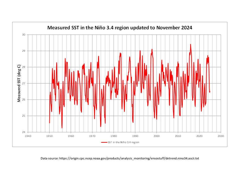
If you look at the measured SST data (not the anomalies), an increasing trend is clear. The maximum monthly measured SST values (El Niño events) and the minimum measured values (La Niña events) both show a long term increase of around 1degC since 1950, while maintaining the min-max range of about 4degC.
You’re conflating actual temperatures with an index.
The ocean temperatures are warming because the oceans are warming, not because the intensity of the ENSO effect has increased.
It’s the reason NOAA has to update its ENSO index every 5 years, as explained here.
Your answer is a trite phrase you have lifted from somewhere.
The ocean temperatures are rising because the oceans are warming! No kidding Sherlock!
The intensity of ENSO has increased. Wow, do you think higher temperature might cause that.
Now, explain the cause of warming Pacific ocean temperatures!
Here is another question. You are prone to dismiss temperature trends in the U.S. because it is a small part of the global area. What is the area of the globe that is covered by ENSO? Why is it such a large part of the global average temperature?
I was not conflating anything. I was explicitly clear that I was referring to actual measured SSTs and not computed anomalies.
I was simply highlighting the fact that this is a classic example of the circular argument. NOAA makes the assumption that the longer term growth in SSTs in the Niño-3.4 region “do[es] not reflect interannual ENSO variability” and it then applies a procedure that removes it as part of the determination of an index.
Along you come and say the ENSO index is absolutely balanced, without mentioning the fact that it was the underlying mathematical process used by NOAA which forced it to be so.
You don’t know what piecewise integration is? You should have learned that in Calc 1.
See here.
https://www.geeksforgeeks.org/definite-integrals-of-piecewise-functions/
The question being posed is “why is there no global warming between El Nino occurrences”?
Your analysis of El Nino’s has no bearing on that.
You don’t know that removing warm periods from a temperature time series will cause it to cool?
You should know that by common sense. No fancy descriptors required.
You don’t know that removing warm periods from a temperature time series will cause it to cool?
Do you see cooling anywhere? All I see is no warming between El Nino’s. Doesn’t that intrigue you at all? CO2 doesn’t disappear between El Nino’s so why does the lack of warming occur. I’ll bet you have no idea how to explain the fact that temperatures do not fall back to pre-El Nino values.
The very trend that is being displayed can not be explained by GHE. Why is that?
What does your common sense tell you about the reason of several years (3 – 7) of no warming, then a sudden, 1 year of warming that remains forever?
It smacks of smoothing a nonstationary time series that results in a spurious trend.
Well El Nino/LaNina is the result of a multiyear oscillation during which heat is pumped into/released from the deep ocean so it shouldn’t be a surprise that there isn’t an increase in the atmospheric temperature when the heat is being pumped into the deep ocean and there is an increase when it is released.
Actually, by definition, warming is a trend and therefore makes the time-series non-stationary with at least the mean varying over time.
If the temperature is percentage of the mean then the variance will also grow over time – an additional reason for it being non-stationary.
If the variance grows then so does the error term in the OLS regression.
Here are some good pages to read
https://www.sciencedirect.com/science/article/pii/S2405918817300405
https://web.ics.purdue.edu/~bvankamm/Files/360%20Notes/09%20-
%20Regression%20with%20Time%20Series%20Data.pdf
I don’t know anyone complaining about a slightly warmer Feb.
Australians?
And your comment is relevant because . . . ?
Maybe you would do better by claiming that you can make air hotter by adding CO2!
Hottest February? What does that even mean? Can you point to somebody who cares?
The Earth’s surface has cooled to its present temperature. Good luck with denying reality.
Well, fairly good laboratory absorption tests can be extrapolated to show that if you double the amount of CO2 in a column of atmospheric air and keep irradiating it with the same amount of sunlight, the sunlight should heat it up a bit….about 4 watts/sq.M. worth at surface…so about a degree at surface….not enough to allow you to change the vegetable mix you grow in your garden…but some years you might get an extra few days of growing season frost free, depending on the local weather….
Yes, the sun heats the atmosphere. Of course, it heats the surface more, so all the atmosphere does by absorbing the Sun’s energy is to keep surface temperatures lower. Tyndall calculated from his observations that about 35% of the insolation doesn’t reach the surface. NASA’s figure is remarkably close.
Your “fairly good laboratory experiment” is just word salad to me. Sorry.
I’m reasonably sure you can’t find any experimental support for the speculation that removing CO2 from air causes a temperature drop. I’m willing to be corrected.
Over to you.
“And your comment is relevant because . . . ?”
This is a post about the February anomaly according to UAH. My comment is about that.
“Hottest February? What does that even mean?”
It means tha average global anomaly as calculated by Spencer et al and published here, for the calender month of February and compared to previous values for February. In this case last year had the highest anomaly and hence was the hottest.
“Can you point to somebody who cares?”
You seem. To care, or else why keep going on about it? Presumably Watts thinks people here care, or else why keep publishing the UAH monthly data? The fact that these bland posts generate so many comments suggest some here fo care greatly about it.
“The Earth’s surface has cooled to its present temperature.”
Thanks for confirming you do care.
It means tha average global anomaly as calculated by Spencer et al and published here, for the calender month of February and compared to previous values for February. In this case last year had the highest anomaly and hence was the hottest.
Quit using the media propaganda that it was “the hottest evah”!
I didn’t say “evah”. I didn’t even say “ever” I’m sure there were some hotter months during the age iof the dinosaurs. Do you really need me to spell out that it was the hottest from the UAH record? Try reading things in context.
It doesn’t hurt to be accurate.
Bellman, I don’t care at all whether Dr Spencer wastes his time. It’s his choice. I’m curious why he bothers, but I can’t be bothered asking.
An “average global anomaly”? A “highest anomaly”? Colour me impressed.Can you send me some in different colours?
I suppose people who believe that adding CO2 to air makes air hotter might care, but I don’t pay much attention to the opinions of people who are obviously detached from reality to that extent.
I assume you wouldn’t be silly enough to claim that removing CO2 from air causes the air to get colder, would you?
Air temperatures on Earth vary from about 60 C to -90 C. How much colder would they get by removing CO2 from the atmosphere? Pretty silly idea, isn’t it?
The satellite record only goes back to 1979.
You need a longer-term view.
It was just as warm in the recent past as it is today, according to the written record.
Considering that every global ‘written record’, 3 of which go back to 1850, set two consecutive new record warmest years in 2023 and 2024 suggests you may be mistaken here.
Hansen (and one of his colleagues) said 1934, was 0.5C warmer than 1998.
The year 2024 high temperature was 0.35C warmer than 1998.
The year 1934, was warmer than the year 2024.
I’m not mistaken.
You’re talking about America, right; not global? And it looks like you’re also trying to narrow it down to summer only; another deceptive slight of hand
Even then, once the many and various biases are properly corrected for, the warmest full years in the US record since 1880 are 2012, 2016, 2017, 2021 and 2023, in that order.
Really? Here are some graphs from various states. They are from NOAA and are all one month values from 1900 through 2024. There are other states that are the same.
Can you guess which states have a large increase? It shouldn’t be real hard to figure them out.
Where do you live? Where I live summertime is when high temperatures occur. It is when maximum insolation is received which will result in maximum “back radiation” from CO2 and will cause maximum temperature rise according to the GHE. In your world does “hottest ever” arrive in winter?
This is a completely cockneyed characterization. Increasing CO2 produces a gradual, long term warming of the climate. It doesn’t have larger seasonal expression in the way you’re suggesting.
You really believe CO2 concentrations aren’t correlated with a seasonal component?
They are explicitly correlated with the northern hemisphere growing season, but not because of CO2 forcing.
So now you are trying to claim that CO2 concentration is not related to CO2 forcing?
The seasonal CO2 cycle is related to primary productivity, and consequently generates no long term forcing of the climate. The long term, gradual rise in atmospheric CO2 concentration is driven by anthropogenic emissions and does produce long term forcing.
Until people start dying from heat waves in the Winter, I don’t think we have much to worry about.
You haven’t answered my questions yet about the lack of warming.
“The satellite record only goes back to 1979.
You need a longer-term view.”
Here’s how the game plays out –
I’ll say, “sure – look at long longer-term data sets. They all show last year was a record”.
Tom will then say – “But I don’t like any of those longer term data sets. They all show it being warmer than in the past – and that’s wrong.”
He’ll then produce the only data set he likes. One produced last century by James Hansen. “This proves temperatures were just as warm in the 1930’s as they are to day, and therefore all other data sets must be wrong. The science is settled.”
I’ll then point out that it’s only for the USA and the global graph produced at the same time shows temperatures warming since the 1930s. Then I’ll point out that by definition a graph produced almost 30 years ago does not show the warming that has happened in the 21st century. If I was being mischievous I might ask why he considers Hansen of all people to be the only reliable source on global temperature analysis.
Tom will then start yelling about “bastardized” data sets. And produce a selection of cherry-picked graphs for individual countries which he will claim all show it being warmer at some point in the past.
I’ll then point out that the graphs he’s using are from BEST, the source he claims is “bastardized”. He won’t see the irony, and the conversation will then go round in circles a few more times.
Unless anyone has anything original to contribute to this – I’ll leave it there for the time being.
Someone apparently wrote –
“The satellite record only goes back to 1979.
You need a longer-term view.”
I can’t think of any longer term view than that from the creation of the surface to now. Extreme cooling as the surface is no longer molten. Any advance?
I have nothing original, but I will concur I have been down this path a few times with good ole Tom. To be fair to him though, he is always respectful in his writings and never (that I have seen) gets personal if you disagree with him.
Thanks, Simon. I appreciate that.
Check out my link just above to 600 historic, regional temperatures charts from around the world, none of which have a “hotter and hotter and hotter” temperature profile.
The “hotter and hotter and hotter” Hockey Stick temperature profile was created using regional temperature data that does not have a “hotter and hotter and hotter” temperature profile, so my question is how do you get “hotter and hotter” out of data that does not have “hotter and hotter”?
I don’t expect you to answer this question. I do expect the Climate Alarmists who portray themselves as experts on charts to answer this question, but to date, it’s “Crickets” from those individuals.
And I know why: Because, for all their bluster, they have no answer. You can’t get blood out of a turnip.
The dataset is a Gish gallop, and it’s impossible to believe it is presented in good faith. Many of the papers are using the same set of proxy records, and those proxy records are included in the datasets used for global paleoclimate reconstructions (e.g. about half of the cited datasets are in the PAGES2k database). The idea that someone can simply eyeball a giant list of disparate and non-overlapping records and determine something about global-scale trends is absurd on its face.
Take all those individual records and compile them into a global reconstruction, and present your results. You haven’t done the actual work yet.
“He’ll then produce the only data set he likes. One produced last century by James Hansen. “This proves temperatures were just as warm in the 1930’s as they are to day, and therefore all other data sets must be wrong. The science is settled.””
I can do better than that. Here are 600 regional, written, historic temperature records from around the world that have a similar temperature profile to the U.S. regional chart (Hansen 1999), which shows it was just as warm in the recent past as it is today.
https://notrickszone.com/600-non-warming-graphs-1/
Do you have 600 regional, historic charts showing a “hotter and hotter and hotter” Hockey Stick temperature profile? Answer: No, you don’t. All you have is one computer-generated Hockey Stick chart. Generated how? is the question. The question that Climate Alarmists can’t answer.
“Here are 600 regional, written, historic temperature records from around the world that have a similar temperature profile to the U.S. regional chart (Hansen 1999)”
I’m not ploughing through 600 reports, but from the ones I’ve seen almost none are talking about it being warmer in the 30s than today. Most are talking a bout the middle ages or further back. Others are only talking about the satellite era.
The only one I saw mentioning the 1930s was about the North Atlantic. And that’s saying just what other data sets show, including the ones you dismiss as “computer generated”.
February is near the middle of the northern hemisphere Winter, typically the month after the coldest month (locally, we see a warming during the month), and near the middle of the seasonal atmospheric CO2 ramp-up phase, albeit February commonly shows decline in the rate of CO2 accumulation. While there is a long-term correlation between CO2 and temperature, short-term they are anti-correlated. I think that you are missing something here.
“While there is a long-term correlation between CO2 and temperature”
Correlation is meaningless unless a functional relationship can be shown. I haven’t worked it out but there is probably a correlation between postal rates and temperature as well.
The pony about short term correlations is that they are going to be very uncertain. Any relationship includes noise, short term variation, and so it’s often possible to see short term negative correlations. That’s why you need to look at the uncertainty. And better look for confounding factors such as El Niños.
Still waiting for the official UAH map, but here’s my own version.
And this is NH Winter 2024/25
And Here’s the absolute temperature map for February 2025.
The world is burning up!
The warmest center shows something around 273K. That’s damn cold for the globe since that’s the area of warmest temperatures in February.
“The world is burning up!”
Is it?
“The warmest center shows something around 273K. That’s damn cold for the globe since that’s the area of warmest temperatures in February.”
How many times does it have to be explained that these are the temperatures of the lower troposphere? Do you really think it’s freezing over the tropics?
Look at the graph. The tropics are in yellow.
That is damn cold.
Here is what you said.
Don’t be a hypocrite. You are the one that suggested this was an accurate portrayal of absolute temperature in relation to a message thread about temperature to CO2 correlation.
If you don’t really believe that this graph is applicable, then don’t try to fool folks with information that is not applicable.
“The tropics are in yellow.
That is damn cold.”
It’s my graph. I’s my colour pallet. I went through lots of possible colour schemes, none if them were entirely satisfactory. You can not tell just by looking at the colour of it’s cold. You need to look at the legend, and even then it’s pretty meaningless as it’s the temperature in the lower troposphere.
“Don’t be a hypocrite”
You keep throwing out insults like this with no understanding of the meaning of the words. Why do you think I’m being hypocritical. I nearly showed what the UAH claims as the average temperature for the lower troposphere. I never claimed I though this is useful. But some here like to claim that anonalies are fraudulent, so thought it interesting to compare the two.
“You are the one that suggested this was an accurate portrayal of absolute temperature in relation to a message thread about temperature to CO2 correlation.”
Again I make no claims about the accuracy of UAH. But this website holds it to be the most accurate as it shows less warming, and is run by the right sort of people.
And this is not a message thread about CO2. It’s about what the data is showing. You might want to conclude that it’s likely that CO2 is a cause of the warming trend, but it isn’t the point of this article.
Here are the ground temperature using BEST. This is for last December, as that’s the most recent data available.
I’ve tried to use a similar palette as the UAH map, but had to shift it up 10K to cover the highest surface temperatures.
The new Monckton Pause extends to 20 months and begins in 2023/06. The average anomaly during this period is 0.71 C.
The previous Monckton Pause peaked at 107 months beginning in 2014/06. The average anomaly during this period was 0.21 C. The trend since the beginning of the pause is +0.37 C.decade-1.
The leap from the previous pause to the current pause is currently 0.5 C.
Thanks for substantiating the fact that El Ninos cause a step change. 🙂
“The leap from the previous pause to the current pause is currently 0.5 C.”
……. thereby adding to the large and growing body of evidence that the warming is not caused by anthropogenic CO2.
Send in the ruler monkeys…
Blind monkeys that cannot, by selective blindness, see the effect of the El Nino events..
Lower troposphere is cooling off. That must be painful viewing for some…
According to RSS, “Microwave sounders are capable of retrieving vertical temperature profiles of the atmosphere by measuring the thermal emission from oxygen molecules at different frequencies.”
So RSS use “thermal emission” (definitely infrared, not visible or ultraviolet) from oxygen, which emits different frequencies dependent on temperature!
Obviously impossible, according to “climate scientists” and their gullible followers, who seem to be convinced that oxygen cannot emit infrared radiation. It seems in practice it can and does, and is used to supply people like Dr Spencer (as far as I know) with data.
So at least one “climate scientist” depends on oxygen emitting infrared radiation, to possibly support a contention that oxygen does not emit infrared radiation!
Regardless, Dr Spencer’s labours are quite pointless. What do they achieve? Nothing at all, that’s what. Air temperature changes, and nobody can predict the future changes better than a 12 year old.
A complete waste of time and effort, but at least he’s getting someone else to pay for it, whether he’s wasting his time is largely irrelevant.
Adding CO2 to air does not make it hotter, and the highest surface temperatures occur where GHGs are least. So much for a GHE.
Many deserts have high temperatures but low specific humidity. I just checked Death Valley. The temperature is 22 deg. C and the RH is 18%.
Harold, exactly. Lack of the most “important” GHG (H2O), results in hotter maximum temperatures. More GHG makes maximum temperature lower.
“Climate scientists” live in a fairytale world, where reality is ignored.
Specific humidity is not relative humidity (RH – https://www.weather.gov/lmk/humidity)
Just a nit….
According to RSS, “Microwave sounders are capable of retrieving vertical temperature profiles of the atmosphere by measuring the thermal emission from oxygen molecules at different frequencies.”
So RSS use “thermal emission” (definitely infrared, not visible or ultraviolet) from oxygen, which emits different frequencies dependent on temperature!
Microwaves are not infrared.
“Microwaves are not infrared.” Of course they are! Infra – below or beneath, red – visible red colour.
“Thermal emission” is just meaningless jargon.
Anyway, hopefully you’re not trying to use semantics to imply that adding CO2 to air makes air hotter.
Just a nit.
You’re the one using semantics rather than science!
The big problem with using microwave emissions is that path loss modulates how much can be received. Water vapor in the path is a major contributor to microwave path loss. Unless UAH can measure the humidity along the path (and I don’t know how they can do that) being measured there is an in-built, systematic measurement uncertainty in their observation. I’ve never seen this quantified anywhere. I do know when I was involved in building microwave links for a telephone company that we had to make allowances for the path loss, including water vapor, when sizing the amount of power needed to insure the operation of the link. So I remain skeptical of the measurement protocol using microwave emission if the measurement uncertainty budget does not include an allowance for path loss.
Similar to link margin analysis.
If the sensor is not measuring amplitude, the losses might be less critical than the frequencies, which as reported, O2 puts out different frequencies based on temperature.
I am still not convinced satellites can accurately, repeat accurately, measure temperatures, definitely not directly like a RTD or thermometer.
“Similar to link margin analysis.”
Exactly what it was called!
It’s my understanding the MSU’s measure the radiance value, not the frequency. The radiance value would depend on the path loss.
Not at the frequencies used in this method. Water emits microwaves in its rotational spectral line at 22.325 GHz whereas Oxygen emits in a rotational band around 60 GHz. I suspect that the microwave band you were using would be the K-band, between 18-27 GHz, so affected by H2O but not O2.
That’s why I soke of water vapor. But there are other things as well such as dust that can cause scattering and affect path loss. It all contributes to the measurement uncertainty of UAH data. But I never see path loss mentioned in association with UAH.
That’s why they don’t use Channel 1.
“MSU Channel 1 is not used to monitor atmospheric temperature because it’s too much sensitive to the emission from the surface, furthermore it is heavily contaminated by water vapor/liquid water in the lowermost troposphere.”
There are ways to estimate water vapor but like all “estimates” they are accompanied by an uncertainty factor. It’s like the parameterization of cloud cover in the climate models. The problem is not the estimating itself, it’s refusing to admit to the uncertainty it causes.
Once again you reveal your complete lack of knowledge of Physical Chemistry, in this case the interaction of radiation with molecules!
“According to RSS, “Microwave sounders are capable of retrieving vertical temperature profiles of the atmosphere by measuring the thermal emission from oxygen molecules at different frequencies.”
So RSS use “thermal emission” (definitely infrared, not visible or ultraviolet) from oxygen, which emits different frequencies dependent on temperature!”
Microwave, not infrared!
“Obviously impossible, according to “climate scientists” and their gullible followers, who seem to be convinced that oxygen cannot emit infrared radiation. It seems in practice it can and does, and is used to supply people like Dr Spencer (as far as I know) with data.”
No according to physical chemists, as you would have found out had you taken a freshman course on the subject.
To absorb infrared radiation a molecule must have a dipole (e.g. H2O and CO2), N2 and O2 don’t possess a dipole and so don’t absorb/emit IR (vibrational excitation). The IR frequencies involved are of the order of 10µm. The microwave wavelengths used are of the order of 0.5cm and are the result of the interaction of the magnetic moment of the O2 molecule with electromagnetic fields (rotational excitation). O2 is paramagnetic due to the presence of unpaired electrons.
“So at least one “climate scientist” depends on oxygen emitting infrared radiation, to possibly support a contention that oxygen does not emit infrared radiation!”
No he understands the well established science of Physical Chemistry and molecular structure and the difference between IR and microwave radiation (in this case a factor of 500 in wavelength)!
Smith, K.E., et al. 2025. Ocean extremes as a stress test for marine ecosystems and society. Nature Climate Change. https://doi.org/10.1038/s41558-025-02269-2
“In 2023–2024, widespread marine heatwaves associated with record ocean temperatures impacted ocean processes, marine species, ecosystems and coastal communities, with economic consequences. Despite warnings, interventions were limited. Proactive strategies are needed for inevitable future events……Marine Heatwaves International Working Group (https://www.marineheatwaves.org)” Acknowledged support almost as long as the 15 references all in the new millennium that they worry about. There are not enough historical ocean measurements to know about a “record heat wave” and all their claimed effects.
Two of the 13 authors locations— “Institute for Marine and Antarctic Studies and ARC Centre of Excellence for Climate Extremes, University of Tasmania, Hobart, Tasmania, Australia.” Ocean gets hot in Tasmania without lava flows? Somebody actually pays $29.99 for this paper?
From the marine heatwave site –
“Most marine heatwaves in the Arctic are generated by taking atmospheric heat up and disappear when this heat is transferred to the deeper ocean.”
Nonsense. For several reasons – if the ocean surface as warmer than the atmosphere, no atmospheric heat will be absorbed
If the blazing arctic sun manages to warm the surface with its furious radiance, the warmer water will just sit on top of the colder, denser water already there.
Transferring surface heat to deeper water is just silly, as any heat radiated to adjacent lower water will result in warmer, less dense water, which will promptly rise to the surface.
All about as stupid as claiming that surface winds create deep ocean currents – they don’t. The ocean is heated from below, and deep ocean currents are due to convection. Hotspots occur in the ocean basin crust, and move around erratically, resulting in warmer water above them. These hotspots are visible to satellites measuring sea surface temperatures.
No GHE needed.
There is no such thing as a ”marine heatwave”.
Also, are you saying that a billion years of sunshine beating down on the equatorial ocean has had no effect on deep ocean temps? I find that highly questionable.
“Also, are you saying that a billion years of sunshine beating down on the equatorial ocean has had no effect on deep ocean temps? “
Yes indeed. Warm water floats. If you have any questions, I can probably answer them for you.
It is why ponds overturn. As winter starts, the surface water cools and sinks while the warmer water at depth rises.
Jim, indeed. And that is why oceans and deep lakes don’t freeze right through.
Because freshwater has a maximum density at 4ºC, so when the surface reaches that temperature the water overturns until it all reaches that temperature and then the surface can start to freeze. In the spring as the surface warms up to 4ºC the density increases and overturning occurs again. Sea water has no such maximum, in the arctic the overturning is the result of high salt content water from new ice sinking as a result of its higher density, see Halocline.
Yes I am aware that warm water floats but you are suggesting that an atmosphere warmer than the ocean would have no effect of that body of water. That is untrue. If you have ever waded in the shallows at a beach on a hot day you will notice the water has been warmed from above. That does not preclude warming from the bottom up as well.
You say “you are suggesting that an atmosphere warmer than the ocean would have no effect of that body of water.” I’m not suggesting any such thing, and you haven’t quoted me saying anything to that effect.
Of course warmer objects transfer their energy to colder ones.
Yes, the water is warmed by the Sun. In a properly constructed solar pond, temperatures of over 90 C can be obtained, but solar ponds prove to be fairly useless as a source of even hot water for many practical reasons.
Beach shallows and tidal pools get pretty hot. Even more exciting is jumping into a lake where the top few centimeters are hot, and then experiencing frigid water below.
Warming the top layer until it boils into steam is pretty easy. The water beneath stubbornly refusing to heat if its base remains cool. At about 10 km depth, water temperature may be 1C. The temperature of the ground at 10 km is around 250 C to 300 C.
So you have a large hot bucket full of very cold, just above freezing, water, with a surface temperature maybe 30 C. Basic physics. Convection ensues.
Adding CO2 to air doesn’t make it hotter, though, does it? Basic physics.
That is the case because cold, dense polar waters sink and travel below the thermocline. The sun only warms the upper couple of hundred meters even in the tropics, and less in the polar regions because sunlight enters the water obliquely (high angle of incidence) near the poles.
High evaporation rates in the tropics removes water and encourages upwelling, which helps drive the currents.
Clyde, all water cools and sinks. Water cooling at the North Pole sinks just like water at the Equator. And then what does it do? Travel around a globe with the center of gravity in the middle?
No – all around the globe cold water sinks towards the center of the globe! And would remain in situ forever, except for convection caused by being heated from beneath – and from the sides of the basins of course. That’s why all bottom water is the temperature at which it is densest.
People might be looking at a globe on a desk imagining cold water from the North Pole running over the surface towards the Equator, for all I know. The same people might believe that adding CO2 (or H2O) to air makes it hotter.
Ok, we are in agreement. I must have misunderstood when Michael Flynn said ” The ocean is heated from below ”
Thermal conductance by depth does happen in the ocean. There will be a thermal gradient and it is not so simple as you phrased it.
That said, two primary sources of thermal energy are present a the surface: the atmosphere and the sun.
You are correct on this point: if the atmosphere is cooler than the ocean surface, no thermal energy flows from the air into the water. In fact, it flows the other direction.
Your simplified explanation of ocean currents is incomplete.
“Your simplified explanation of ocean currents is incomplete.”
Well, your “Thermal conductance by depth does happen in the ocean” is incorrect – physically impossible for the reasons I describe.
But hey, who knows, I may be wrong.
Could you be helpful, and complete my incompleteness to assist others? You won’t mind if I ask you to back any assertions with reproducible experimental evidence, will you?
For a start you don’t consider the effect of salinity.
And the warm, mixed layer is separated from the cold abyssal water by the thermocline.
Does anyone know why the website https://temperature.global/ is now not available?
SPAM. I bit, so you all don’t have to.
Thanks. I owe you one.
Here is a monthly comment about the UAH anomalies and Australia in the lower troposphere.
This month, my graph (with thanks to Dr Spencer and the team) is shown post year 2015. This gives a reasonable view of the shape of the large (both high and wide) peak that is persisting since its start about March 2023.

Both the width and the month-to-month texture are unusual compared to previous peaks over Australia.
Because of the frequent mention of the eruption at Tonga in Dec 2021, I have colored the period from eruption to now in orange. It is hard to conclude that Hunga Tonga influence is present, but it is also hard to conclude that it is absent.
Here is the graph. Geoff S