From Dr. Roy Spencer’s Global Warming Blog
by Roy W. Spencer, Ph. D.
2024 Sets New Record for Warmest Year In Satellite Era (Since 1979)
The Version 6.1 global average lower tropospheric temperature (LT) anomaly for December, 2024 was +0.62 deg. C departure from the 1991-2020 mean, down slightly from the November, 2024 anomaly of +0.64 deg.

The Version 6.1 global area-averaged temperature trend (January 1979 through December 2024) remains at +0.15 deg/ C/decade (+0.22 C/decade over land, +0.13 C/decade over oceans).
As seen in the following ranking of the years from warmest to coolest, 2024 was by far the warmest in the 46-year satellite record averaging 0.77 deg. C above the 30-year mean, while the 2nd warmest year (2023) was +0.43 deg. C above the 30-year mean. [Note: These yearly average anomalies weight the individual monthly anomalies by the number of days in each month.]

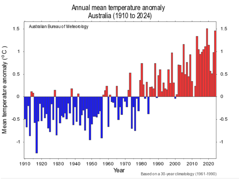
The following table lists various regional Version 6.1 LT departures from the 30-year (1991-2020) average for the last 24 months (record highs are in red).
| YEAR | MO | GLOBE | NHEM. | SHEM. | TROPIC | USA48 | ARCTIC | AUST |
| 2023 | Jan | -0.06 | +0.07 | -0.19 | -0.41 | +0.14 | -0.10 | -0.45 |
| 2023 | Feb | +0.07 | +0.13 | +0.01 | -0.13 | +0.64 | -0.26 | +0.11 |
| 2023 | Mar | +0.18 | +0.22 | +0.14 | -0.17 | -1.36 | +0.15 | +0.58 |
| 2023 | Apr | +0.12 | +0.04 | +0.20 | -0.09 | -0.40 | +0.47 | +0.41 |
| 2023 | May | +0.28 | +0.16 | +0.41 | +0.32 | +0.37 | +0.52 | +0.10 |
| 2023 | June | +0.30 | +0.33 | +0.28 | +0.51 | -0.55 | +0.29 | +0.20 |
| 2023 | July | +0.56 | +0.59 | +0.54 | +0.83 | +0.28 | +0.79 | +1.42 |
| 2023 | Aug | +0.61 | +0.77 | +0.45 | +0.78 | +0.71 | +1.49 | +1.30 |
| 2023 | Sep | +0.80 | +0.84 | +0.76 | +0.82 | +0.25 | +1.11 | +1.17 |
| 2023 | Oct | +0.79 | +0.85 | +0.72 | +0.85 | +0.83 | +0.81 | +0.57 |
| 2023 | Nov | +0.77 | +0.87 | +0.67 | +0.87 | +0.50 | +1.08 | +0.29 |
| 2023 | Dec | +0.75 | +0.92 | +0.57 | +1.01 | +1.22 | +0.31 | +0.70 |
| 2024 | Jan | +0.80 | +1.02 | +0.58 | +1.20 | -0.19 | +0.40 | +1.12 |
| 2024 | Feb | +0.88 | +0.95 | +0.81 | +1.17 | +1.31 | +0.86 | +1.16 |
| 2024 | Mar | +0.88 | +0.96 | +0.80 | +1.26 | +0.22 | +1.05 | +1.34 |
| 2024 | Apr | +0.94 | +1.12 | +0.77 | +1.15 | +0.86 | +0.88 | +0.54 |
| 2024 | May | +0.78 | +0.77 | +0.78 | +1.20 | +0.05 | +0.22 | +0.53 |
| 2024 | June | +0.69 | +0.78 | +0.60 | +0.85 | +1.37 | +0.64 | +0.91 |
| 2024 | July | +0.74 | +0.86 | +0.62 | +0.97 | +0.44 | +0.56 | -0.06 |
| 2024 | Aug | +0.76 | +0.82 | +0.70 | +0.75 | +0.41 | +0.88 | +1.75 |
| 2024 | Sep | +0.81 | +1.04 | +0.58 | +0.82 | +1.32 | +1.48 | +0.98 |
| 2024 | Oct | +0.75 | +0.89 | +0.61 | +0.64 | +1.90 | +0.81 | +1.09 |
| 2024 | Nov | +0.64 | +0.88 | +0.41 | +0.53 | +1.12 | +0.79 | +1.00 |
| 2024 | Dec | +0.62 | +0.76 | +0.48 | +0.53 | +1.42 | +1.12 | +1.54 |
The full UAH Global Temperature Report, along with the LT global gridpoint anomaly image for December, 2024, and a more detailed analysis by John Christy, should be available within the next several days here.
The monthly anomalies for various regions for the four deep layers we monitor from satellites will be available in the next several days at the following locations:
The chart of ranked annual averages is astonishing – 2024 was a huge departure even against the long term warming trend. There’s nothing like it in the historic record.
Hunker down and pray Al.
There’s nothing else humanity can do to exist.
(Except maybe dial the air conditioners to 21 instead of 22).
How old is earth?
According to AlanJ, the Earth was formed in 1979!
Funny how you put words in AlanJ’s mouth that he did not say. He simply observed what we can all see, that 2024 is a dramatic departure (anomaly?) in the satellite record. It doesn’t mean CO2 or humans were the cause. In fact the sudden increase essentially refutes the notion that CO2 or humans were the cause, since neither changed dramatically in 2024. The sudden—and likely transient—warming is just an interesting fact. I’m curious to know what the primary drivers are. Some have suggested the Hunga Tonga volcano ejecting a massive plume of water vapor into the upper atmosphere. Maybe. Whatever the reason, it would be interesting to know.
Alan J said, “There’s nothing like it in the historic record.”
We don’t have records for the whole of the earth before around 1900 and even then measurements were sparse. However, we do have proxy records that indicate global temperatures were higher than today many times in unrecorded history.
Alan has put the words into his own mouth.
“ However, we do have proxy records that indicate global temperatures were higher than today many times in unrecorded history.”
Gotta link to those proxy records soldier? I know the earth has been hotter in the past, but been keen to see when your proxy records say that is?
Nearly all the last 10,000 years have been warmer than now.
Tree line, permafrost, trees under glaciers, animal remains in the far north etc etc
Seems you are a “climate denier.”
“Nearly all the last 10,000 years have been warmer than now.”
How can I put this? Bullshit. Not even close….
https://news.arizona.edu/news/global-temperatures-over-last-24000-years-show-todays-warming-unprecedented
https://science.nasa.gov/climate-change/evidence/
Your turn “Mr Nonsense?”
Funny how when you ask Mr Nice2000 for specific information to back up his nonsense, he runs for the hills. He’s good like that.
Care to explain why the fields where the Greenland Vikings once grew barley and rye are under permafrost today?
Ten seconds using the WUWT search function gives this as first result:
From Russia to the Indian Ocean to Antarctica, surface temperatures were much warmer than they are today during Medieval times.
1. The Eastern Russia region was 1.5°C warmer than now during the Medieval Warm Period. The modern warm-up began centuries ago and temperatures have declined in the last few centuries. Relative sea levels were 1 m higher than now 1,000 years ago.
“From Russia to the Indian Ocean to Antarctica, surface temperatures were much warmer than they are today during Medieval times.”
Yes I have an excellent explanation. It’s not true. It’s a myth that is pumped here regularly. It just has no basis of truth. It’s a stretch at every level to believe this. Sure some parts were warm, but it is simply false to say the warming was global.
But… even if what you say is true (and it’s not) what Benice2000 said was “Nearly all the last 10,000 years have been warmer than now.”
And that is provably, beyond doubt, 100%, bet your mother on it……false.
Feel free to rebut the dozens of papers which show that the Holocene, Minoan, Roman, and Medieval Warm Periods were global in extent and warmer than today.
Don’t need to. Been through this numerous times.
No you haven’t.
What? That’s a bit arrogant. Yep I have. The offical peer reviewed line is the Medieval Warm period is a real thing, but unlikely to be:
a) as warm as today
b) global
But here’s the thing. If it was as warm as today, or let’s say warmer, then something forced that warming. And if the climate can react that quickly then that is cause for concern. Many argue the MWP gives us greater cause for concern with the increase in CO2, not less.
All the papers I have cited are wrong? Please post the rebuttals then.
What is this “official peer-reviewed line”?
Be careful of the NASA link – while it claims that “the current warming is happening at a rate not seen in the past 10,000 years”, the graph it presents is a scary one showing CO2, not temperature.
The Arizona study chooses a strange time period of 24,000 years, which shows the transition from full glacial to the current interglacial. There were 4 previous Milankovitch-driven glacial/interglacial cycles where interglacial temperatures appear higher than today.
The best outcome for planet earth would be for the current interglacial warming to over-ride a cyclic transition into another ice age.
“The best outcome for planet earth would be for the current interglacial warming to over-ride a cyclic transition into another ice age.”
I would argue the best outcome for humans on earth would be to live in a climate that is stable.
When has climate ever been stable? What makes you think Man can influence it?
By stable I mean as it has been for the last 20 odd thousand years. A few ups a few downs. And I also mean not changing quickly as it is now.
The climate is changing faster today than it did during the Dryas and Younger Dryas?
The climate is changing faster today than at any time in the last 100k years. That’s significant because that is when human beings have evolved and flourished. If we want to keep flourishing and supporting the billions who now live and and are sustained by this planet, then common sense would tell us a stable climate is in our best interest.
How do you know current CC is more rapid than during the Dryas?
Take a look at the graph I posted above that will tell you.
And read the peer review paper I posted that will tell you.
And read the Nasa reference I posted that will tell you.
I can get more if you want, but I’m sure you get the idea.
From the IPCC itself:
The central Greenland ice core record (GRIP and GISP2) has a near annual resolution across the entire glacial to Holocene transition, and reveals episodes of very rapid change. The return to the cold conditions of the Younger Dryas from the incipient inter-glacial warming 13,000 years ago took place within a few decades or less (Alley et al., 1993). The warming phase, that took place about 11,500 years ago, at the end of the Younger Dryas was also very abrupt and central Greenland temperatures increased by 7°C or more in a few decades (Johnsen et al., 1992; Grootes et al., 1993; Severinghaus et al., 1998
Now push right off, you little liar.
What a sad man.
When you can come up with a “global” reference in a peer reviewed paper (as I have) that says the dryas was warmer than today, then you have some reason to abuse me. Till then you are just another light weight rearranging the deck chairs, trying to fool with bullshit and bluster.
The climate is changing faster today than at any time in the last 100k years.
Your words, not mine.
Where did I assert that the Dryas or Younger Dryas were warmer than today? I said that you were lying when you said the rate of CC is the fastest in 100 K years.
Plenty of peer-reviewed references in the extract from the IPCC report.
Slimy troll.
“Plenty of peer-reviewed references in the extract from the IPCC report.”
Yup but not global. End of story. Yawn…..
Where did I claim the Dryas and Younger Dryas were global? The Northern Hemisphere is a pretty big place, BTW.
You were the one who claimed the rate of current CC is unprecedented. You were lying, ass usual.
“You were the one who claimed the rate of current CC is unprecedented. You were lying, ass usual.”
Yup globally it is, and that’s what counts. If you are childishly trying to claim that a part of the planet was warmer at one time than another part of the planet … then wop-de-do. What a clever man you are…… You got me there. Except Einstein, I never claimed that.
Plenty of places cooler than during the 1930’s (Australia, US).
Lies upon lies from the little troll Simon.
Yes but not globally. Are you deliberately being silly? If not you a bloody good at it.
Look at my post just above this one. I show stations from all over the globe with no or little CAGW temperature increase. Most have records that are over 100 years long. There are lots more.
Why don’t you tell everyone how this could happen? You obviously know how this isn’t happening.
No post by you above this one…..
No post by you above this one…..
Ok try again.
Here are six locations from around the globe. Greenland, Peru, Japan, Europe, and the U.S. It certainly isn’t comprehensive, but it does indicate that warming shouldn’t be classified as “global” because it is not occurring EVERYWHERE.
Lot’s of cherry-picking there. Different time periods, different styles of graphs, but also little evidence that they haven’t all warmed.
I’ve already shown that Montana has a warming trend since 1900.
Is your Japanese winter graph taking into account changes in stations? That’s the usual trick used by the author of those Japanese graphs.
Here’s the UAH global winter data over that period.
Japan has actually been warming during Winter according to UAH. If you wanted to cherry-pick a region you would be better using northern locations, such as Northern Europe.
“Plenty of places cooler than during the 1930’s (Australia, US).”
Untrue
Here are some local graphs from stations all over the globe. Why do you think this many don’t have CAGW from the CO2 concentration increase?
“Here are some local graphs from stations all over the globe. Why do you think this many don’t have CAGW from the CO2 concentration increase?”
Let me ask you a question. Do you genuinely think that by popping up a few random graphs from a tiny fraction of the globe that you somehow override the overwhelming consensus that we have had global warming?
And yes it is entirely understandable that even as CO2 rises there will be pockets of the globe cool. That is climate change 101.
Global warming! You use that term and can’t even admit that not everywhere has warmed.
I’ve shown you “random” sites from all over the globe! That provides a counterexample to your assertion. In logic AND science that is sufficient to declare the assertion false.
You need to provide an exception and rule that allows for sites that have no warming. Good luck.
From:
https://quillbot.com/blog/reasoning/ad-populum-fallacy/
As bnice continually asks, where is the evidence that supports the assertion?
“Global warming! You use that term and can’t even admit that not everywhere has warmed.”
Yes… Yes I can. That’s how it works.
“I’ve shown you “random” sites from all over the globe! That provides a counterexample to your assertion.”
Yes you have and they prove literally nothing except you know how to find random graphs from all over the globe. Congratulations.
“You need to provide an exception and rule that allows for sites that have no warming. Good luck.”
No I don’t. And do you know why? Because anyone who knows anything about this subject knows the planet does not heat and cool uniformly. It’s why they came up with the term “microclimate.” What is important is whether or not the average temperature of the planet is going up or down, and right now it is mot definitely going up and is now at temperatures not seem for 100k years. Here is my evidence….
https://news.arizona.edu/news/global-temperatures-over-last-24000-years-show-todays-warming-unprecedented
https://science.nasa.gov/climate-change/evidence/
I’ll look forward to yours….
“As bnice continually asks, where is the evidence that supports the assertion?”
OK you are now scraping the bottom of the barrel. Bnice is a silly old fool (being kind here) who wants to remain a silly old fool. There is nothing would convince him that CO2 is warming the planet. Nothing. He has been given countless amounts of evidence and all he does is stomp his feet like a three year old and say you can’t make me agree.
Now the challenge I give to you is to quote a scientist working in the field who says CO2 is not warming us. You wont find one. Not Roy Spencer. Not Judith Curry. They all accept the science they just don’t think the outcome is worth the effort to change what we do.
Meanwhile almost all nationally representative scientific bodies on the planets accepts the human caused increase in CO2 is causing us to warm and that that warming may well result in problems going forward. Here is the Royal Societies (one of the most respected groups anywhere) explanation that clearly tells it how it is.
https://royalsociety.org/news-resources/projects/climate-change-evidence-causes/basics-of-climate-change/
Enjoy….
https://cognitive-liberty.online/argumentum-ad-lapidem-appeal-to-the-stone/
As before, if this is what you have degenerated to, you have lost the argument.
Don’t expect any comprehensive responses since you’ve already indicated that you have no ability to present a cogent argument with supportive evidence.
All I am going to respond with is an Argumentative Fallacy.
That my friend is the response of a man who has no response.
And you sent me to a crazy right wing propaganda site. Why would you think in any way that is proof of anything to do with climate? I read a few of the headlines and OMG that is down the rabbit hole conspiracy stuff. If you are sending me there, I’m afraid you are on the wrong side of the sane debate re science.
Are you looking in the mirror? I gave you a web site and not a simple assertion of my own making.
I sent a link to a resource. That is something you never do, just hand wave as you dance around the tree.
Good luck in ever winning an argument by using fallacies.
There is some messed up content on that website. Topics range from the promotion of brainwashing to the rejection of the link between HIV and AIDS and everything in between.
Do you realize you just used an Argumentative Fallacy?
You need to address the link I gave and refute what it says, not what info is on other pages. Look up red herring.
He’s pointing out that the website has about as much credibility as a Trump wedding ring. And he is right. If you are referencing that as some harbour for truth….. you just lost us.
ROTFLMAO! You are unable to refute the information on the link I gave, so you declare a red herring that other information on the web site you don’t like, therefore that makes everything wrong on this page.
You are a loser when it comes to making cogent and logical argument.
Here is what the website I linked said.
Here is what Wikipedia says. It confirms the web page I referenced. Too bad. Why don’t you post a reference the refutes the info on both pages?
https://wattsupwiththat.com/2025/01/03/uah-v6-1-global-temperature-update-for-december-2024-0-62-deg-c/#comment-4021739
I wouldn’t call Wikipedia a right wing site by any means. Why didn’t you do some research before making another logical fallacy?There is a ton of info on the Internet about the fallacy of appeal to the stone.
I’ll bet you never had a symbolic logic class from the Philosophy Dept. have you. It teaches you how to logically think about solving a set of circumstances to reach a decision.
“I’ll bet you never had a symbolic logic class from the Philosophy Dept. have you……”
Ok…. We might just leave it there. This all makes sense now.
Don’t assume anything. My degree is BSEE and I graduated with 174 hours. Lot’s of different subjects.
The other name for this argumentative fallacy is Argument by Dismissal – an argument is rejected with no actual refutation provided. Typically accompanied by an ad hominem against the source as justification for the dismissal.
“Malarky.”
You’ve just described most comments here, especially from the likes of karlomonte.
You really need to check the fallacy of argument by fallacy. Saying “universities do not define reality” is not intended to be an argument. It’s a statement of my opinion you can disagree with if you want. It is my refutation against the claim that if a university says something is true it must be true.
This is an assertion, proposition, opinion, whatever you want to call it. It may even be true in most liberal arts classes. It is not true in the physical sciences taught in universities. It is why theories must be presented with a mathematical relationship that can predict outcomes. It is the math that defines reality and the university teach the math, therefore, universities DO define reality by teaching the math.
“It may even be true in most liberal arts classes.”
I’d say it’s true for any institution.
“It is not true in the physical sciences taught in universities.”
Really? You think physical science universities “define reality”? Are you going to present an argument, or are you just kicking that stone?
“It is the math that defines reality…”
math != university laboratory. And it’s still debatable.
My question remains, what is the mathematical proof used to claim that the resolution of a mean cannot be higher than that of the individual measurements?
The resolution uncertainty is resolution / sqrt (12).
See section H.6 of the GUM. Specifically Equation H.38 in Section H.6.4.
Notice in example H.6 that the resolution uncertainty (included in the u(d) budget in equation H.35) is propagated assuming r = 0 as shown in equation H.38 which is based on H.34. H.34 itself is equation 16 with r = 0 for all variables using the measurement model in H.33a.
For the sake of furthering the discussion consider what happens when H.33a is divided by 4. H.34 and by extension 4.38 also would have a division by 4 on the rhs per the application of equation 16 (or 10). That means the resolution uncertainty component gets scaled by 1/4.
The salient point is that when the measurement model has a divide by N then the square of the resolution uncertainty component (and other components as well) get divided by N as well when r = 0.
H.6, para. 2:
Completely irrelevant to averaging air temperatures across the globe, the indentations do not vary with time! You seem to have overlooked the important phrase right at the start of H.6.3.1: “Uncertainty of repeated observations.”
H.35 is the RSS of the repeated measurements and the Type B uncertainty of the resolution, as oc pointed out.
This is nonsense, you are ignoring this only applies to repeated observations! (as usual).
That probably doesn’t matter all that much where resolution is concerned. Each measurement is subject to resolution uncertainty whether it involves repeated measurements of a single measurand or single measurements of multiple measurands.
great news
You may have misread that. It’s the u(d_bar) budget rather than u(d)
Well, of course the terms have r = 0.
The standard uncertainty equation is already for an average. Note that the first term is s^2 (d_k) / 5, which is the square of the SEM of depth measurements.
Why ever would somebody do that?
Apart from anything else, it implies the measurements were taken to 4x the resolution.
Are you going for a larger sample size, 4 samples, or a different hardness?
Or are you dividing by 4 because you’ve made a bulk measurement similar to the ream of paper example?
Yes, that is the intention of bulk measurements. I think Taylor has an example with 200 sheets of paper.
Yes of course. Typo. Another typo in my post is that “4.38” should have been “H.38”.
Sorry. I was typing on my phone and had hoped my intent would be more obvious than it was. It’s a hypothetical scenario that transcends H.6. The measurement model in H.6 is in the general form y = a+b+c+d. What if instead we change that to a scenario in which it is y = (a+b+c+d)/4 such that the measurement model includes a division by 4 now. Assume u(a) includes that δ resolution uncertainty and that r = 0 for all combinations of a, b, c, and d not unlike what the GUM assumed in H.6. The variables can represent anything you want. What happens to u(y)^2 and u(y) then? What happens to u(y)^2 and u(y) if we further generalize the measurement model to one with N variables and a division by N?
That would be a bulk measurement, such as Taylor’s example of measuring a stack of 200 sheets of paper or my earlier example of a ream of paper.
The resolution uncertainty term of the stack is the same whether it’s a single measurement or the average of multiple measurements, as per H.34.
Yes, each individual item in the stack is assigned 1/N of the resolution uncertainty.
The critical factor is that the single resolution uncertainty applies to the stack. Measuring each item in the stack individually introduces a resolution uncertainty for each.
What you overlook is that to do so requires N to be treated as a variable, it is not a constant. I solved this problem already below using Eq. 12.
[ u_c(y) / y ]^2 = sum[ p_i * u_i(x_i) / x_i ]^2 or
u_cr(y)^2 = sum[ p_i * u_r(x_i) ]^2
X_bar = sum(X_i) / N
u_cr(X_bar)^2 = (1)^2 * u_r[ sum (X_i) ]^2 + (-1)^2 * u_r(N)^2
u_cr(X_bar)^2 = u_r[ sum (X_i) ]^2 + u_r(N)^2
If the uncertainty of N is small or zero, then
u_cr(X_bar)^2 = u_r[ sum (X_i) ]^2
No root(N).
Do you really not see that saying the relative uncertainty of the mean equals the relative uncertainty of the sum, implies that the absolute uncertainty of the mean is equal to the absolute uncertainty of the sum divided by N?
relative uncertainty = u(quantity) / quantity
convert them back to absolute:
u_cr(X_bar) * X_bar = u_r[ sum (X_i) ] * sum (X_i)
u_c(X_bar) = u[ sum (X_i) ]
still no root N
“u_cr(X_bar) * X_bar = u_r[ sum (X_i) ] * sum (X_i)
u_c(X_bar) = u[ sum (X_i) ]”
Wrong.
“u_cr(X_bar) * X_bar = u_r[ sum (X_i) ] * sum (X_i)”
Is wrong. You’ve multiplied both sides by different amounts. X_bar on the left, sum (X_i) on the right.
Multiply both sides by the same value X_bar, and remember that X_bar = sum (X_i) / N.
u_cr(X_bar) * X_bar = u_r[ sum (X_i) ] * X_bar
=> u_cr(X_bar) * X_bar = u_r[ sum (X_i) ] * sum (X_i) / N
=> u_c(X_bar) = u[ sum (X_i) ] / N
But we could trade equations all day. If you can’t see that 1% of 20 is smaller than 1% of 2000, I doubt you are going to be persuaded by algebra.
No root(N) in here.
If the relative uncertainty of the sum is 1%, the relative uncertainty of the mean is also 1%.
This is what Eq. 12 is telling (the same result can be obtained with Eq. 10).
“No root(N) in here.”
No. It’s N, not root(N). As I’ve said from the start, if the uncertainty of the sum of 100 thermometers is ±5°C, the uncertainty of the average is 5 / 100 = 0.05°C.
“If the relative uncertainty of the sum is 1%, the relative uncertainty of the mean is also 1%.”
Good, so we are all agreed that the relative uncertainty of the average is the same as the relative uncertainty of the sum. Now what do you think that does to the absolute uncertainty of an average. Does it get larger as N increases or does it get smaller?
And do you not see that the average uncertainty is a meaningless number.
Look at it from a measurement standpoint not some math possibility.
A measurement of the same thing has a probability distribution made up of the observations you take of that given measurand . I take 10 measurements of that measurand and find it reasonable to assume it is Gaussian. I find the mean by adding the observations and divide by 10. Then find the variance as usual. If the observations are Gaussian and random, I determine the standard deviation of the mean for the uncertainty. I have now completed the determination of “a”. Then I proceed to do the same for “b, c, d”. The combined uncertainty is determined by the correct addition of the uncertainties of each input variable, not an average of all four uncertainties.
You and bdgwx are wanting to skip the process of analyzing the probability distribution of a series of measurements which results in the average and variance.
If you would read any of the metrology info and really analyze it you would know that defining a function is defining the INPUT QUANTITIES. Therefore, you get what the GUM 4.2 says.
y = f(a, b, c, d).
That is, “a, b, c, d” are unique and independent measurands that are called input quantities. Each “a, b, c, d” has its own unique and independent uncertainty which are added to find a combined uncertainty.
As old cocky has pointed out, what you are trying to do is scale everything by a value, in your case by “n”. However, “n” can be any value, not just the number of terms you “average”. I will agree that if I take an auto and scale the measurements by 1/24th, I will probably also scale the uncertainties.
“And do you not see that the average uncertainty is a meaningless number.”
The uncertainty of the average. Not the average uncertainty. And, no, I don’t think it’s a meaningless number, given that it’s what we’ve been arguing about for the last 4 years. If you think it’s meaningless, why do you worry about how large it is?
“Look at it from a measurement standpoint not some math possibility.”
Measurement is math.
“A measurement of the same thing has a probability distribution made up of the observations you take of that given measurand.”
You keep saying that, and I’m not sure if it’s even worth correcting you at this point. The observations do not make up a probability distribution. They are random values taken from a probability distribution.
So anyway, you describe finding the experimental standard deviation of the mean of four different values. And say
“The combined uncertainty is determined by the correct addition of the uncertainties of each input variable, not an average of all four uncertainties.”
And the correct propagation, assuming you are taking an average of the four values is given by using the law of propagation, with the function (a + b + c + d) / N. Which is karlo correctly points out leads you to the uncertainty of the sum of the 4 values divided by 4,
Uc(Avg) = Uc(Sum) / 4
or dividing through by the average gives
Uc(Avg) / Avg = Uc(Sum) / Sum
“You and bdgwx are wanting to skip the process of analyzing the probability distribution of a series of measurements which results in the average and variance.”
It doesn’t matter what the process is. You can use your 4 mean values, as a Type A uncertainty, or you can use a Type B uncertainty. The point we are trying to make is regardless of how you came by the uncertainties, you need to understand how to use the law of propagation. Everything you keep saying is just trying to distract from the obvious point, that the law does not result in uncertainties increasing the more things you average.
“Therefore, you get what the GUM 4.2 says.y = f(a, b, c, d).”
Yes, that’s what a function looks like. I’ve no idea why you keep pointing out these things as if they were some sort of magic.
“Each “a, b, c, d” has its own unique and independent uncertainty which are added to find a combined uncertainty.”
They might have different uncertainties, we are assuming they are independent, that’s a basic assumption of equation 10. But you are not just “adding” the uncertainties. You are multiplying each by the partial derivative and adding in quadrature.
“what you are trying to do is scale everything by a value, in your case by “n”.”
Yes, that’s what happens. If you would try to understand why the equation works, you might realize that scaling any value is the most basic application of the general law. If the function is Cx, where C is a constant, then the derivative is C, and the uncertainty is multiplied by C. If that wasn’t true then none of it would work.
“However, “n” can be any value, not just the number of terms you “average”.”
Yes, that’s the point. But in the case of an average 1/n is the scaling factor.
“You keep saying that, and I’m not sure if it’s even worth correcting you at this point. The observations do not make up a probability distribution. They are random values taken from a probability distribution.”
If they don’t make up a distribution then how do you get any statistical descriptors? Statistical descriptors describe the distribution of a set of values.
The GAT is a statistical descriptor of a set of observations. If that set of observations doesn’t make up a distribution then the GAT is meaningless – which is what many of us have said for years.
“If they don’t make up a distribution then how do you get any statistical descriptors?”
The statistical descriptors are for the sample. They are estimates of probability distribution the sample came from.
Yes, that is the intention of bulk measurements. I think Taylor has an example with 200 sheets of paper.
Taylor has a BIG ASSUMPTION for a bulk measurement and an average stated value with an average uncertainty.
Dr. Taylor doesn’t state it, but one must also assume that the uncertainty of each sheet must be identical.
I am impressed with how you cherry pick stuff by using math and statistics. The problem is that you should not deal with math and statistics first when dealing with measurements.
In Dr. Taylor’s example, what are the first things that pop into your mind? For, me it is what are the influence quantities that make this example unrealistic. Do the rollers vary in in the width between them. Does the material rebound differently due to a slightly different mix?
This isn’t just foo fah rah stuff. When I am measuring phase difference between two measurement points, does my probe add stray capacitance that affects the uncertainty of the measurement. Does the parallel resistance of my tester and the device under test result in a smaller voltage increasing the uncertainty of the measurement. When dealing with microvolts at the input of an high frequency receiver (cell phone) these are vital. And, these are just the start.
You immediately look for mathematical methods to make the uncertainty as small as possible. That is what your statistical training has taught you to do with sampling. You want the smallest uncertainty, i.e., standard uncertainty of the mean so you know the estimated value is as close to the population mean as you can make it. That is why you never consider using an expansion factor to calculate total uncertainty.
As a person trained and having dealt with the physical sciences, I want to know what range of measurements to expect at a 68% or even better at 95% interval. That makes th SD appropriate.
Could you explain why you think Taylor makes that assumption, and how the calculation would change if it didn’t hold?
“Dr. Taylor doesn’t state it, but one must also assume that the uncertainty of each sheet must be identical.”
That makes no sense. There is no direct measurement uncertainty of the individual sheets. You are making just one measurement of the stack with an associated uncertainty. Then estimating the width of a single from that measurement, with the uncertainty of that estimate calculated from the uncertainty of the stack. How could different sheets have different uncertainties?
Nobody should suggest the paper example is a good practice. It’s impossible to claim that all sheets are identical without measuring each one first. And it ignores all the problems with the physics of stacking paper.
“You immediately look for mathematical methods to make the uncertainty as small as possible.”
You keep saying that as if it’s a bad thing. Why would you not want to design an experiment to reduce uncertainty. If I were doing any sort of survey I think it would be common sense to try to reduce uncertainty. That can be by choosing a sensible sample size, trying to reduce the risk of systematic bias, or any other good practice.
I should say that in the real world there is often a balance between uncertainty and cost or ethics.
“That is why you never consider using an expansion factor to calculate total uncertainty.”
Pardon? The whole idea of expanded uncertainty comes from statistics. That’s what significance testing does. That’s what a confidence interval is.
“I want to know what range of measurements to expect at a 68% or even better at 95% interval.”
And as I keep saying,you can do that, and on many cases it’s the most important statistic you want. But it is not the uncertainty of the mean.
“Could you explain why you think Taylor makes that assumption, and how the calculation would change if it didn’t hold?”
How many times have I provided this quote from Taylor to you?
Taylor:
“This rule is especially useful in measuring something inconveniently small but available many times over, such as the thickness of a sheet of paper or the time for a revolution of a rapidly spinning wheel. For example, if we measure the thickness T of 200 sheets of paper and get the answer
(thickness of 200 sheets) = T =1.3 +/- 0.1 in
it immediately follows that the thickness t of a single sheet is
(thickness of one sheet) = t = (1/200) x T
= 0.0065 +/- 0.0005 in
Notice how this technique (measuring the thickness of several identical sheets and dividing by their number) makes easily possible a measurment that would otherwise require sophisticated equipment and that this technique gives a remarkalbly small uncertainty. Of course the sheets must be known to be equally thick.” (bolding mne, tpg)
“That makes no sense. There is no direct measurement uncertainty of the individual sheets. You are making just one measurement of the stack with an associated uncertainty. Then estimating the width of a single from that measurement, with the uncertainty of that estimate calculated from the uncertainty of the stack. How could different sheets have different uncertainties?”
Your lack of *ANY* real world experience is showing again. Things wear, including rollers in a production line handling a feed mixture. This can result in different sheets having different thicknesses. If their thicknesses are different then their uncertainties will be different as well. Even the feed mixture can change in just the run of a single ream of paper meaning the thickness and uncertainty will change as well.
It’s not even obvious that you have ever run multiple sheets through the auto sheet feeder on a home ink jet printer to copy them. It’s not unusual to have a jam because an individual sheet is too thick or too thin for the feed rollers to handle it. The thickness and uncertainty interval for those individual sheets are quite likely different than the sheets that *do* feed properly.
Could you explain why you think Taylor makes that assumption, and how the calculation would change if it didn’t hold?
And once again, rather than answer that question a Gorman just cuts and pastes the entire section from Taylor. I know what Taylor says. I’m asking you, why you think he said it.
“This can result in different sheets having different thicknesses. If their thicknesses are different then their uncertainties will be different as well.”
OK, so you are not talking about their measurement uncertainties, rather the uncertainty in the specification. But as the assumption is that they are all have identical thickness, why claim there’s an addition assumption that they all have the same “uncertainty”?
“It’s not even obvious that you have ever run multiple sheets through the auto sheet feeder on a home ink jet printer to copy them.”
You wouldn’t believe how much I’ve had to do this.
“It’s not unusual to have a jam because an individual sheet is too thick or too thin for the feed rollers to handle it.”
Uncertainty in paper size shouldn’t do that. Misaligned paper, dirty rollers, or paper that is stuck together is much more likely. That and the fact that ink jet printers are the spawn of Satan.
It’s good to see that somebody else has noticed 🙂
It’s a problem even with commercial scanning beds and printers using auto-feed mechanisms. Most people don’t realize that paper taken off the bottom of a pallet can be much thinner than paper taken off the top of the pallet due to compression. Paper that has been compressed can jam just as easily as paper that is taken off the top because the rollers in the feed mechanism can’t grab the thinner paper well enough to feed it properly. And it’s not just a matter of thickness. Compressed paper will have a different finish (more slick?) making it harder for the feed mechanism to move it.
Printer paper feed mechanisms are designed to work with a range of paper thicknesses.
Inkjet printers are designed to be built down to a price, then built even more cheaply than that.
If you were having problems with the paper feed mechanism of commercial scanners, it was likely to be either flat spots on the rollers or paper build-up on them. They do tend to be finicky, so need to be serviced at the scheduled sheet counts. Even office photocopiers/scanners can have more throughput in a week than most home printers have in their lifetime.
“And once again, rather than answer that question a Gorman just cuts and pastes the entire section from Taylor. I know what Taylor says. I’m asking you, why you think he said it.”
He told you why he said it. I even bolded part of it for you.
Read the following and try to exercise your reading comprehension to its utmost.
“Notice how this technique (measuring the thickness of several identical sheets and dividing by their number) makes easily possible a measurement that would otherwise require sophisticated equipment “
“OK, so you are not talking about their measurement uncertainties, rather the uncertainty in the specification.”
It’s ALWAYS been about measurement uncertainty. It’s only in your statistical world that “numbers is numbers”.
“But as the assumption is that they are all have identical thickness, why claim there’s an addition assumption that they all have the same “uncertainty”?”
You just REFUSE to understand that “stated value +/- measurement uncertainty” has two components that go together. If one changes then the other most likely will change as well. If I pull two sheets of paper off a shipment pallet of copy paper in the local school’s warehouse and they have different thicknesses then they will most likely have different measurement uncertainties as well because of different production equipment.
I am constantly amazed that you can have lived as long as you claim and yet can exhibit such a lack of real world experience.
“You wouldn’t believe how much I’ve had to do this.”
I can believe that it is zero! Otherwise you would have experienced paper jams due to different thicknesses of individual sheets.
“Uncertainty in paper size shouldn’t do that.”
You *still*, after all this time, exhibit ZERO comprehension of what measurement uncertainty *is*.
GUM:
“uncertainty (of measurement)
parameter, associated with the result of a measurement, that c characterizes the dispersion of the values that could reasonably be attributed to the measurand”
GUM
“Further, in many industrial and commercial applications, as well as in the areas of health and safety, it is often necessary to provide an interval about the measurement result that may be expected to encompass a large fraction of the distribution of values that could reasonably be attributed to the quantity subject to measurement.”
I spent 10 years scanning in student records at the local middle school on a part time basis to digitize the records. The standard paper purchased by the school for decades was 20lb paper. Because of varying storage conditions that 20lb paper had a wide variance in thickness due to compression, humidity, etc. Paper jams were common, even using a commercial scanning bed.
I’ll reiterate: I am constantly amazed at how you have gone through life in such an isolated bubble that you have little to no understanding of the real world.
And, the uncertainty of the thickness will differ if measuring an entire ream versus measuring each sheet individually. Two different measurement systems!
Blackboard statisticians think all measuring devices are equivalent and their measurement uncertainty is random, Gaussian, and it all cancels out leaving the measurements 100% accurate.
The lengths you go to in order to distract from the point is truly outstanding.
Yes there are lots of questions about how to measure the thickness of a sheet of paper, but it doesn’t alter the fact that uncertainty scales when you scale the measurement. You can try and bring as many real world considerations as you like, the uncertainty of a single sheet of paper is not ± 0.1 inches.
If you want a more realistic example, you want weight per area. Weigh your 200 sheets, divide by area of a single sheet, and then divide that by 200.
“it doesn’t alter the fact that uncertainty scales when you scale the measurement.”
And you continue to ignore the fact that the measurement uncertainty scales UP when you are considering the measurement uncertainty of a total of individual elements. It’s what relative uncertainty is used for – to convey the measurement uncertainty in representative terms.
If you measure one sheet as x +/- y then 200 sheets will measure 200x +/- 200y.
*YOU* want us to believe that the measurement uncertainty of the average of 200 independent elements will be y/200. That’s the SEM, not the measurement uncertainty of the average. If you actually found an element of average length, the measurement uncertainty of that single element will most likely *NOT* be the average uncertainty or the SEM. I would usually use the standard deviation of the 200 element’s standard deviation as the measurement uncertainty of that average element.
“And you continue to ignore the fact that the measurement uncertainty scales UP when you are considering the measurement uncertainty of a total of individual elements”
Stop with the strawmen. The fact has always been that the measurement uncertainty increases when you add values. The question is what happens when you scale the sum down to get the average.
“It’s what relative uncertainty is used for”
If the measurement uncertainties are independent the relative uncertainty of the sum tends to decrease the more elements you add. That’s because the uncertainty increases with the square root of the number of elements.
“If you measure one sheet as x +/- y then 200 sheets will measure 200x +/- 200y.”
And? You keep making this asinine point, without spelling out what incorrect conclusion you are trying to make.
“*YOU* want us to believe that the measurement uncertainty of the average of 200 independent elements will be y/200.”
No. Please try to understand the point being made.
If you add 200 things, each with a random independent uncertainty of y, the uncertainty of the sum will be √200 * y. If you divide the sum by 200 to get the average, the uncertainty will be √200 * y / 200 = y / √200.
“That’s the SEM, not the measurement uncertainty of the average.”
It’s the uncertainty of the exact average of those 200 things caused by measurement uncertainty. The SEM would usually be the uncertainty of the sample mean, that is the standard deviation of the measured values / √200.
“If you actually found an element of average length, the measurement uncertainty of that single element will most likely *NOT* be the average uncertainty or the SEM.”
Of course it wouldn’t. The uncertainty of the mean is not the uncertainty of one element that just happens to have the same length as the mean. You might argue that if you took a sample median value.
“I would usually use the standard deviation of the 200 element’s standard deviation as the measurement uncertainty of that average element.”
You might – it’s meaningless.
IF!
Some of the measurement uncertainties are independent, but we made our way here from resolution uncertainty. That is a fixed value.
You might have. I made my way here from Tim saying he had 100 thermometer readings each with a random uncorrelated uncertainty.
And it’s far to late to be going other the resolution issue again.
It’s never too late 🙂
You blokes have been arguing the toss over the same 3 or 4 points for years, so it seemed worthwhile to introduce a narrower topic which can reach a resolution (sorry, but not very) in under a geologic time frame.
bellman is now going on and on about “scaling the measurement” or something, he doesn’t care about instrument resolution.
If you ever paid attention to the discussion you would realise I’ve been going about it since the start.
Then you can explain why climatology:
1 ignores instrument resolution
2 ignores all the standard deviations from the myriad of averages
3 claims subtracting a baseline removes error
4 claims glomming air temperature measurements from around the globe transforms systematic uncertainty into random, which them cancels
I’m sure there is more I’ve missed.
Repeatability conditions – same device – same resolution uncertainty!
The issue is that the uncertainties ADD! They do not get divided by 200.
You have just undermined your argument that the combined uncertainty is calculated by dividing each component uncertainty by the number of objects.
Whether they are added directly or in quadrature, their individual uncertainties ADD to determine the combined uncertainty.
If you measure with the same device, the resolution uncertainty is fixed. It becomes 200 * u(y).
There is a reason Dr. Taylor shows the equation 3.9 using the |B|. Can you guess why?
You did claim to have taken a course in logic didn’t you?
There’s really no excuse for not getting it by this point. When you want a SUM of multiple measurements you ADD the uncertainties. When you want the AVERAGE you have to also divide the uncertainty of the sum by N.
This follows either from the special rule you quote from Taylor, where x is the sum, q is the average and B is 1/200.
Or you can do it directly from the law of propagation (eq 10), and using the function f(x1, x2, …, xN) = (x1 + x2 + … + XN) / N.
“There is a reason Dr. Taylor shows the equation 3.9 using the |B|. Can you guess why?’
If you are asking why he uses the absolute value of B, it’s because uncertainty cannot be negative.
I don’t want to guess your motives, but is it possible you think absolute means it can’t be less than 1?
You do realize that x1, X2 etc. are INPUT QUANTITIES, right?
Look through GUM Section 4 real carefully and determine what an input quantity is and how you determine xᵢ.
If the measurement you are determining is “monthly_average” you take qₖ observations. That creates a random variable whose mean and variance describe the stated values and uncertainty.
You have just short circuited that process by defining the INPUT quantities as observations.
Anyway you slice it, the function you define is a mean of a distribution of values. That is a mean of a probability distribution. The uncertainty of that probability distribution is based on the variance of that distribution. That variance is not divided by (n) to find an average uncertainty..
Another way to look at the problem is that “n” has no uncertainty, it is a constant. That the uncertainty of u(X1/2) = u(X1). We have shown you multiple statements from a multitude of sources that constants have no uncertainty. You have yet to refute those references. Until you can do that, the references stand.
Comments will be closed soon, so I’ll have to bookmark this comment as a useful digest if every mistake the Gormans and co keep making, no matter how many times it is explained.
You manage to go through just about every way you could address the question of how to estimate the uncertainty of an average
Using equation 10 the input quantities are the measurements. The assumption here is we want an exact average of the values, and want to see what effect the measurement uncertainty has on the uncertainty of that average.
If you want to include the variation in the actual measurements, then that’s what you get with the SD/√N equation. This is more appropriate as the different measurements can be considered a sample from the population, and it’s the population mean we are really intrested in.
In most cases the sampling uncertainty will be much larger than the measurement uncertainty, which is why uncertainty from individual measurements is not a major concern.
But whatever uncertainty you are interested in, it does not grow with sample size, and usually gets smaller.
“Another way to look at the problem is that “n” has no uncertainty, it is a constant. That the uncertainty of u(X1/2) = u(X1).”
Talk about kicking the Stone. However many times it’s been explained why that is not the case, you just assert it again. It’s the fact that we are assuming no uncertainty in N that makes the equation
U(X1/ 2) = u(X1) / 2.
It follows from the fact that
U(X1/ 2) / (X1 /2) = u(X1) / (X1)
It also follow from the rule that for q = f(x), then
U(q) = |df/dx|u(x). (Taylor 3.23)
And if you would take the time to try to understand how that equation is derived, you might realise that for a simple multiplation by a constant, it had to lead to multiplying the uncertainty by the same constant.
Obsession noted.
It does’t scale at all, in the former case there is one measurement and one uncertainty, and in the latter 200 measurements and 200 uncertainties.
So now you have a third measurement system, with a third uncertainty.
Scale as in, if x is a measurement with uncertainty u(x) and q is a quantity derived from X by multiplying by B, where B is an exact number with no uncertainty, then
u(q) = |B|u(x)
You ignored how you now have three different measurements.
There are 3 measurement uncertainties involved in that 🙂
To be honest, probably 4. I doubt anyone actually counted exactly 200 sheets of paper. And if you want to keep adding uncertainties, you also have to consider the fact that the paper is not likely to be perfectly rectangular.
Debating whether the number of sheets is a measurement uncertainty or a sampling uncertainty can keep you blokes entertained for years. Keep it in reserve 🙂
Now you’ve gone and opened another Pandora’s box 🙁
“He told you why he said it.”
Are you really this incapable of thinking for yourself.
Again . In your own words, why do you think he said it.
“You just REFUSE to understand that “stated value +/- measurement uncertainty” has two components that go together.”
There is only one stated value. The measurement of the stack with uncertainty. And one measurement calculated from that the single sheet of paper along with it’s uncertainty.
“If I pull two sheets of paper off a shipment pallet of copy paper in the local school’s warehouse and they have different thicknesses then they will most likely have different measurement uncertainties as well because of different production equipment.”
We’ve already established that all the sheets are assumed to be the same size. And you are still confusing the measurement uncertainty with the production uncertainty.
“I am constantly amazed that you can have lived as long as you claim and yet can exhibit such a lack of real world experience.”
I’m amazed you’ve lived as long as you have if you talk to people like that in real life.
“I can believe that it is zero! ”
And as with most of your beliefs, you’d be wrong.
“You *still*, after all this time, exhibit ZERO comprehension of what measurement uncertainty *is*.”
And yet more cut and pasts of things we all accept. If you think I’m misunderstanding the GUM definition of uncertainty in measurement, explain what you think is wrong in your own words.
“Because of varying storage conditions that 20lb paper had a wide variance in thickness due to compression, humidity, etc.”
I suspect that the humidity and bad storage of poor quality paper is more of an issue than the variance in thickness.
“I’ll reiterate”
Yes, because why settle for one insulting ad hominem, when you can have two.
This explains a lot about your understanding of measurements and their uncertainty. I will ask you two simple questions that have simple answers in return.
I said:
You said:
Again you miss the entire point. Designing an experiment to reduce uncertainty is something done before you start making measurements. Using math tricks to get the smallest uncertainty that you can quote is done after you have made the measurements.
There is only one instance when the uncertainty of the mean is important, when you measure the EXACT SAME THING under repeatable conditions. You can not assume that this uncertainty applies to the next item. The standard deviation is the appropriate uncertainty for most measurements made of different things like temperature.
There is one other interesting thing about the stack of paper in Taylor.
Taylor Eq. 3.9 δq = |B|δx
His example used δq/|B| = δx
Let’s assume we can measure one single sheet whose thickness is 0.01 mm ±0.005 mm.
This would tell you that a stack of 200 sheets where all the sheets were identical would measure:
200 x 0.01 = 2.0 mm
200 x ±0.005 = ±1.0 mm
Funny how those uncertainties are ADDITIVE, and directly additive at that!
“There is one other interesting thing about the stack of paper in Taylor.
Taylor Eq. 3.9 δq = |B|δx”
Yes, he’s using the thing we’ve been saying since year 0. The uncertainty scales with the measurement. The stack of paper example is just one example of how to use this. Other examples would be dividing the circumference of circle by 2π to get the radius, or multiplying the radius by 2π to get the circumference. It’s this simple point that you keep denying, as your whole claim that you never reduce the uncertainty in order to claim that the uncertainty of the sum is the same as the uncertainty of the average.
“His example used δq/|B| = δx”
You can say that, or do what Taylor does and use |B|δx with B = 1/200.
“Let’s assume we can measure one single sheet whose thickness is 0.01 mm ±0.005 mm.”
That’s very thin paper. No wonder you get so many jams.
“Funny how those uncertainties are ADDITIVE, and directly additive at that!”
It’s directly additive because you adding things with complete dependence in the uncertainties. If for some reason you wanted to measure every single sheet, the uncertainty would be (assuming you had the capabilities to measure to that much precision).
√200 x ±0.005 = ±0.07 mm
I’ve no idea why you get so exited by the word “additive”. As a guess, are you trying to imply uncertainty can only increase never decrease?
Uncertainty is an intimate function of the end-to-end system used to measure a quantity, this statement is meaningless.
Uncertainty is not an abstract number that you try to minimize to make your results look good. It is supposed to be an honest assessment of the quality of a measurement result.
If you want someone to believe whatever it is you are claiming, you need to sit down and perform an end-to-end UA of your proposal. Nickel-and-diming it isn’t enough.
And I’m with Jim, simply calculating an average is not making a measurement.
“Uncertainty is an intimate function of the end-to-end system used to measure a quantity, this statement is meaningless.”
Good grief. I am not doing an “end-to-end” analysis. Simply pointing out how you keep misunderstanding the part about propagating the uncertainty when you scale measurement. All you distractions involving additional aspects of uncertainty is irrelevant if you can’t get that aspect correct.
I don;t care how many aspects there might be in designing a building, if you keep telling me that the hypotenuse is equal to the sum of other two sides, I know your result will be wrong.
“Uncertainty is not an abstract number”
All numbers are abstract.
“that you try to minimize to make your results look good.”
Nobody is doing that. What we are trying to do is explain how to correctly calculate those uncertainties.
“It is supposed to be an honest assessment of the quality of a measurement result.”
Which is what I hope we all want. But claiming the measurement uncertainty of an average can be much bigger than any individual measurement does not strike me as honest.
You can’t “propagate uncertainty” without a defined measurement procedure. All of the examples in the GUM do this explicitly.
Until you spell it out, this is nothing but word salad; your statement “scaling uncertainty” remains meaningless.
Spell what out? It’s your claim that the uncertainties are huge and it’s impossible to reduce uncertainty by averaging.
Tim says the average of 100 thermometers with an uncertainty of 0.5°C will be 5°C. That’s all that has been spelled out. Yet when I challenge that basic mistake, you insist that I’m the one who has to create a defined measurement procedure for these 100 thermometers.
Pretty obvious to me that you have some kind of vested interest in defending the claims of mainstream climatology, otherwise you would not invest thousands upon thousands of words into these comment sections.
Any article posted to WUWT that casts the slightest hint of doubt on temperature versus time graphs and you are all over it. And the UAH isn’t even a real temperature.
And for the record, my position is that the tiny milli-Kelvin “uncertainties” claimed by climatology practitioners for these air temperature differences are absurdly small, yet you generate ream after ream defending them. I don’t know what the real numbers are, no one has done a serious analysis.
You might understand this if you had any experience in metrology, but your interest begins and ends with sigma over en.
And now we are back to the ad homs.
Why does that person we are constantly insulting and saying he doesn’t understand basic algebra, constantly defending himself. Must be because he’s paid to do it.
The same karlomonte who objects to me answering questions is also the first to bring out the old “you couldn’t answer” insult, if I don’t respond within ten minutes.
Nope.
Your usual tack is the Stokesian nit pick while ignoring main points.
This is how you debate.
While keeping obsessive enemies files in your debate tub.
Never said this—but obviously you have a deep interest in keeping the rise alive, otherwise you wouldn’t post the thousands upon thousands of words that you do. And replying to yourself over and over.
Unlike yourself, I’m not psychic so I don’t know why you do so.
Does Dr. Taylor’s Eq. 3.9 take an average? Why didn’t he divide by 200 to get an average uncertainty?
Actually I should have stated there are three elements to an uncertainty value:
1: the measurement system
2: well-defined and documented measurement procedure
3: numeric results from 1 and 2
Without any of these, measurement uncertainty can’t be quoted.
Resolution should be treated the same as the Oxygen in TN 1900
E2E8.That’s sqrt (200 * 0.005)^2) / 200 rather than sqrt (200 * 0.005^2) / 200
Resolution uncertainty is directly additive.
E8 says nothing about resolution. The uncertainty is added in quadrature.
(0.0006)² + 4(0.0002)² = (0.000721)²
If you mean the times 4, when adding two lots of Oxygen, that’s because you do not have two independent measurements of Oxygen.
I’d agree in this case that if the uncertainty of the paper thickness is down to resolution of the instrument, it will be a systematic error, so the uncertainty would be by direct addition – that’s why I said “assuming you had the capabilities to measure to that much precision“. Maybe I should have worded it more clearly, but I was assuming the uncertainty of ±0.005mm was a random uncertainty.
It seems very odd if you are measuring this incredibly thin paper with a thickness of 0.01mm with an instrument that can only read to the nearest 0.01mm.
It doesn’t, but the treatment is the same for addition of any fixed terms.
There were probably thousands of independent measurements of Oxygen to determine the standard value. The example is using the standard values and their uncertainties.
The times 4 is just simplifying out the 2^2. 4(0.0002)² is (2(0.0002))²
Yeah, I know what you meant. Your approach certainly applies in that case, but unless the resolution is dominated by the other terms it should be treated as its own term.
He did use a bad example. However, the same analysis applies to 0.11 mm ±0.005 mm. That’s 90 gsm.
Because it’s written as 0.11 mm, the implied resolution is ±0.005 mm.
It would be a different matter if it was written 0.110 mm ±0.005. In that case, the implied resolution would be ±0.0005 mm.
Similarly, 0.1100 mm ±0.005 would have an implied resolution of ±0.00005.
In the latter case, the other uncertainties would unequivocally dominate.
“This explains a lot about your understanding of measurements and their uncertainty.”
Talk abou argument by dismissal. I’m asking you a simple question to try to determine your understanding if the problem.
“What is the probability distribution of measurements if the sheets have identical thickness?”
What measurements? Nobody is measuring the individual sheets directl. If they were it would depend on the method and instruments used. You could estimate it by taking lots of measurement of the same sheet and estimating a probability distribution from those measurements.
If you mean the uncertainty of the estimate obtained by measuring the stack, then that depends on the probability distribution of your single measurement. In this case we are told the uncertainty is 0.1″, but are not given a distribution. The uncertainty of an individual sheets of paper would be the distribution of the stack divided by 200, assuming all sheets are identical. If they are not identical it would also include the standard deviation of all the sheets.
“What is the standard deviation if the sheets all have the same exact thickness?”
The standard deviation of what? Of the the thickness of the sheets, or of the measurements of the sheets? If the former it will be zero, and a miracle if you actually mean they all have “exactly” the same thickness. If you mean measurements, then see my answer to 1.
“Designing an experiment to reduce uncertainty is something done before you start making measurements”
Not necessarily. You might be working with historical data and try to use it in a way the reduces uncertainty.
“Using math tricks to get the smallest uncertainty that you can quote is done after you have made the measurements.”
If by “tricks” you mean using correct mathematical procedures to reduce uncertainty, then yes. It’s a good idea. Take a hypothetical example. You want to do a study of people’s historical response to a medical treatment. You have lots of data already available. You take the data from a single hospital and get a result with a know confidence interval. But then you realise there are a lot of different hospitals that have collected similar data, so you pool all this data. This is a good thing for a couple if reasons. One you reduce systematic bias from only using one location, and two, you have a larger sample size and so more confidence in your result.
“There is only one instance when the uncertainty of the mean is important, when you measure the EXACT SAME THING under repeatable conditions.”
Just keep kicking that stone.
You are dismissing, with zero evidence, the last 100+ years of statistical analysis. Try getting a drug approved if you say it’s not important I’d it caused a significant effect in the mean result.
“You can not assume that this uncertainty applies to the next item.”
You can assume that all items are coming from the same distribution. That distribution will have a mean. That’s what the uncertainty of the mean is uncertain about. It is not trying to predict what the next item will be, just what distribution it comes from. If you want to know the range if likely values of the next item is, then you use the prediction interval, not the confidence interval. That’s what I use when I make my simplistic forecasts for the year.
But if you want to know if two populations are different you need to know if their means are significantly different and that’s when you need to know the confidence interval.
When it comes to a global temperature average you need to know the uncertainty of that average if you want to claim that one year is significantly colder or hotter than another. Knowing the standard deviation of temperature is only going to tell you the range if values of a random point on the earth.
You missed the whole purpose of the questions.
The point is, that when you have IDENTICAL sheets, you can multiply by a quantity to get a scaled value.
If you measured a single sheet and obtain a stated value and associated uncertainty, you can then scale the uncertainty and the stated values.
This illustrates that uncertainties ADD. They are not reduced by something like a number of elements.
“The point is, that when you have IDENTICAL sheets, you can multiply by a quantity to get a scaled value.”
And in this case we are multiplying by 1/200. We can do that with identical sheets or mixed sheets. But in that case you get the average thickness.
“If you measured a single sheet and obtain a stated value and associated uncertainty, you can then scale the uncertainty and the stated values.”
You could. I’ve no idea why you would want to. The whole point of this is to measure something repeated in order to reduce the uncertainty.
“This illustrates that uncertainties ADD.”
You are not adding uncertainties in this case, you are multiplying by an exact value.
“They are not reduced by something like a number of elements.”
In this case the uncertainty of the stack is 0.1″, the uncertainty of the individual elements is 0.0005″. The uncertainty has been reduced by the number of elements.
Yes. That was precisely my intent here.
Start small and work up.
What uncertainties are irreducible?
At a minimum, those are the resolution uncertainty and the SEM.
It isn’t possible to get a smaller uncertainty without changing the instrument or the sample size.
Once you have established the irreducible uncertainties, work out to others such as you have noted.
These people are not rational.
To be sure, though, AGW climatology is in general not rational because it is a gigantic exercise in circular reasoning.
Right on cue.
Sorry but you have no claim to rational thought when you cite extreme right websites as some sort of proof of reality. I know in your world they are some sort of filter for truth, but in mine they are there for those filled with hate. They are more a statement about the reader than the truth.
Made me look. It’s as if all of the RFK Jr. miasma men convened, on line. Probably because that’s what they did here.
Anne Applebaum speaks to this. I’m supposed to be able to share this article as a gift, so reply if you can’t open it.
https://www.theatlantic.com/magazine/archive/2025/02/trump-populist-conspiracism-autocracy-rfk-jr/681088/?gift=DFfh5xLwFkRUXkptAxj27CP6iZBn66856ZCSOI_VOW4&utm_source=copy-link&utm_medium=social&utm_campaign=share
“miasma men”
Probably too cognescenti for folks not watching closely. RFK Jr. has written of his disbelief in germ theory. Rather, he believes in the 17th century and earlier “miasma” theory. If you don’t believe me, go aks him yourself. He can be found about now in Central Park, walking his squirrel.
The only year that has been under the effect of an El Nino event for the whole year.
No evidence of any human causation.
And AlanJ didn’t say it was caused by humans. Maybe he believes that, but it’s not what he wrote. Let’s stick to what people actually write, not what we think they wrote or meant.
The fact is that AlanJ is a staunch AGW-cultist and consistently pushes the FAKE CO2 warming scam at every opportunity.
If he replies saying he agrees that there is “no human causation”.. OK
But I very much doubt that he will.
“The fact is that AlanJ is a staunch AGW-cultist ”
In your eyes mr nicely, anyone who quotes climate science textbooks and peer-reviewed papers is an “AGW-cultist”.
There is obviously a human causation, if only because aerosols.
Without which ASR, hence global temperature would be higher.
I consider anyone who follows science in whatever field is just being a pragmatic follower.
A cultist is someone who acts like you, entirely on belief.
So you are a member of a cult, which believes stuff (anything will do) that is not backed up by causation physics (you even deny the blindingly obvious correlation), whereas the science side has – 150 years or so of it + copious observational evidence too boot.
Which you will never accept.
That makes you a member of a denialist cult.
Based entirely on ideological belief.
In order to do that you have to postulate that:
All scientists are incompetent (except the tiny few that espouse pseudo-science).
:That all scientists are fraudsters.
Whereas the answer is (common sense being applied).
:That they know more than you.
This all arises of course as an output of DK.
Yer a clown, blanton.
I’ve never seen you quote anything with a proper acknowledgement of the text and author.. All you’ve done is assert your interpretation without any direct evidence. In essence you are parroting media reporters who never cite anything either. It is “scientists say” this or that.
Mr Gorman …. Seeing what you want to see.
Just a few of the referenced links I’ve given – this only from one thread…
“I’ve never seen you quote anything with a proper acknowledgement of the text and author..”
https://wattsupwiththat.com/2024/12/31/met-office-claims-to-have-been-recording-temperatures-at-stornoway-airport-30-years-before-aeroplanes-were-invented/#comment-4015412
https://wattsupwiththat.com/2024/12/31/met-office-claims-to-have-been-recording-temperatures-at-stornoway-airport-30-years-before-aeroplanes-were-invented/#comment-4015353
https://wattsupwiththat.com/2024/12/31/met-office-claims-to-have-been-recording-temperatures-at-stornoway-airport-30-years-before-aeroplanes-were-invented/#comment-4015368
https://wattsupwiththat.com/2024/12/31/met-office-claims-to-have-been-recording-temperatures-at-stornoway-airport-30-years-before-aeroplanes-were-invented/#comment-4016437
https://wattsupwiththat.com/2024/12/31/met-office-claims-to-have-been-recording-temperatures-at-stornoway-airport-30-years-before-aeroplanes-were-invented/#comment-4016457
https://wattsupwiththat.com/2024/12/31/met-office-claims-to-have-been-recording-temperatures-at-stornoway-airport-30-years-before-aeroplanes-were-invented/#comment-4017303
https://wattsupwiththat.com/2024/12/31/met-office-claims-to-have-been-recording-temperatures-at-stornoway-airport-30-years-before-aeroplanes-were-invented/#comment-4017572
https://wattsupwiththat.com/2024/12/31/met-office-claims-to-have-been-recording-temperatures-at-stornoway-airport-30-years-before-aeroplanes-were-invented/#comment-4015407
Bunter is a bit like Simon in that regard – he makes statements unsupported by evidence.
Clearly in your language the word “evidence” has a different meaning. But…. in mine…. it means providing quality references to back up what you say.
See my most recent post. All the peer-reviewed references you could ask for.
The El Nino that was there for most of 2024 was a weak, one not a super El Nino as predicted by Oz BOM in Dec 2023. However the El Nino ended at the start of Sept 2024. It was confirmed as a La Nina in Dec 2024. In SE Qld we had in Nov & Dec 2024 about double the 130 year monthly average rainfall with local flooding. In my area we have had over the 3 days of Jan 2025 about 25% of the 130 year average for January. Further north the rainfall has been heavier. There is no trend in the now 131 year record of monthly and yearly rainfall. This is a strong indicator that there has been no change in the climate in the Southern Hemisphere for the last 131 years. There is of course as Spencer has found an increase in UHI temperatures but that is not climate.
You are only looking at the tiny ENSO region, not the EFFECT of the El Nino on the atmosphere, which is only just starting to subside.
And the absorbed solar energy is still high because of the cloud changes
Why are the clouds changing so much over time?
Cleaner air, less condensation nuclei.
So humans are changing the climate? I don’t think bnice will be onboard with this explanation…
Data over the USA shows no evidence of that
From 1980.. 174ppb to 1998… 89ppb , (a decrease of 14.7 million tons)
UAH USA48 shows no warming.
SO2 dropped from 79ppb in 2005 to 24ppb in 2015..( a decrease of 8.1 million tons)
so to less than 1/3.
According to USCRN and UAH USA48 there was no warming.
Did you know USA isn’t the whole world?
Why is cloud cover changing so much over time?
So SO2 has an effect everywhere except the USA.. that’s funny
What a mindless little monkey you are.
There is no correlation to atmospheric temperatures in Hans’s graph either.
Steepest drops in SO2 in that graph are the period 1980 to about 2000, UAH shows only 1998 El Nino at the end with basically no other warming
and from 2001 to about 2017 which was also a non-warming period.
So what’s causing the change in cloudiness?
Indeed what?
Warming isn’t supposed to be caused by reduced albedo. It’s supposed to be caused by enhanced back-radiation from enhanced CO2 inducing higher water vapor which amplifies the back-radiation further.
Are you abandoning the Climastrology catechism, AJ?
Due to EPAs “Clean Air Laws” less solar blocking particulate matter in the air
Did you know that the USA IS part of the globe, that it is part of the globe that is supposed to be warming? The real question is that if the entire globe is warming, why isn’t the USA, and other places not warming?
“From 1980.. 174ppb to 1998… 89ppb , (a decrease of 14.7 million tons)
UAH USA48 shows no warming.”
And seen by satellite too ….
Only December. What about the other 11 months?
Look again –
January to December (ie 12 months)
Reality of the USA before all the MANIC MAL-ADJUSTMENTS
Nothing before 2005 from GISS or NOAA has any credibility whatsoever.
You know that, yet you still post it.
Basically just LYING through your a**e… as usual
Tony Heller has done several videos showing how the US temperature series was distorted and subverted by cooling the past and warming the present.
“distorted and subverted by cooling the past and warming the present.”
The never ending myth:
Glasses on please, and let it sink into the brain cell please.
The only sig change to be seen there is the warming of the past (not cooling). The rest is neglible.
FFS
You fall for Zekes propaganda every time, don’t you !
Such a clueless idiot you are.!
Infamy, infamy they’ve all got it infamy !
No uncertainty limits, “global ocean data” before 1940…
FAIL
Now there’s a surprise !
That graph was posted in refutation of the cat’s
“distorted and subverted by cooling the past and warming the present.”
comment.
It is irrelevant to the point.
They have not cooled the past. Full stop.
You have refuted nothing whatever, Bunter.
Oh so Christy and Spencer have been performing
“ MANIC MAL-ADJUSTMENTS”
All the more heinous because it’s in caps !
Basically it’s you being ideologally blinded and ignoring the UAH record on the basis of the supposed global conspiracy to con to world.
Do you or do you not consider UAH v6.1 valid?
The bantam chook doesn’t understand the difference between scientific re-calibration… due to satellite movements
and wholesale mal adjustment to suit an agenda..
A very ignorant little chook.
Not surprising you missed the point
But I was being ironic.
Again, and slowly for the hard of comprehension …
UAH still shows the USA48 as warming over that period.
Despite no “manic-adjustments”.
Therefore you need to refute UAH as well as ClimDiv if you want to maintain your delusion that the USA48 did not warm over that period.
But indeed, yes, just like GISS/ClimDiv there have been multiple “adjustments” to UAH. But they are OK of course (sarc) … just so you know.
Certain FAR more valid that anything built from FAKE DATA .
Certainly FAR more valid than anything using totally “unfit-for-purpose” surface data, which has been homogenised to fit the AGW agenda.
The trend in the USA data since 2005 comes from the 2015/16 El Nino bulge, and the 2023 El Nino.. not from any human caused warming
Before 2015 there was ZERO warming
After the 2016 El Nino, there was COOLING until the start of the 2023 El Nino
I mentioned from 1980 to about 2000
And the gormless twit responds with a pair of totally irrelevant graph
What a complete moron. !!
Err, are you incapable of reading those graphs up to 2000?
I ask as it is astonishing that you cant !
You know, it’s really a most basic graph reading technique.
The GISS chart is totally meaningless before 1980.
And even worse afterwards.
You know that,
EVERYONE knows that.
Yet still you post it.. knowing it is tantamount to fraud.
Says all we need to know about you.
I mentioned 1980 to about 2000
and headless bantam responds with two totally irrelevant charts.
What a complete moron. !
Calm down boy and go take a tranquiliser.
As you deem it fit to double rant the exact same response but very slightly differently worded:
Do you mind if I do?
Thanks:
Err, are you incapable of reading those graphs up to 2000?
I ask as it is astonishing that you cant !
You know, it’s really a most basic graph reading technique.
I am perfect capable of reading graphs.
Seems you don’t realise that you have been scammed by FAKE and MAL-ADJUSTED data.
Or you do know, and you are intentionally putting forward data you know is FAKE. ! !
NOAA graph.
1900 – 1980 LIG
1980 – 2005 MMTS
2005 – Present CRN
Look carefully at those break times. Do you notice anything?
Then tell everyone why these states that are part of the USA show no warming.
These are scattered across the continent. They are rural. Funny how warming of the parts don’t match the whole. Spurious trend showing up in the CONUS? Maybe there are some other parts with UHI?
“Then tell everyone why these states that are part of the USA show no warming.”
Try turning on the check boxes that show the trends, and looked at annual averages rather than trying to guess the trend from the seasonal variations.
All of the states you list show some warming. Montana at 0.2°F / decade, Kansas 0.1°F / decade. The other two are rounded to 0.0°F / decade, but are still positive.
Just noticed you were starting in 1950 for some of those graphs.
I don’t think you have been paying attention.
AJ is not capable of basic comprehension.
Too much AGW brain-washed crap in the way.
There is ample evidence that humans change local and regional climates:
along with agricultural changes for planting and irrigation or sprinkling there are the effects of large wind turbine and solar panel installations on land temperature and moisture,
but it looks to be unlikely that these cause global changes — which isn’t to say that the global averaging values are not affected somewhat, as they are from UHI conditions.
I think so.
We’ve passed legislation to prevent real pollutants from being emitted, so, as BNice states we have cleaner air and fewer condensation nuclei.
We’ve destroyed forests which has an effect, including vast Scottish and German forests to make way for “green” energy.
We’ve paved over vast amounts of land creating huge heat sinks that re-emit at night.
Yet people like you blame every passing storm, every high temperature, and every 0.01 mm of sea level rise on CO2, and believe a trace gas is the only driver of recorded and adjusted rising temperatures
Get real.
According to the Forestry and Land Agency of the Scottish Government over 17m trees in Scotland have been felled to make way for wind farms since the year 2000 and the Agency has 24 wind farms operating on its land with 3 in construction.
Whilst most of these trees were on commercial forestry and would have been felled at sometime that is an awful lot of trees that are not being replaced.
Maybe some of them are deciding to identify as different sorts of clouds from time to time?
CO2!
PANIC!
Nothing to do with CO2, is it.
Or are you really STUPID enough to say humans have caused a drop in Tropical cloud cover.
That would be really DUMB, even for you.
Natural factors affect the clouds. That’s why the reductions have occurred at 3 specific points in time.
HUGE!
PANIC!
The “historic” record that is an astonishing 45 years long!!!
Oh my god you say…..
HAW HAW HAW HAW HAW you are full of baloney
Meanwhile no evidence that it was a life-threatening situation showing up.
You really need to detoxify your stupid climate paranoia from the body.
I like to watch the brain-washed ignorance that drives their paranoia.
I like to remind them if they really “believe” {spooky music} that CO2 causes warming…
…. then China , India, and many other countries will continue to pump life-gas into the atmosphere.
CO2 levels will continue to climb…
… and there is absolutely NOTHING they can do about it. ! 🙂 🙂
Despite the fact that the media will claim the opposite, this is further evidence against carbon dioxide being the agent of our good fortune of being slightly warmer.
The long view…
Here is an appraisal (debunking) of that graph mr strati…….
https://climatedeniersfavouritegraphs.wordpress.com/2018/02/18/geological-timescale-concentration-of-co%E2%82%82-and-temperature-fluctuations/
Non sequitur
Not aware that the weaker sun 100’s of millions of years ago enabled CO2 to be much higher and not result in run-away heating?
Deary me!
Why were temperatures so high during the Triassic, at a time when CO2 was only 210 ppm? Why did temperatures fall towards the end of the Jurassic while CO2 was rising?
The more I look at that graph, the worse the correlation between CO2 and temperatures appears. If anything there is an anticorrelation during the Permian and Cretaceous.
Wow, what a load of BOGUS JUNK from a rabid CO2-hater !!
At least you are admitting that atmospheric CO2 is at a MINIMAL level for plant survival..
… and that far more is necessary.
You have drawn solar luminosity as a straight line on a graph with a logarithmic x-axis. Think about that for a moment. That means that solar luminosity is increasing exponentially with time.
You aren’t terribly bright, are you?
But it seems that the sun will be!
Good catch!
It is you that isn’t “terribly bright”:
It is a schematic.
Have to find something, anything to come-back eh?
A schematic is intended to show the principle and not be analysed mathematically rigorously,
But if you like …
Perhaps you could label the axes. The graph is otherwise meaningless.
X= time (Bn yrs)
Y= luminosity. (100th % of 100% now)
Thanks for this. Judging from your graph, solar output was around 98% of today’s value 100 million years ago. Was it your intention to demonstrate that the increase in output is actually very small over such a long period? If so, you have succeeded.
They are physical scientists don’t you know? /sarc
They can’t even properly interpret graphs. No wonder they cherry pick stuff at random.
Anthony Bunter really screwed up with that graph!
Without accounting for variations in atmospheric water vapor content (TPW) and variations in areal cloud coverage over all of Earth and glacial-interglacial cycles/Ice Ages and Milkanovitch cycles and variations in global ocean circulation currents, it is idiotic to assert that Earth’s surface temperatures should vary as a function of the Sun’s luminosity.
Unless it is the sun’s luminosity that is the driver for TPW, cloud cover, and glacial-interglacial cycles, etc.
If an external energy source is not involved with a closed system like the Earth, the closed system will tend to equilibrium, i.e. no cycles at all. In essence the Earth would be an isolated system, not a closed one and eventually all cycles would damp out.
If an external energy source is involved with a closed system then the temperatures inside the closed system can vary independently based on their functional relationship – thus creating cycles.
Well, you’ve got half the concept . . . by definition a “closed system” cannot have any incoming energy (solar energy, in the case of Earth) nor any outgoing energy (radiation to deep space, in the case of Earth).
If an external energy source is not involved with an open system like Earth, with its continuous radiation to deep space, it would eventually decay down—with our without cyclic behavior—to the cosmic background temperature, currently about 3 K. However, if Earth was truly a “closed system”, then it would eventually equilibrate at a temperature well above that, probably in excess of 310 K considering the eventual long term production of heat from its radioactive constituents.
It is self-contradictory to say “If an external energy source is involved with a closed system then the temperatures inside the closed system . . .”
That’s a lie.
Solar luminosity increases at one percent per 110 million years, so 570 Ma it was about 95% of now, not 90%.
My apologies … you are correct.
Well it’s wrong anyway.
However that still equates to ~ 70 W/m2 at TOA and ~ 12 W/m2 at the surface.
Also what was the continental configuration?
Different planet.
It’s good to know that. Yet another Warmist lie exposed.
Has anyone pointed out there are no uncertainties in that graph? Or even a scale.
Here’s what I think is the source of the CO2 line, which shows huge uncertainties for anything before 300 million years ago.
https://geocraft.com/WVFossils/Reference_Docs/Geocarb_III-Berner.pdf
The scale is relative to present, which is approximated at 300 ppm in the paper. I’ve no idea why the cartoon graph above claims that during the Triassic, the CO2 level was only 210 ppmV.
Also the graph seems to have shifted the early spike, back a few hundred million years. Possibly so it looks like it coincided with the earlier cold period.
Here’s a graph of temperatures from Scotese.
https://eprints.whiterose.ac.uk/169823/1/Scotese_etal_phan_temp_AAM.pdf
I’ve tried putting the two graphs together using the same time scale.
Ideally, the x-axis fro CO2 should be logarithmic.
Why does this graph differ so radically from the one posted earlier?
Some perspective…It’s the same temp today as it was 26 years ago.
Along with all the + temperature records for 2024 that have been a large number of – records. The global average loses 99.99% of the information.
The average given by itself loses 100% of the information in the distribution. Climate science studiously ignores the other statistical descriptors that are needed for a full description. Example: cold temps and warm temps have different variances. When combining them into a distribution a weighting function needs to be applied to the data based on the different variances. Climate science doesn’t do this, they just create a global data set willy-nilly and assume the average is a correct statistical descriptor. Statistics 101 grade? D-.
Not quite. You do know where the centre is, for certain values of “centre”.
It depends how you define the centre. The fact remains that without the other parameters that define the distribution, 99.99% of the information is unknown. You have no idea what the distribution is.
Yep, there are lots of choices. That’s why we use the term “measure of centrality”.
I wouldn’t give it that high a percentage, but there is a hell of a lot of information missing.
You do know approximately where it sits, but that’s the limit to your knowledge.
Interannual climate variability is natural, as the IPCC recognizes. This is an unprecedented natural event in modern (satellite era) records and it is slowly going away through natural cooling.
The final annual figure was pretty much locked in over the last couple of months, but it’s still astonishing to see how much of an outlier it is in the graph. Most other data sets are not going to show as much of a discrepancy between this year and last year, though that’s because they have 2023 being somewhat warmer than UAH.
Compared with other spikes this still seems very different to me. Starting earlier and cooling less rapidly. I still think we’ll have to wait and see what happens in 2025 before we have a clue as to what’s been happening the last two years.
We already know what happened, ie mostly the huge mass of water injected into the stratosphere by the 2022 Tongan eruption and switch to El Niño.
it will still take more years for the water to fall out of the stratosphere, but it appears the effect peaked in April 2023.
We’ll see. But in any case the sudden spike clearly wasn’t due to CO2.
To the extent that the “upper surface waters” of Earth’s oceans (say, from surface to 200 m depth) must necessarily reflect the changes in incoming/outgoing energy exchange at Earth’s surface—thereby automatically accounting for changes in (a) stratospheric water vapor absorption/reflection effects, as well as (b) any tropospheric cloud coverage temporal and spatial variations, as well as (c) any subtle change in solar insolation at TOA—there is no evidence of any correlated influence from the January 2022 Hunga-Tonga eruption and its asserted injection of a “massive amount” of water vapor into the stratosphere. This is revealed in the attached plot of globally-averaged data from the network of Argo ocean floats (color contour plot courtesy of https://www2.whoi.edu/site/argo/impacts/warming-ocean/ ).
Note that the plot reveals the average ocean near-surface water temperature over the period of 2022 through 2023 (the two years following the eruption) were actually less than during the period of 2019 through 2021 preceding the eruption.
“The great tragedy of science: the slaying of a beautiful hypothesis by an ugly fact.”
— Thomas Huxley
I guess you missed the fact that 2022 was a La Nina year and the eruption also ejected a large amount of SO2. One dimensional thinking is not a good look.
I know . . . don’t have to guess . . . that you missed the fact that any significant effect of a change in atmospheric SO2 concentration would also be included in changes in incoming/outgoing energy exchange at Earth’s surface, and thus reflected in ocean surface temperature variations.
Since I mentioned energy exchange, atmospheric water vapor absorption and reflection, cloud coverage, the stratosphere and the troposphere, solar insolation, and temporal and spatial variability, I think those amount to at least nine separate “dimensions” associated with climate change on Earth. There are certainly dozens more.
And I agree: one dimensional—even two dimensional, such as focusing on La Nina and SO2— thinking is not a good approach.
Ooops . . . I made some minor errors in the second paragraph of my above comment. That paragraph should read thusly:
“Note that the plot reveals the average ocean near-surface (0-50 m depth) water temperatures over the period of 2022
through 2023(thetwo yearsyear following the eruption) were actually less than during the two-year period of 2019 through20212020 preceding the eruption.”This correction does not change my bottom line conclusion.
Also, this additional note:
it is interesting to see that this contour plot reflects that the “deep waters” (>400 m depth) of the world’s oceans reflect on average a change of about (+0.02-(-0.03)) C/(2024-2005) = 0.0026 C/year = 0.026 C/decade of “warming”. This can be compared to Dr. Roy Spencer’s (UAH’s) trend of +0.13 C/decade for GLAT over oceans, and it indicates both the huge heat capacity of the Earth’s oceans compared to its atmospheric mass and the fact that heat is indeed being slowly conducted/transported-by-currents downward in oceans past the thermocline layers. Of course, the huge thermal inertia smooths out the short term, higher amplitude average variations seen at the “average surface” of the oceans. Unfortunately, since this plot is for temperature “anomaly”, there is no way to determine the phase delay between surface variations and “deep water” variations (note the strange, relatively high frequency temperature oscillations at 300-1400 m depth seen from 2013 through 2015 and likewise from 2020 through 2021 . . . fascinating . . . as the saying goes, what’s up with that!).
Further investigating the Argo float data contour graph for the “global average ocean” temperature anomaly profiles versus time, I was gratified to find an EXCELLENT CORRELATION of the Argo-based ocean near-surface (0-100 m depth) temperature anomalies to the variations in UAH satellite-based temperature anomaly data as presented by Dr. Spencer in the above article. That is, comparing each dataset’s phasing of periods of relative warming versus relative cooling.
See the attached UAH graph with the color contour overlay for the first 100 m depth temperature anomalies of the Argo float extracted directly from the more-extensive contour plot I provided in my post above.
Note that the ocean surface waters are generally considered to be at nearly constant temperature-versus-depth from the surface down to about 100 m depth. This “well-mixed” layer arises from wind-driven surface waves and convection currents which distribute solar heating and enhance nighttime heat loss over this depth.
Please note that this overlay is aligned exactly in time; that is, there is NO x-axis offset for any assumed time delay between GLAT variations and average ocean surface temperature variations. And in fact, it is interesting that any such phase shift—if it exists at all—is hard to discern. IMHO, this largely falsifies claims that there is a significant (2-3 months) delay between the two parameters.
It was 150 MtH2O. Since the eruption over 10,000 MtCO2 has accumulated in the stratosphere. I’m not saying 150 MtH2O is insignificant in the stratosphere, but that’s hardly what I’d call “huge”.
It increased the stratospheric WV by some 10%
That is a huge amount.
And of course, there is no evidence CO2 does anything except enhance plant growth…
.. irrelevant, so why even mention it !!.
Typically, you ignored the large cloud changes mentioned. Eventually, we will figure out which was the strongest but it really doesn’t matter. We know the warming was natural.
I think you have me confused with someone else. I’ve not ignored cloud changes. In fact, I talk about it frequently especially when citing Loeb’s research.
The “greenhouse effect” of water vapor compared to CO2 molecules is determined by relative concentration levels (ppmv) in the atmosphere, not by changes in “tons of mass”.
The relative change in H2O in the stratosphere was on the order of 1-2 ppm.
Yes, that is consistent with the mass of 150 Mt (million metric tons) of water that is commonly cited for the H-T injection into Earth’s stratosphere. However, it totally neglects the fact that most of that injected water mass would have been in microdroplet liquid form and would have flash frozen into ice crystals (lower stratospheric ambient temperatures are in the range of -50 to -60 deg-F) and consequently settled out of the stratosphere fairly rapidly due to gravity.
I’m not aware of any scientific paper that properly addresses the fact that not all the water injected into the stratosphere was in the form of water vapor. In fact, photos of the visible plume of the eruption penetrating high into the atmosphere, taken from orbiting spacecraft, prove this to be the case since uncondensed water vapor is not visible to the human eye.
“they have 2023 being somewhat warmer than UAH.”
That’s because UAH measures the air.
“Starting earlier and cooling less rapidly.”
I have pointed this out many times.
This is not the action of CO2, but something else that happened a couple of years ago… kaboom…
How long the effect of that event lasts, is almost impossible to say.
The chart further down shows there is still excess WV in the stratosphere.
Can you cite sources? Published research seems to suggest effect of HT was slightly negative:
https://www.nature.com/articles/s43247-022-00580-w
https://link.springer.com/article/10.1007/s13351-022-2013-6
https://agupubs.onlinelibrary.wiley.com/doi/10.1029/2024JD041296
Climate model simulations….. ROFLMAO !!!
Great to see your DENIAL of the H2O GHE. !
That will be noted in future.
So no sources to substantiate your position here? All three papers I’ve cited discuss WV forcing from HT.
DENIAL of WV GHE .. how dumb are you.
You have just destroyed the whole AGW scam in one post !
Well done.
No citations, got it. All three papers I’ve cited discuss WV forcing from HT.
First two are model based and assumption driven.. yawn.
Last one doesn’t look at the poles at all, yet that is where the HT WV has gone.
Fail on all 3 counts.
And it great you are continuing to DENY the GHE of WV in slowing energy flow.
All three papers I’ve cited discuss WV forcing from HT.
Let me know if you ever do manage to scrounge up some citations…
Let me know when you stop DENYING that WV GHE. !!
Great to have you saying there is NONE. !! 🙂
So mr nicely, why don’t CO2 and CH4 behave as does WV in the atmosphere?
They are GHGs too.
And therefore they intercept Earth’s LWIR to space.
What’s more they are non-condensing gases, where WV rain/snows out and only increases in the atmosphere as it’s temperature rises (7% per 1C).
+ve feedback.
Since a very small amount of solar energy at TOA enters Earth’s climate system through the poles (the primary reason that both poles have year-round ice), why then hasn’t GLAT as measured by UAH satellite data, presented in the above article, declined as rapidly as it increased starting in 2023?
The Aura MLS contour graphs for water vapor in the stratosphere (given in a post below) indicate that stratospheric water vapor from 75S to 75N latitudes declined precipitously starting about May 2024 . . . yet the UAH GLAT data (presented in the above article) says the lower atmospheric temperatures did not respond thusly.
Still no Hot spot or Positive Feedback Loop which your precious models say they are supposed to be there, still nothing after 35 years.
Thus, you have NOTHING!
More ideologically motivated delusion/ignorance.
WV feed-back loop ….
Follows the UAH atmospheric temperature rather well doesn’t it.
Look at the effect of those natural El Ninos
So you are now admitting there is absolutely no human causation.
WELL DONE.. finally waking up from your brain-washed miasma.
No signal from CO2.. so there can’t be any feedback.
Err, nicely, I simpy said “WV feedback loop”.
Where do you conjure up CO2 from out of that?
Irrespecive of the causastion, SH is increasing, which refutes sunsets “Still no Positive Feedback Loop which your precious models say they are supposed to be there”
More WV (you do accept that WV is a GHG and *warms* the Earth?)
I do hope so as you reckon that WV in the Strat from HT is maintaining the “spike”.
But then again it would be entirely consistent with your inconsistency to say otherwise.
Ergo, as SH increases the Earth’s GHE increase.
As I implied:
A feedback mechanism to warming.
The only place water vapor makes a difference is in the upper atmosphere where saturation is no longer present. Why would anyone show lower atmosphere water vapor? Are you really that uninformed?
Sad;
You are obviously ignorant of the Clausius-Clapeyron relation.
For every 1C increase in temperature (Troposphere and not Stratosphere) there is a 7% increase in the WV can hold.
WV +ve feedback.
NB: you are obviously “uninformed”.
From one of your “studies” (sic):
Based on the indices of past volcanic eruptions and the eruption data of El Chichón volcano in 1982, we use a simplified radiation equilibrium model to quantify the stratospheric aerosol radiative forcing and the change in global mean surface air temperature (Ts) caused by the Tonga volcano eruption.
The other two are also based on models.
Any “study” based on computer simulations is worthless as evidence by definition.
The submarine Tongan eruption however differs from subaerial eruptions greatly, releasing vastly more water but fewer sulfur compounds and particulates.
How would you quantify the forcing from the HT eruption? Do you have any non-modeling papers you can cite?
That’s kinda the issue discussed in many threads. With no measured experimental data to verify model results there is no real evidence.
Bet you didn’t know you were confirming that did you.
What would you measure experimentally? How? Describe what, specifically, you might find to be compelling evidence?
A lot of folks here seem to have a problem with models, but they don’t seem to have any idea what an alternative might be.
Has it ever occurred to you that the Earth’s climate is simply too complex and multifactorial to be modelled by “forcings”?
The climate is not modeled by forcings, forcings are things that drive change from one climate state to another. Models have to capture all the things around and in-between that as well.
Meaningless nonsense.
Karlomonte, when you go around calling everything everyone else says gibberish or nonsense, it rather lends the appearance that you are illiterate and can’t comprehend what you’re reading. For your own sake I would try a new tack. Not telling you what to do, heavens forbid, just giving friendly advice.
Everyone? My own sake? Dork, I don’t care what you think about me. If you want to around posting word salads to prop up your AGW hoax, that is your choice but don’t whine when they get called out as such.
Mr Karlo:
Since when did reflexive dismissal of an instructive argument, outway the communication of accepted scientific knowledge of a subject ?
That is the nature of this blog and it serves you well in that people trying to make points here come up against that and very few can be bothered to engage for long.
Yet peeps here think that they take the “win” as result.
It is merely a bully tactic.
A last resort due to inability to scientifically justify themselves.
You AGW climate kooks are trying destroy civilization with your anti-fossil fuel crusade, for no good reason — derision and mockery is all you deserve.
And look in the mirror, fool.
Well, bnice, it is a bit inconsistent of you and my other friends who chastise me for accepting (for the sake of argument, mind you) that rising CO2 enhances the natural greenhouse effect, yet you also argue that rising H2O enhances the natural greenhouse effect.
I say ‘maybe sure it’s a real effect, but it’s not significant or harmful’. It seems you’re saying it’s not a real thing when we’re talking about manmade CO2 emissions but it was a very real thing when we’re talking about a volcano.
I have no idea what caused 2024 to be an outlier year, but it wasn’t correlated with any kind of surge in CO2 concentration so I count that as evidence of a chaotic and inherently unpredictable climate system.
You have to know the difference between the operation of CO2, a non-condensing gas..
…and H2O that can take any of 3 states in the atmosphere with latent heat changes and specific heat changes at each phase.
Time for you to watch the Shula and Ott presentation a few times.
Tom Shula and Markus Ott : The “Missing Link” in the Greenhouse Effect | Tom Nelson Pod #232
To summarise a very very long video, Shula claims that the conventional GHE hypothesis is that GHGs absorb IR photons and then re-emit them in a random direction, giving rise to “back-radiation”. He clams that in reality the re-emission of a photon only occurs for 1 out of 50,000 of the excited GHG molecules because mostly they transfer their extra quantum of energy to a non-GHG molecule or atom via a collision long before they can re-emit a photon. He also claims that non-GHGs thus warmed cannot radiate this heat away. He says that they can only cool by conduction (collision). It is only when the air pressure is low enough that there are few collisions that a GHG molecule excited by collision with a non-GHG molecule can emit a photon that escapes to space.
If it were true that there is no back-radiation then how does he explain the phenomenon where the rate of surface cooling is much lower on cloudy nights than on clear dry nights? He claims that all the IR emitted from the surface warms the atmosphere near the surface and cannot return to the surface except by conduction. If no radiation comes back to the surface, it shouldn’t matter if all the OLR goes immediately to space or gets delayed by the speed of convection. The surface should cool at the same rate either way.
I am not an expert on radiation so I don’t want to try to point to exactly where his hypothesis is flawed.
The surface of the earth and the atmosphere are two entirely different entities.
If a GHG blocks outgoing radiation then it also blocks incoming radiation, also known as “back radiation”.
Some of your question about why cooling happens at different rates on cloudy vs non-cloudy nights would be answered by the use of enthalpy instead of temperature. enthalpy = enthalpy of dry air plus the enthalpy of moist air. Enthalpy of moist air has specific heat of steam, pressure, and humidity as factors.
All of these factors have a complex relationship during the day and at night. Climate science typically ignores them and tries to use temperature as a perfect proxy for heat content and then attempts to tie that into radiative physics. I sincerely doubt if the climate models even handle the conductive heat loss between the earth’s surface (a solid) and the atmosphere ( a fluid) properly. It appears they just assume all heat transport is radiation from surface. Anyone that has stood on a blacktop road and seen the air shimmer on a hot day where semi-tractor/trailer rigs actually leave ruts in the highway knows that there is a *huge* conduction heat exchange going on. But I have some real doubts as to how much real world experience most of those in climate science actually have.
Quick question…..If you have no idea what caused the warming, how do you know it is not an increase in CO2?
That’s trivially simple to explain Simon. The increase in CO2 did not suddenly increase in correlation with the jump in temperature. So there are obviously multiple factors at work.
“The increase in CO2 did not suddenly increase in correlation with the jump in temperature. “
I’m guessing you meant the other way round… temp did not suddenly increase with the jump in CO2…. but either way if you were expecting the two to be in lock step then I see your thinking… but I don’t agree with it.
Umm no Simon, you’re guessing wrong once again.
There was no sudden surge in the relatively steady increase of CO2 that could account for the sudden surge in temperature. You know, claimed independent variable is supposed to drive the claimed dependent variable. Very troubling when the dependent variable wanders off script like that, no?
As a result, there must be at least one other factor responsible for the spike in temperature apart from CO2. In addition, the proof that CO2 is NOT the only factor leaves open the possibility that CO2 is not a significant factor at all.
“That’s trivially simple to explain Simon. The increase in CO2 did not suddenly increase in correlation with the jump in temperature. So there are obviously multiple factors at work.”
No one is saying that from the science side.
It’s just a convenient meme for you lot to harp on about.
This is what NASA’s Gavin Schmidt says about it …
“It’s possible that 2023 was a “blip”—a perfect storm of natural variables and Earth cycles lining up to create one freakishly hot year. Should that prove to be the case, “it won’t have huge implications for what we’re going to see in the future, because it would have been just such a rare and unlikely thing that is not going to happen again anytime soon,”
This is how you repay my attempt to intervene for civil discourse Anthony? By referring to yourself as the “science” side and throwing me into “your lot”?
I think that Gavin is showing surprising restraint and common sense.
The Monckton style Australian pause starting in July 2023, that generated so much attention last month has disappeared for the moment.
The trend since July 2023 is now +0.63 ± 5.18°C / decade. As I said last month you can;t make any claim about 17 months of cherry-picked data without considering the huge uncertainty in any such trend line.
Last month’s cooling trend had no significance, this months warming trend has no significance.
Don’t be a moron all the time.
A new zero trend period won’t start until after this El Nino effect subsides completely.
Friendly reminder
Now, if you read the comment, you might have noticed I was referring to Geoff S’s claim of a pause from last month. If you want to want to discuss a hypothetical pause in the future, I suggest you wait to see what that one looks like.
Are you claiming that the uncertainty in the rate of temperature change is approximately an order of magnitude larger than the nominal OLS regression line slope?
For the 18 month period, yes. It’s a meaningless trend.
And has absolutely ZERO human causation.
A ~60% chance that the trend is positive. IOW, “meaningless”.
Debbie Downers, please keep in mind that the uncertainties touted when convenient actually move the up/down needle closer to 50%. A.k.a. even more meaning free…
You do realize that this applies to *ALL* of the temperature data sets used to calculate a “global average temperature”? The answer to what is happening with “global climate” is “WE DON’T ACTUALLY KNOW!”.
“WE DON’T ACTUALLY KNOW!”
The all purpose, selectively used ad hom, that could be applied to ANY evaluation. In fact, for the GAT averages and trends, for statistically/physically significant periods under much discussion here, we DO know. All you need do is to evaluate them with the worst possible combo’s of random and systemic errors/uncertainties to see how little they change the averages and trends. I’ve spoon fed you these before, and they routinely make you go hysterically blind, with a Dan Kahan System 2 flight reflex.
You just refuse to believe that most materials expand when heated. You refuse to believe that pain usually gets less reflective when exposed to the sun for a period of time.
You don’t live in the real world. For you all measurement uncertainty is random, Gaussian, and cancels – regardless of the evidence otherwise.
When you have measurements like 1.0C +/- 0.3C and 1.1C +/- 0.3C YOU DON’T KNOW IF YOU’VE ACTUALLY SEEN A DIFFERENCE – let alone whether it is positive, negative. or zero. There *is* a reason why, in the world of metrology at least, measurement uncertainty grows when combining single measurements of different things using different instruments. It’s only in your dimension where all the measurement uncertainty cancels.
What is astonishing is your need to say it’s astonishing.
Here’s my map for December 2024, using the same color scheme as the official UAH maps.
Here’s my map for all of 2024 – note I’m using a different scale here to show more detail.
Here are the regional trends, from December 1978 to December 2024/
Pointless and meaningless…
… because it doesn’t show that ALL the warming has come at EL Nino events.
Dumbbell,
You wrote:
“Here are the regional trends.”
It seems you’ve once again missed the mark. As bnice2000 so helpfully pointed out – a point that, I might add, has been made to you countless times – climate time series are inherently chaotic and unpredictable.
Your attempts to extract meaningful trends from them are, frankly, quite misguided. They possess about as much value as screen doors on a submarine.
The fact that you continue to present these flawed analyses suggests a rather significant, pathological deficit in your ability to retain and process information. It’s truly concerning.
Perhaps it would be prudent for you to refrain from engaging in online discussions of this nature without direct supervision from someone. Your apparent inability to grasp these basic principles only serves to create further confusion and misinformation.
I sincerely doubt your intention is to elicit sympathy, but the result is unfortunately quite the opposite. Your persistent misunderstanding of these matters is, frankly, a source of considerable amusement – albeit of a rather pitying sort – for those of us who possess a healthy working brain.
Idiot.
“Dumbbell,”
Losing the argument before you begin.
“climate time series are inherently chaotic and unpredictable.”
Yet yet they are predictably going up over most of the globe. Meanwhile, people keep cherry-picking 5 year or even 17 month periods as having some meaning, despite such short periods being really chaotic.
“Your attempts to extract meaningful trends from them are, frankly, quite misguided. They possess about as much value as screen doors on a submarine.”
Did you get an AI to write this?
“The fact that you continue to present these flawed analyses suggests a rather significant, pathological deficit in your ability to retain and process information. It’s truly concerning.”
Again, sounding very much like an AI. All syntax, no semantics.
“Perhaps it would be prudent for you to refrain from engaging in online discussions of this nature without direct supervision from someone.”
And so on for several more paragraphs. Still no actual point. If you don;t like the way I presented the regional trends maybe you could do the work yourself. Or wait for Spencer and Christie to do there annual update of the regional trends.
Here’s a link to their graph from last year
https://wattsupwiththat.com/2025/01/03/uah-v6-1-global-temperature-update-for-december-2024-0-62-deg-c/#comment-4016616
Maybe you would like to explain to them why they are idiots for publishing that chart. But I suggest you use less patronizing insults if you do.
A bit of an experiment here. I wanted to see which parts of the globe set a record in 2024. What this map shows is the 2024 temperature relative to the previous record year, so anywhere yellow or orange set a record this year.
And here’s the same technique but showing difference with the coldest year. If anywhere had a record cold year it would show up as blue.
And here’s the “pointless and meaningless” trend map UAH produced.
Yes, nearly all 2024 has been under the El Nino effect.
Absolutely ZERO EVIDENCE OF HUMAN CAUSATION. !
Here’s the UAH map for all of 2024. Note they use a different scale, so it looks darker than mine.
Gees , that El Nino really is clearing around the tropics isn’t it. !!
Here’s the official chart for December.
Very much the same as mine, except that UAH use a different global projection.
Here is an updated graph showing Annual UAH values, with predicted values based on a multiple linear regression model. The independent variables are the log of CO2, the annual ONI value and a factor for volcanic optical depth.
The R^2 value is 0.88, and all variables are statistically significant.
As always, correlation does not imply causation, but it does demonstrate you do not need step changes caused by El Niño’s to explain the year to year variation. An upward trend caused by CO2, modified by annual ENSO levels is sufficient.
Now that the four main surface temperature sets are in, it’s confirmed that all show 2024 as the warmest year, 0.08 – 0.11°C warmer than 2023.
Here’s my graph comparing them all with UAH, using the 1991-2020 base period:
The satellite data is clearly different, both in the slower warming rate, and in it’s annual variance. 2024 is warmer compared to the surface data sets, but was cooler in 2023. This is in keeping with the UAH spike in 1998.
Using the more recent base period, tends to reduce the disparity between UAH and other warming trends.
Here’s the same, but using the 1981-2010 base period.
UAH is closer in 2024, but that’s because UAH is overall cooler using the earlier base period.
Just a bit of fun, but I’ve tried to “predict” next years UAH annual mean temperature based on a multiple linear regression, using an assumed linear trend over time, the previous December figure and the last ENSO value.
UAH 2025: 0.42 ± 0.25°C
My suspicion is that is will cool down more than this prediction, and in any even the last two years have been so weird any future prediction is going to be risky. But we shall see next year.
Seriously l have lost both trust and interest in these global average figures.
Because if it was not for the ‘scare mongering’ from the climate lobby. Would anyone seriously think that there is a ‘climate crisis’ currently going on, as they get along with the business of dealing with their daily lives.
I think we all know the answer to that.
I wonder when alligators will return to Greenland.
Or the trees return to Axel Heiberg Island. 🤔😉
“Seriously l have lost both trust and interest in these global average figures.”
Same. Especially when it wasn’t the hottest on record in my region. It’s not global.
Yep! it was when the BBC weather tried gaslighting the public with their claim that this year’s spring was the warmest on record here in the UK. Which was finally what made me lose trust and confidence in the way this data was been collected and used . As my first thought on hearing the BBC’s claim was ‘this is BS’.
Nice burn!
As we all know, the Little Ice Age was ‘not global’ so it didn’t count according to the Climastrologers.
(The LIA was a regional phenomenon, it only affected the earth region).
“I think we all know the answer to that”.
Certainly I do.
So would you believe that an asteroid was on collision course with Earth, or think it just “scare mongering” from the astronomical lobby?
Experts just know more than you.
Anyone knows more than you do, bantam. Even a stunned mullet !
You do make me chuckle bnice, but once in a while you ought to try to live up to your moniker.
Knowingly or not, these AGW shills are trying to destroy western civilization.
I am being nice.
If people are being ignorant and stupid, you should always let them know that they are, so they can at least have a chance to learn and not be so ignorant and stupid.
We see what happens if children are always told they are correct, when they are not.
You end up with gormless ultra-leftist like Kamala, Milliband, etc etc which no child should ever want to be like.
These sort of people, in positions of power, destroy societies and the world balance.
Ridiculing them is a tacit decision not to try to change their opinion. Only a masochist would decide to listen to you when you’re abusing them. Most self-respecting people will defend themselves without considering your arguments if you start out by telling them that they’re dumber than a box of rocks. So you’re not helping them, you’re just hardening them in their errors.
I also suspect that nobody else wants to wade through dozens of yo mamma posts with no substance any more than I do.
Oh. I’m sorry. This is abuse.
Arguments are next door; 12A
LOL! Love that one.
https://youtu.be/uLlv_aZjHXc
A bit weaker than your normal ad hom nicely !
Actually that response is called projection and a prominent symptom of DK syndrome.
Your turn ….
No if science dicovered that a asteroid was on a collision course with Earth, then that would be a real and present danger.
The climate lobby’s claims of ‘climate crisis’ are just made up BS designed to scare people into supporting the Net Zero agenda.
“No if science dicovered that a asteroid was on a collision course with Earth, then that would be a real and present danger.”
Not if it were projected to happen years ahead …. as are the real consequences of future warming.
Orbital mechanics have measurement uncertainty. It’s why NASA always gives a range of distances for how closely the asteroid will approach the earth.
Why don’t they do the same for the “global average temperature” which also has measurement uncertainty?
Like here?
±0.2 K?
HAHAHAHAHAHAHAHAAHAHAHAHHA
Get real, Stokes, those gray areas are most certainly not “measurement uncertainty”.
But it is a nice little hockey stick, although you need to hide the decline before 1940.
And where did all the ocean data come from?
Yet another graphic showing a change from -0.5°C to +1.0°C or a change of 1.5°C from 1910 to 2020
No tipping
No hothouse
In fact a drop of 0.3°C since 2023
Guam is still even upright
The GISS fantasy is one of the most blatant acts of ANTI-SCIENCE DATA FABRICATION ever produce in the name of propaganda.
Based on massively adjusted unfit-for-purpose often sparse surface stations, with basically zero data for large parts of the land surface in the earlier years, and PURE FICTION for large parts of the global oceans.
GISS changes from NAS 1975
I love the way people assume that if there is a difference between modern temperature estimates and those from 50 years ago – then it must mean they were right 50 years ago, and wrong now. It couldn’t possibly be that we now have far more data and better methods.
As far as I can tell, there was no NAS data set in 1975. I think this is using the one published in the NAS book “Understanding Climatic Change: A Program for Action” (1975). The graph appears in Appendix A. But this is taken from a Soviet paper from the 1960’s, going up to 1960, and then data from JMA after 1960.
Why would anyone assume that they had a perfect understanding of global temperatures in the 1960s, yet nowadays, all data sets get it wrong.
Similarly there are those that think modern temperatures are so uncertain that they are meaningless, but are absolutely certain that it was warmer during the MWP as compared to today.
What a red herring or you are being a dumb troll. Or, you have learned nothing in the past about metrology.
No one who is familiar with metrology believes the temperature MEASUREMENTS are meaningless. What they have are uncertainty and resolution limits.
For example, NOAA shows the following for MMTS devices:

You have been asked and never showed a senior level university lab instruction that allow claiming more precision than what was measured. You have been asked to show a metrology reference that let’s uncertainty be reduced by averaging.
What is meaningless is the mathterbation that lets one measure with a yardstick and obtain 10⁻⁶ resolution.
What is meaningless is having measurements with a ±1.8 uncertainty end up with a mathterbation uncertainty value of ±0.001 after measuring different things.
What is meaningless is no one in climate science ever revealing an uncertainty budget like this. It means they don’t take measurements seriously.

“but are absolutely certain that it was warmer during the MWP as compared to today.”
Not to mention those who keep promoting the graphs of temperature and CO2 over the last 600 million years.
How do you explain the trees found under glaciers and the Greenland Viking farms under permafrost?
Conditions at those specific locations were once favorable trees.
You just can’t bring yourself to write the word “warmer”, can you?
There is a ton of evidence that the MWP was global.
He claims to above “politics”.
Of course I can. I’ve said many times that there are specific locations over the world that were warmer than today.
Then post it. Just remember that “global” means the entire surface area of Earth; all 510e12 m^2 of it. It most certainly is NOT just the Northern Hemisphere or the Arctic. And it definitely isn’t just the Viking farms in Greenland. To show that the MWP was global and warmer than today you need to provide the following.
Another case of climatology global on the brain.
The MWP in Africa and Arabia:
From Lüning et al, Paleoceanography 2017:
The Medieval Climate Anomaly (MCA) is a well-recognized climate perturbation in many parts of the world, with a core period of 1000–1200 Common Era. Here we present a palaeotemperature synthesis for the MCA in Africa and Arabia, based on 44 published localities. The data sets have been thoroughly correlated and the MCA trends palaeoclimatologically mapped. The vast majority of available Afro-Arabian onshore sites suggest a warm MCA, with the exception of the southern Levant where the MCA appears to have been cold. MCA cooling has also been documented in many segments of the circum-Africa-Arabian upwelling systems, as a result of changes in the wind systems which were leading to an intensification of cold water upwelling. Offshore cores from outside upwelling systems mostly show warm MCA conditions.
The MWP in South America:
The Medieval Climate Anomaly (MCA) is a climatic perturbation with a core period of 1000-1200 AD that is well-recognized in the Northern Hemisphere (NH). Its existence in the Southern Hemisphere (SH) and the level of synchronicity with the NH is still a matter of debate. Here we present a palaeotemperature synthesis for South America encompassing the past 1500 years based on multiproxy data from 76 published land and marine sites. The data sets have been thoroughly graphically correlated and the MCA trends palaeoclimatologically mapped. The vast majority of all South American land sites suggest a warm MCA. Andean vegetation zones moved upslope, glaciers retreated, biological productivity in high altitude lakes increased, the duration of cold season ice cover on Andean lakes shortened, and trees produced thicker annual rings. Similar MCA warming occurred in coastal seas, except in the year-round upwelling zones of Peru, northern Chile and Cabo Frio (Brazil) where upwelling processes intensified during the MCA due to changes in winds and ocean currents. MCA warming in South America and the NH appears to have occurred largely synchronous, probably reaching comparable intensities. Future studies will have to address major MCA data gaps that still exist outside the Andes in the central and eastern parts of the continent. The most likely key drivers for the medieval climate change are multi-centennial Pacific and Atlantic ocean cycles, probably linked to solar forcing.”
First…that’s not a global temperature reconstruction. In fact, it isn’t even a spatial temperature reconstruction at all.
Second…they define the MWP as 1000-1200 even though Lamb 1965 originally defined it as 1150-1300.
Third…out of the 44 sites only 8 showed peak temperatures in the 1000-1200 period. About 18 of the 44 sites include data through 1950+. Of those 18 there were 9 that showed it warmer today vs the 1000-1200 period.
Fourth…the temperatures at these 44 sites are all peaking at different times.
So what?
The claim by contrarians is that there was a globally coherent warm period around 1000-1200 CE with temperatures comparable to or warmer than today’s. To prove this requires providing a global climate reconstruction displaying such a globally coherent warm period. Showing disparate regional records with asynchronous periods of warmth is not adequate – it’s possible that warming in one region was offset by cooling in another.
Anything to hide the decline!
No one cares about global reconstructions apart from you.
Hubert Lamb himself considered that any climatic excursion would not be globally synchronous but rather start and finish at different times in different places.
If yo had bothered to read the abstracts, you would see that the authors specifically point out that in a very few locations temperatures fell during the LIA because of upwelling of cold ocean currents. However, most places warmed.
Why are you obsessed with a global reconstruction? The paper shows it was warmer in South America, Africa and Arabia as well as in Europe at the same time.
Why do you think a warming trend has to start everywhere at the same time?
The contrarian claim is that the global average temperature (GAT) was higher during the MWP as compared to today. The best way to test that hypothesis is to compare the GAT during the MWP vs today.
I don’t. The warming can start at different times. It just has be broad enough that it doesn’t get offset by the cooling trends occurring elsewhere for the global average to increase.
Exactly. It was a warmer here, but cooler other there thing. The cooler areas tend to offset the warmer areas meaning the global average didn’t change much.
You don’t know this, it is nothing but an assumption.
And GAT is still a meaningless metric.
As I have said many times, GAT is meaningless. What counts is measured temperatures in actual locations.
Here’s a little challenge for you: collect long term temperature series from all over the World and use them to demonstrate global warming in recent times.
Asked and done:
The GMST is simply an aggregation of the regional anomalies.
You miss the real issues because you are unfamiliar with using a variety of measurement devices in the field.
1. You don’t know that instruments 50 – 100 years ago were wrong because new ones are better. That’s not a valid logical conclusion.
2. Measurements years ago were made with devices whose uncertainty was much larger than those used today. MMTS devices were deployed in the early 1980’s. NOAA’s documentation shows them having a uncertainty of ±1.8°F (±1.0°C). LIG’s uncertainty is certainly larger. Changing older temperatures within the uncertainty interval is a pure guess, nothing more. It definitely is not a scientific decision based on evidence.
3. Macro and micro climates will have changed over a hundred years. Trees grow, buildings appear, land use changes, etc. Housings will have changed. More than likely, locations will have changed.
What is the conclusion? Temperature readings were DIFFERENT 50 years ago. They were DIFFERENT 100 years ago. Does that mean ALL readings from from all devices in the past were biased, uncalibrated, wrong and need adjustment?
From my experience, if you have prior measurements that are no longer considered reliable, you don’t change them to allow splicing to newer readings, you declare them no longer fit for use and simply archive them.
Corrections are only made when there are documented calibration charts and those are made at the time of measurement not decades later. There is no way to duplicate the ALL the conditions when measurements were made decades in the past.
So called “bias correction” of past readings is nothing more than an excuse to justify the creation of “long records” that are used to make it appear we know what is occurring.
“You don’t know that instruments 50 – 100 years ago were wrong because new ones are better. That’s not a valid logical conclusion.”
You’re missing the point. This is comparing current data sets with the one from 1975. Modern sets are not using modern instruments to measure temperatures 100 years ago. The issue is about what data was available and how it’s being evaluated.
Dear God, save us from all this uncertainty
The words of a liberal artist, not a physical scientist…
Your prayer is misplaced. God helps those who help themselves. If you refuse to either buy metrology books or do online learning, you are doomed to ignorance.
Pot calling the kettle black.
So that doesn’t apply to you regarding meteorology ?
Which is a “physical science”.
“So would you believe that an asteroid was on collision course with Earth,…?”
Not without seeing and checking the evidence for myself first! Isn’t that what all people of sound mind would do?
“…or think it just ‘scare mongering’ from the astronomical lobby?”
I wouldn’t think that either without having seen and checked the evidence for myself first.
“Experts just know more than you.”
Oh, so you’re an expert on how much other people know now, are you? Evidently modesty is not one of your vices.
But so what if some people – call them ‘experts’ or whatever you like – do know more than I do? I must base my decisions about truth and reality on what I know, not on what other people may, or may not know.
The only thing “climate science” is an expert at is blatant propaganda.
The bantam chook falls for it every time, because he is basically a non-thinking, small-brained twit.
He is very much a self-proclaimed expert.
Looks like there is a correlation. Hunga Tonga
Charts could use a paragraph of explanation
Yep, HT WV is slowing the energy escape from the widespread El Nino.
No-one will be able to show any human causation whatsoever.
First of all, why did you post this twice? Second of all, anybody who believes that the 1ppm difference in stratospheric water vapor after Hunga Tonga is causing a dramatic spike in global temperature needs to turn in his skeptic’s card.
El Nino caused the spike, charged by increased absorbed solar and probably some HT ocean warming, making it more widespread than normal.
The HT WV is slowing down the energy escape.
The water vapor appears to be dissipating in the stratosphere. It’s more of an effect in the upper troposphere now.
Note: Y-axis is latitude. This is around 13 km.
There were 4 factors affecting the climate after the 2022 HTe. Immediate insertion of H2O and SO2 into the stratosphere which began spreading over the planet. There was also a decrease in clouds starting almost immediately. Finally, we had an ongoing La Nina.
With 2 warming effects and 2 cooling effects not much happened until 2023. At that time SO2 had peaked and started to dissipate. The La Nina changed to El Nino about midway through the year. Water vapor stayed pretty constant and cloud reductions continued as well.
So now we had 3 warming factors and one cooling factor fading away. The temperature jumped up quickly and has remained elevated.
We can see water vapor is starting to dissipate and El Nino has been replace with La Nina. Now there are 2 warming factors and 1 cooling factor. But, it appears we are seeing some slow cooling. This could be the La Nina effect, or the cloud/water vapor effect is fading away. The next 6 months should shed more light.
The tropical oceans atmospheric temps are the thing to watch.
You can see the large change of over 1.6C in 2023, now dropping slowly
Where will they go from here ?
(note, points are mid-month)
Congratulations on having distilled climate change down to just four variables!
That’s an amazing—even Nobel Prize-winning!—accomplishment, given the semi-chaotic, multi-parameter, non-linear, feedback-dominated, intercoupled dynamic nature of the subject. 🙂
You admit you are unable to follow a timeline. I don’t know why you want everyone to know that.
Please cite or link the specific comment/post (article and date/time of comment) where you claim I made such an admission.
I don’t know why you want everyone (reading WUWT) to believe such an absurd accusation.
The troposphere above the equator is warm and only the troposphere.
Well

My ankles can verify.
How exactly are temps being measured “5 cm above ground”?
Climate Reanalizer
Well…

The appeals to increased stratospheric water vapor and reduced clouds/aerosols have missed the important causative action, although reduced ozone/clouds in the tropics contributed.
The 2024 anomaly should have been expected as the lower troposphere lags the ocean sea surface temperature by several months. Ocean temps peaked early in the year.
The 2024 SST average was higher than in 2023. In 2024 solar irradiance was higher than in 2023, with both years being the highest TSI years in over thirty years.
The NASA CERES composite reveals that in solar cycle 25 the sun has emitted 23 W/m2 more irradiance by the 60th month than in #24. The rapid SC#25 rise delivered 23/4/5 = 1.15 W/m2/year average more to the climate in the last five years since this cycle started than SC#24 did in first five years. This powerful irradiance energized the ocean’s heat content through absorbed solar radiation, driving the 2023/24 El Niño. The 2015/16 El Niño was later in the weaker cycle #24.
The ocean warming since 2022 was predicted by me in my poster at the 2022 Sun-Climate Symposium as a function of solar activity above a decadal ocean warming threshold, as it did.
The 2024 UAH LT anomaly is thus simply following the solar cycle influence on the ocean. The LT anomaly will fall again as the SST declines, following the inevitable solar cycle decline. In fact it has already started to do that a little towards the end of 2024, coming off the earlier TSI peak.
Moreover, the ozone zone affects the winter circulation in the troposphere.


Here is a graph with the same data as Roy’s ranked plot – ie annual averages. But it sets them out in time sequence, and at each point the current record is marked with a horizontal line; with each new record the color changes. The key shows the record years.
It shows that the 2024 record jump was on a par with 1998. But 1998 was a major El Nino.
Surface indices show 2024 as a record, but by a smaller amount; there the big jump happened in 2023. Here is GISS with Dec estimated (=Nov):
Oh look , Nick has a new colouring in set. !! flouro colours.. Cute !!
But can’t even match the colours of the years on both graphs…
Yes there was a jump in 2023, .. It is called an El Nino event.
It is more an atmospheric event than a surface temperature event
It is absolutely nothing to do with anything humans have done.
This is a nice visual.
Looks like Pride month is early in 2025.
You seem to be up to date on that 🙂
I see what you did there.
(Did you mean to type “up THE date”?)
Every month for you, Nikky…. be proud and narcissistic !
I thought that pride always came before the Fall.
Tell Scissors that 😉
You seem to be an idiot.
There’s a very good expression in Hungarian that describes this kinda replies perfectly. The direct translation would be something like “the grandmaster of replies”, but it doesn’t sound that funny. 😉
And then you prove Mike correct. ! 🙂
Nice for 3 year olds !
Just wait until he adds the glitter !
Lol.
No uncertainty limits, meaningless.
But a nice psychedelic hockey stick.
The last 3 color changes occur exactly as the planet experienced a reduction in clouds. And yet, you seem to think the warming supports your alarmist views. Just the opposite.
The plot just shows what happened. It makes no claims as to why.
Despite the warm troposphere, Antarctic sea ice extent is about to go above the 1981-2010 average.
Just so we get the whole story, how is the arctic doing?
Just like the winter of 2023, it’s cold up there.
Fairly stable since 2007 and currently refreezing nicely I’d say
About the same as 2018..
and Arctic has been basically zero trend since 2007.
There were about 5000 polar bears in the Arctic in 1960. Today only about 30,000 live there.
Only endangered species up there would seem to be Arctic explorers. 😉
Just the ones trying to “Row to the Pole”
Do you really imagine that the ability to accurately count (as in “measure the numbers of”) Arctic polar bears using 1960’s technology and resources was anywhere near the capabilities to do such today???
It’s apples and oranges (i.e., the 1960 count cannot be compared to anything today).
ROTFL.
I took the comment as a joke. Kinda like Simon comments.
Lol.
Nor can historic Annual Hurricane counts. Too many formed in the mid Atlantic and were unseen and never named or counted pre 1970
I follow it every day, so I noticed how super-closely it tracked, actually with 2007, then around the start of November, it tailed off quite markedly. I’m assuming this was real and not a satellite issue. CO2 ganged up on it maybe? Great site, play with it yourself. It’s pretty colors day.
https://nsidc.org/sea-ice-today/sea-ice-tools/charctic-interactive-sea-ice-graph
You want lots of colours (not flouro though..)
2025 is that little red dot, 2024 is the darker black line
Looks like 2012 still holds the record.
Yes, if I’m remembering correctly, that year there were huge storms that broke up the ice blowing it out of the Arctic and piling it up, thereby making the extent, at the minimum, the lowest in the satellite record. Of course, at the time, the climate crackpots were wailing about the disaster of no Arctic ice, waaaaah. Now, of course, they wish it didn’t exist. It could be a long time before that record is broken. There is a plausible scenario where it might be over 100,000 years.
Still waiting for your pee pee tape.
Boring.
More content than anything you have ever posted. !
You are the only dope who still believes
How so Simon? Two weeks and two days until Trump 2.0! Your team must have some new hoax material queued up?
Can’t wait. Got the popcorn. Already dissent in the ranks. EV Elon v jail bird Bannon. The shit show has started.
I expected that Australia might jump up a bit, we had a week or 2 of “rather warm” weather.
Thing to note is that the tropical oceans are continuing to cool.
Some of the graphs posted here have more colors than the New Year fireworks displays.
But not nearly as impactful.
Lindzen on anomalies; pay attention to the “data points”comment, it goes by quickly:
https://youtu.be/7LVSrTZDopM?t=3525
The cyclone that will hit the U.S. Midwest is visible in the tropopause.

And the Ensometer is now at -1……?
2024 does stand out as anomalous and can hardly be attributed to solely to the effect of CO2.
It is puzzling that over the 42 year period of satellite measurements of the lower troposphere where the global effect of the monotonic global increase in CO2 concentration ought to be apparent, the rate of warming has been so patchy 🤔.
The UAH data actually shows basically zero warming except for El Nino events.
On this chart I use the 1989-1997 period as a reference and correct other non major El Nino sections accordingly.
“The UAH data actually shows basically zero warming except for El Nino events.
No it shows to you, and only you, that because there is a jump in GMST during an EN event it therefore drags the GMST up permanently.
It does not and cannot do so.
Else we have a free energy system at play.
The sun warms the tropical Pacific ocean, it cycles into an EN, it warms the atmosphere (having transfered the solar energy it acquired since the last La Nina).
This solar energy having being passed onto the atmosphere by the ocean then majically stays there !….. until the next pump of solar energy from an EN comes along.
We need to get some generators into the Pacific equatorial waters to convert this magic heat to electricity.
FFS: Your “theory” is totally unphysical and totally disobeys the 1st LoT …
“The First Law of Thermodynamics states that energy cannot be created or destroyed. Alternatively, some sum it up as “the conservation of energy.” Ultimately, the First Law of Thermodynamics is a statement that energy can be transferred between the system and the surroundings through the transfer of heat (q) or by the performance of mechanical work (w).
ΔE = q + w
“Energy doesn’t simply materialize or disappear. Any gain in energy by the system will correspond to a loss in energy by the surroundings, or any loss in energy by the system will correspond to a gain in energy by the surroundings.”
But I am certain you will come back with the usual thread-bombing nonsense hand-waving your theory and ad hominening me.
What a load of moronic data denial.
Even the Kamal doesn’t talk so much incoherent gibberish
Have you been on the spirits … again… or still !!
You have absolutely NOTHING but arm-flapping to counter the graph.
DENIAL and IGNORANCE that El Ninos releases energy to the ocean surface that spreads out and incrementally warms the oceans.
You really think the tropical oceans don’t store the water heated by the SUN.
Where the **** do you think the energy for the El Nino comes from.. unicorn farts ???
.
wow.. that is probably the DUMBEST thing you have ever typed..
Bod Tisdale, who has magnitudes more understanding than you will ever have, shows this to be the case. (see below)
Dragging up thermodynamics that you obviously have only copy-pasted without understanding.. hilarious.
Yes, dopey twit.. The energy IS conserved, that’s why we get the step change. !
Such gormless ignorance of what happens at El Nino events.
Now…
1… Please provide empirical scientific evidence of warming by atmospheric CO2.
2… Please show the evidence of CO2 warming in the UAH atmospheric data.
Still waiting .. you are still an empty sock !!
“1… Please provide empirical scientific evidence of warming by atmospheric CO2.”
Can’t you see the flames in the sky from burning CO2?
“Have you been on the spirits … again… or still !!”
No, it’s called knowledge obtained through instruction and reading.
Not to mention, in this case, common sense.
And not denialist “Blogosphere” climate science.
I’ll leave it to the neutrals to decide which is the best way to gain unerstanding.
Given that this place reflexively (as seen above) rejects the established science – in this case with a totally unphysical magical process that totally goes against the 1st LoT.
By the way : what’s your excuse? (if not spirits)
Anthony, your comment only makes sense if you start with the wrong presumptions that solar heating is constant and independent of solar variation, and that the ocean can’t accumulate energy from the sun while also warming the atmosphere.
Here is evidence the ocean both accumulates ASR and warms the atmosphere:
Your application of the 1st Law doesn’t take into account this cyclical solar energy replenishment, ie, you didn’t make the incoming variable solar radiation part of your “surroundings” as you put it.
You can expand your awareness of the underlying reality here by understanding there is a set amount of incoming TOA solar radiation that keeps the ocean at the same temperature decadally, an irradiance threshold above which the ocean accumulates absorbed solar radiation during the high side of solar cycles, like I showed in my previous comment up-thread.
The ocean step changes correspond to the times when the solar variation is on the high side of the decadal ocean warming threshold, often accompanied by El Niño, that result from accumulated ASR as OHC that hasn’t all upwelled to the surface.
Each solar cycle replenishes the tropics with excess energy above the threshold as long as the sun’s activity exceeds the decadal ocean warming irradiance threshold.
The excess irradiance above the threshold makes up for the ongoing losses.
“Anthony, your comment only makes sense if you start with the wrong presumptions that solar heating is constant and independent of solar variation,”
To all intents and purposes it is (constant), (absent Milanovitch cycling), as it is an ~ 11 cycle +/- and comes out zero sum.
It’s about 3W/m2 at TOA
So: 3 x0.7 (abedo) x 1/4 (spere into a flat plane)
Yields around a 0.5 W/m2 of differential forcing at the surface.
Anthro caused GHG increases since the Ind. Rev. have increased RF by around 3 W/m2.
When are you going to learn about plagiarism?
Unless these are your words, which you have quoted for some reason, you need to provide a citation so we know their origin.
Here’s the UAH data without the adjustments.
I’ve removed the years 1987/88, 1997/98, and 2015/16.
Uncertainties in trends are approximations, using estimates for auto-correlation. Possibly the uncertainties should be larger.
(Sorry about the messed up axis labels.)
Here’s the same, but I’ve added the log of CO2 in red. This is fitted using linear regression on the data shown, that is ignoring the El Niño years.
You poor muppet.
You left the step change associated with the El Ninos in.
Your graph highlights those step changes exceptionally well.. Thanks 🙂
You really are one of the dopiest bellboys on the lot , aren’t you. !
Yes, if you keep “correcting” the temperatures by removing the warming, it doesn’t look like there is any warming. Well done.
Ja. I don’t know how they re-calibrate when we know that everything in space is being deteriorated by the sun’s hottest rays.
If you understood the way the Earth moves it’s energy around with natural variation, you wouldn’t be puzzled.
The slow warming due to the GHE of increasing atmospheric anthro CO2/CH4 can only be seen by looking at the long-term GMST.
Doesn’t the fact that the ENSO regime effect on GMST not tell you that there is a large NV present in the signal?
“The slow warming due to the GHE of increasing atmospheric anthro CO2/CH4 can only be seen by looking at the long-term GMST.”
The measurement uncertainty of even the best temperature measurement devices we have today is typically around +/- 0.3C.
How do you distinguish changes in the GMST in the hundredths digit from measurements with uncertainty in the tenths digit? How then do you separate out the anthro contribution from something whose measurement uncertainty doesn’t allow it?
By pounding your shoe on the desk?
Doesn’t that risk breaking the rotary dial?
Da!
That’s not covered in Lenssen et al (2019) or Hasan et at (2023), Morice et al (2012) does cover it, as per Brohan et al (2006)
From Broham et al,
NOTE: The sqrt(60) is my edit – the square root sign didn’t reproduce.
This appears to be the method which is generally followed for handling measurement uncertainty, and the basis for the 0.05K measurement uncertainty often quoted.
“So the error in the monthly average will be at most 0.2/sqrt(60) = 0.03°C”
This is the SAMPLING ERROR involved in calculating the average from a limited sample size. It is *NOT* the measurement uncertainty of the average.
In this case the measurement uncertainty would be the sqrt[ 0.2^2 + 0.2^2) = 0.3C
“but this difference will also be present in the station normal and will cancel in the anomaly. So this does not contribute to the measurement error.”
Utter malarky! If the measurements are not accurate and have measurement uncertainty then the average calculated from them will be as well. The measurement uncertainty will propagate onto the average via the root-sum-square process.
This is nothing more than the “all measurement uncertainty is random, Gaussian, and cancels” meme so often invoked in climate science. It is total and complete ignorance of metrology principles!
“This is the SAMPLING ERROR involved in calculating the average from a limited sample size.”
No.it’s the measurement uncertainty, unless you think the standard deviation of the sample is only 0.2.
“In this case the measurement uncertainty would be the sqrt[ 0.2^2 + 0.2^2) = 0.3C”
That would be the measurement uncertainty iof the sum of two temperatures
As bdgwx wrote recently (paraphrased slightly) and as the TN1900 example 8 you posted shows, perfectly correlated uncertainties propagate directly. The implied uncertainty bounds of the recorded values couldn’t be more perfectly correlated.
“No.it’s the measurement uncertainty, unless you think the standard deviation of the sample is only 0.2.”
Not this again! +/- 0.2C is the measurement uncertainty interval. It is the interval containing those values that can be reasonably assigned to the measurand. If it is a Type A measurement uncertainty then it is the standard deviation. If it is a Type B it is *still* equivalent to a Type A, it is just determined in a different manner.
Neither Type A or Type B measurement uncertainties are found by dividing the standard deviation by the sqrt(n).
“That would be the measurement uncertainty iof the sum of two temperatures”
Please note carefully the statements 1.) “The random error in a single thermometer reading is about 0.2°C ” and 2) ” So the error in the monthly average “
I found the measurement of two temperatures, you are correct in that. For a MONTHLY average the propagated measurement uncertainty would be even higher!
The documentation for ASOS stations as an example list the MEASUREMENT UNCERTAINTY for those stations as +/- 0.3C. As km keeps trying to tell you and which you just blow off, measurement uncertainty is *NOT* error. The very first statement in the quoted text is wrong: “The random error in a single thermometer reading is about 0.2°C” No, the MEASUREMENT UNCERTAINTY is about 0.2C, not the random error.
The entire quoted text is just one more application of the typical climate science meme of “all measurement uncertainty is random, Gaussian, and cancels”. This leaves the SAMPLING ERROR as the estimate of the accuracy of the mean, i.e. the SD/sqrt(n).
That meme of all measurement uncertainty being random, Gaussian, and therefore cancels needs to be burned at the stake.
“+/- 0.2C is the measurement uncertainty interval”
As I said, it’s the measurement uncertainty, not sampling. Sampling uncertainty would mean to me the uncertainty caused by taking a random sample of the population.
If you mean something different, you need to spell it out.
“I found the measurement of two temperatures, you are correct in that.”
And then you added them together, and worked out the combined measurement uncertainty of the sum. There’s little point getting into this argument again. You still think the uncertainty of the sum is the uncertainty of the average, and are incapable of understanding how the general equation for propagating uncertainty works.
“For a MONTHLY average the propagated measurement uncertainty would be even higher!”
And you still can’t understand how insane it is to think that the measurement uncertainty of an average of multiple measurements can be higher than the uncertainty of a single measurement.
“As km keeps trying to tell”
All he ever tells me is how much of a troll he is. Every time I ask him to justify his claims he just says I wouldn’t understand the answer.
“No, the MEASUREMENT UNCERTAINTY is about 0.2C, not the random error. ”
And as the GUM says, it makes no difference to the propagation which model you use. The results are the same. You still don’t seem to notice that the GUM’s “law of propagation of uncertainty” is the same equation as Taylor’s “General Formula for Error Propagation” are the same thing.
“That meme of all measurement uncertainty being random, Gaussian, and therefore cancels needs to be burned at the stake. ”
I agree, but you keep repeating it.
Nobody thinks that all uncertainty is random. For the most part it makes little difference if the assumed distribution is Gaussian or not, and you never justify what you mean by “cancel”.
If you mean that some random uncertainty will cancel out, then yes, that’s what happens when you have random uncertainty. It’s why all your books tell you to take an average of multiple measurements to reduce uncertainty. But you keep implying that you think it means that all uncertainty disappears by taking multiple measurements.
You really need to stop just repeating these mantras and instead try to think about what you are saying.
I don’t know if I forgot to click “Post Comment” on the earlier reply or it went into moderation.
Here goes with a truncated version.
The measurement and sampling uncertainty analysis appears to be based on Brohan et al (2006).
The relevant section says
NOTE: the sqrt(60) is my edit because the copy and paste garbled the square root sign.
This appears to be the basis of the widely used 0.05 degrees C measurement uncertainty. It does seem a rather idiosyncratic approach to handling resolution limits.
Oh, cool. My stalker gave a downvote 🙂
±30 mK!
As usual, climatologists don’t understand that uncertainty is not error, and can’t stop thinking in terms of true values.
“All error is random, Gaussian, and cancels.”
There is a rationale, it passed peer review, and has been used for almost 20 years.
To be fair, it isn’t the rationale I had misremembered, but that is what the field uses.
Of course the reviewers are just as ignorant about the subject.
Being used for 20 years is irrelevant. If it’s wrong then it is wrong.
It’s one reason climate science is such a joke.
That particular
quotemethod does appear to meet the criteria to be covered by Pauli’s famous comment.I’m probably just talking to myself here, but what else is new?
Rearranging terms and simplifying, the 0.2/sqrt(60) is the same result as adding in quadrature and dividing by the sample size, but that doesn’t appear to be the derivation here.
That may well be what I “remembered”
However:
Assuming the temperatures are recorded to the nearest 1/4 degree, the resolution uncertainty will be 0.125, with the remaining 0.075 being other uncertainties.
Given that resolution uncertainty is perfectly correlated, it progresses to the average unchanged. This then gives an uncertainty of 0.125 + 0.075/sqrt(60) = 0.125 + 0.010 = 0.135.
“Rearranging terms and simplifying, the 0.2/sqrt(60) is the same result as adding in quadrature and dividing by the sample size, but that doesn’t appear to be the derivation here.”
I’m pretty sure that is the derivation, or at least one way of getting the result. It’s just the equation for the standard error of the mean, and stems from the fact that adding random values adds the variance.
“Given that resolution uncertainty is perfectly correlated”
I’m not sure why resolution uncertainty would be perfectly correlated. If you are rounding to the nearest 1/4 degree, there’s as much chance of rounding down as up.
Thanks for indulging my ramblings.
Once you hit the resolution limit, readings effectively form a step function. All the steps (the uncertainty interval) are the same width, hence the correlation.
Any true value within the resolution bounds of a step will give the same reading. We know it’s somewhere within that range, but not where.
If you will indulge me a little longer, I would like to propose a little 4 stage thought experiment. The more who join in the better, to give added perspectives.
We have a fresh ream (500 sheets) of 90 gsm A4 printer paper.
We also have a digital instrument to measure the sheet thickness.
First Stage:
The instrument has a resolution and display of 0.1 mm.
We measure each sheet, and each reading is 0.1 mm.
What is the average sheet thickness, and the uncertainty?
0.1 ± 0.05 mm (or 0.1 ± 0.03 mm in standard form). This is a case where the measurements are highly correlated.
Thanks. I’ll wait a little while to see if anybody else joins in before going to the next stage, though I’m sure you see where it’s going.
I’ll try not to drag this out too long.
Second Stage:
The instrument has a resolution and display of 0.01 mm.
We measure each sheet, and each reading is 0.11 mm.
What is the average sheet thickness, and the uncertainty?
Same as above.
Stated value of 0.11 mm
Resolution uncertainty = 0.01 / (2)(√3) = 0.00288 –> 0.003
Thus far we are only looking at resolution uncertainty.
0.11 ± 0.005 (or 0.11 ± 0.003 in standard form). Again, the measurements are highly correlated.
Thanks.
Third Stage:
The instrument has a resolution and display of 0.001 mm.
We measure each sheet, and each reading is 0.112 mm.
That fits within the 0.003 an 0.005 from stage 2, which is good.
On the other hand, the SEM from stage 2 is 0.0004.
Yes, that isolates the resolution uncertainty.
Stage 4 is just to take a bulk measurement of the ream with an instrument with a resolution of 0.1mm, with a reading of 56.0 mm. That might start some ruction, though.
We could also repeat the steps adding a ream of 170 gsm paper (nominal thickness 0.212 mm), average each ream individually and both reams collectively to see what effect that has on the averages and uncertainties.
Right. But now consider a case where the measurements are not highly correlated. Think of a sample where the variance of the measurements is higher than the resolution uncertainty and the covariance between measurements is low like heights of randomly selected people measured with rulers with cm markings or temperatures at stations measured with thermometers with 1/4 C markings. How does the uncertainty of the average behave in those cases?
That’s a different topic, which bellman and Nick are exploring.
This example was to isolate the effect of resolution uncertainty and to quantify it.
And making themselves look stupid in the process.
I don’t think so. I think it is the same topic. They are both discussing resolution in the context of temperature measurements which typically have relatively low correlation. That was the context I was considering because that’s crux of all these discussions. That is…how does the uncertainty of the average behave in the context of a sample of realistic temperature measurements.
Your example does that only for the case when there is high correlation (r ~ 1). It does not help isolate the effect of resolution uncertainty upon an average when there is low correlation (r ~ 0).
They are discussing precision of the calculation of the average, using stated values. That is purely statistical.
It is orthogonal to the resolution uncertainty of the values, which must propagate to the mean.
And it (resolution uncertainty) propagates in accordance with the law of propagation of uncertainty which means u(avg) scales as 1 for r = 1 and 1/sqrt(N) for r = 0 just like any other source of uncertainty. In this regard resolution uncertainty is no different than uncertainty as a result of the random noise of the instrument. This is fact that is easily demonstrated with a trivial monte carlo simulation in Excel.
I’m not sure if I’m Michel Palin or Bill Murray at the moment.
The resolution is correlated, not the measurement.
I’m not sure what that even means. When I’m using the term “correlated” I’m referring to the JCGM 100:2008 concept in C.3.6 and as it is defined in section C.2.8. Resolution neither has a standard deviation nor a covariance with anything else. In fact, resolution isn’t even a random variable. It is a constant.
Example H.6 in JCGM 100:2008 is relevant since it considers the component of uncertainty arising from resolution. Notice that the resolution term goes into H.38 which is a substitution of H.34 that is itself derived from equation 10 (or equation 16 setting r = 0) for the measurement model H.33a.
The point…resolution is not correlated (see C.2.8 and C.3.6) nor does it necessarily imply that correlation exists (see H.6).
Exactly. It’s the same size in every measurement. How much more correlated can you get?
Be as that may be it still isn’t how the term is defined in the GUM.
Out of curiosity what word do you propose to use for the concept of the relationship between two random variables with a non-zero value for s(a,b)/[s(a)*s(b)] or [u(a)δb]/[u(b)δa]?
You guys tend to be involved in trench warfare once you pull out your GUMs.
Anyway.
C.3.6
It didn’t reproduce very well, sorry.
Are you getting hung up on the terms “variables” and “random variables”?
Based on C.3.6, “correlated to some degree” would do.
I think we got here from the treatment of the uncertainty of the 2 oxygen molecules in CO2. If you prefer to treat those as constants, that’s fine.
Yeah, in the propagation of uncertainty (H.6.4), it’s treated as a constant. I’m glad we agree.
Yep. Like I said it is treated no differently than any other source of uncertainty. And notice that equation H.38 is just equation H.34 with constants substituted into while equation H.34 itself is an application of equation 16 upon equation H.33 setting all r’s equal to 0. In other words the example has no implied correlation (using the GUM’s definition) of inputs yet still considers resolution.
Ok. So you’re proposing we stop using the single word “correlated” to mean the relationship between random variables computed via the Pearson Correlation Coefficient formula using names like correl() in Excel and cor() in R and expressed with the symbol r and instead use the phrase “correlated to some degree” to mean that so that we can then use the single word “correlated” to mean a component of uncertainty that is the same for each measurement. That’s not going to be confusing at all. /sarc
Now you’re being silly.
The term defined in C.3.6 is “correlation coefficient”. You can use the term “anticorrelated” for -1 <= r < 0, “uncorrelated” for r=0, and “correlated” for 0 < r <=1 if you like, but “to some degree” is usually taken to mean some gradation between the extremes. Using “correlated” for the range loses information.
What would you call a correlation coefficient of 0.1? 0.01? 0.001? 0.0001?
You are assuming evidence that is not available. The sheets could be from 500 different machines. If the measurements are done independently on each sheet, there would be no correlation other than from the resolution of the measuring device.
These “problems” illustrate a procedure where the measuring device is at the very edge of its capabilities. If you had read the web sites I gave you would know that digital readings can either be designed to “count” or “round”. This can actually make the resolution uncertainty higher.
Watch this video.
This is a great video, every 2-3 minutes demonstrates something climatology gets completely wrong.
The ruler monkeys think if you take 100 reading of the thermometer in the beaker and average them, you can know the temperature to 10mK!
It’s a bit “high school”.
Well it’s aimed at O and A level physics exams. I doubt they want to go into the finer points of metrology at that stage. It never gets to adding in quadrature, and the linear regression is done using eye, rather than through OLS.
Way above your level then, weasel.
I use this site.
https://www.isixsigma.com/methodology/repeatability-vs-reproducibility-whats-the-difference/
And this site.
https://www.isobudgets.com/sources-of-uncertainty-in-measurement/
This site recommends using half-resolution divided by √3.
That gives 0.1 / [(2)(√3)] = 0.0289 –> 0.03.
It is part of the uncertainty budget that should be developed.
Thanks. I assume the same applies to Stage 2 as well, for 0.003
Yep. Just remember, resolution uncertainty is generally not a big portion of uncertainty. Repeatably and Reproducibility are usually the largest uncertainties.
In most cases, yes, other factors will dominate.
Resolution uncertainty is irreducible. I’m trying to isolate it to give a floor under measurement uncertainty.
But it can also be different from station type to station type! No one figure for all.
Yes, certainly. Not only is there a mixture of scales and resolutions at any one time, but the resolution will have changed over time.
That doesn’t seem likely to reduce uncertainty, though.
That isobudgets guide is very clear. It’s very useful.
Thanks. There are reams of info available on line if folks would only learn to use them.
I tire of the folks that concentrate on finding the smallest SDOM possible so they can portray measurements as being extremely accurate, i.e., no uncertainty.
I took stats courses and I understand the concentration from statisticians on sampling and reducing the standard error as far as possible. That is not what measurement uncertainty is about.
Measurement uncertainty is about quantifying the probability distribution of a series of observations. The dispersion of that distribution is the important part of the measurement, not how accurate one can massage the data to get a small SDOM.
I FORGOT to mention on your first question about the value of √60. That figure of 60 should be the SAMPLE SIZE, but that would mean one sample of a size of 60. One can not calculate a sample means distribution from just one sample. That means the CLT is of no use. OTOH, if you say 60 samples, then “n”, the sample size, is just 1.
I am compiling a list of documents that call for using the standard deviation as the standard uncertainty. Maybe that will convince some of the doubters.
“Measurement uncertainty is about quantifying the probability distribution of a series of observations. “
Far too many in climate science and those trying to justify the GAT don’t understand this at all.
If you have a pile of boards the distribution of measurements ranges from the shortest to the longest. It is *NOT* the distribution of sample means pulled from that pile of boards, i.e. the SDOM.
When it comes to measurements it is not how close you can get to the population mean by sampling that is of primary importance, it is the distribution of the measurements, not the distribution of the sample means.
(sorry for repeating myself)
The mean (average) is a STATISTICAL DESCRIPTOR. It is *not* a measurement. It can’t be substituted for measurements and measurement distributions.
It’s the same reason that the average measurement uncertainty value is *NOT* the total measurement uncertainty of a group of different measurands put into a data set. It is the variance of that data set that is at the base of the definition for the measurement uncertainty, not the average measurement uncertainty.
It is the variance of the data set that defines the accuracy of the average, not how small you can make standard deviation of the sample means.
Which are ignored and tossed in the burn pile by climatology, as Nick Stokes verified yesterday.
The example you give is a perfect illustration of how screwy climate scientists are when it comes to measurement uncertainty and how it should be used.
This is going to be a long post so bear with me.
The fact that the author you quoted is using a mention of random error and how it can be reduced is indicative of climate sciences trivial use of statistics to obtain an answer that is incorrect. I would point out, that the author makes no reference to even having checked to see if the probability distribution is Gaussian in order to use this simple assumption.
Here is the GUM definition of “error in measurement”.
Since atmospheric temperature has no ‘conventional true value” random error can not be determined on any reading.
The 0.2°C “random error” mentioned in your quote must be treated as the “error” of a single sample as mentioned when it says “single thermometer reading”. What this means in terms of measurement uncertainty is that the 0.2°C is actually a Type B uncertainty which is additive when computing a combined uncertainty.
Let’s start with this from the GUM (JCGM 100:2008)
I have bolded and underlined the most important part of this. The property being examined is the monthly average. The monthly average IS NOT a single measurement, it is a property. Therefore, the differences in the samples for that month must be added to the observed variance made on a single sample.
Now let’s look at the GUM section describing Type A uncertainty evaluation.
This points out that independent observation are a random variable that has a mean and variance computed from the independent observations.
A crucial point here is that B.2.15 is the definition of “same conditions of measurement”.
Repeatability conditions are a crucial component in an uncertainty budget. As are reproducibility conditions which allow changed conditions.
The other important issue is Note 3. Note: it says dispersion characteristics of the results. Here is what the GUM says about experimental standard deviation.
You should note that s(qₖ) is the typical calculation of standard deviation. Nowhere does the GUM ever mention that the experimental standard deviation of the mean (SDOM) can be used as the dispersion of the measurement results.
In fact the GUM notes that the SDOM is the standard deviation of q̅, which describes the variance in the estimated mean, not the variance in the measured results.
And, in case there is any doubt, here is what the GUM says about standard uncertainty.
Now, let’s look at what would occur using NIST TN 1900 Example 2 as a guide. I should note this is just an example used for teaching and is not a comprehensive evaluation of all the uncertainties associated with a monthly average computation.
For data using Tmax and Tmin, I will use a constant diurnal value of 10°C.
So we get this data.
18.75 8.75 28.25 18.25 25.75 15.75 28.00 18.00 28.50 18.50 20.75 10.75 21.00 11.00 22.75 12.75 18.50 18.50 27.25 17.25 20.75 10.75 26.50 16.50 28.00 18.00 23.25 13.25 28.00 18.00 21.75 11.75 26.00 16.00 26.50 16.50 28.00 18.00 33.25 23.25 32.00 22.00 29.50 19.5
mean = 20.8
s² = 38.6
s = 6.21
u(τ) = 6.21/ √44 = 0.94
t factor =k = 2.021
U(τ) = (0.94)(2.021) = ±1.9
This gives a 95% coverage interval of [18.9°C to 22.7°C]
I would like to point out that this interval is only applicable as to where the mean itself may lie. It is NOT the standard uncertainty as defined in the GUM. That value, which describes the dispersion of values attributable to the stated value of the distribution is “s = 6.21”, a much larger value.
If you have any other questions or want to discuss further, just ask.
Thanks for indulging my ramblings.
Example 8 (uncertainty of the molecular mass of CO2) seems to be appropriate here.
It’s a fun and educational example in its own right, but I don’t think it is particularly relevant because the measurement model in E8 is essentially y = a + b + b where a is the atomic weight of C and b is the atomic weight of O and y is the molecular weight of CO2. The measurement model we are discussing is y = (x1 + x2 + … + xN) / N.
Read it again, paying particular attention to the treatment of the uncertainty of the atomic mass of Oxygen.
y = a + b + b is a subset of y = (x1 + x2 + … + xN), where some of the x_i values are identical. Dividing by N is just scaling
There is nothing special in way it is treated.
The division by N (at least when N is not 1) changes changes everything. Not only does its existence change the value of y, but it also changes the value of u(y) as well when r < 1.
It’s added as (2 O)^2 rather than O^2 + O^2
Right. It’s not unexpected or special in any particular way though. Note that (2 O)^2 = 4O^2. In the example it is actually printed as u(M(CO2))^2 = u(A(C))^2 + 4u(A(O))^2 which follows GUM equation 10 exactly or GUM equation 16 exactly when r = 0. The 4 is a consequence of the fact that ∂M(CO2)/∂A(O) = 2 and when you square 2 you get 4.
If you think about it in the simpler notation with the measurement model y = a + b + b = a + 2b where a is the atomic mass of C and b is the atomic mass of O then ∂y/∂a = 1 and ∂y/∂b = 2. So u(y)^2 = (∂y/∂a)^2u(a)^2 + (∂y/∂a)^2u(b)^2 = 1^2*u(a)^2 + 2^2u(b)^2 = u(a)^2 + 4u(b)^2. The salient point here is that while ∂y/∂a = 1 for Carbon it is ∂y/∂b = 2 for Oxygen because their are 2 Oxygen atoms.
I may well be wrong about it, but adding strictly in quadrature gives u(O)^2 + u(O)^2.
I think what you’re saying boils down to the Oxygens having r=1.
Which results in u(O2)^2 = 2u(O)^2. Then u(CO2)^2 = u(C)^2 + (2u(O2))^2 = u(C)^2 + 4u(O2)^2. Notice that the 4 makes it’s appearance if working the problem from that angle too.
Yeah. You can approach the problem from that angle as well. The measurement model would be y = a + b + c where b = c. Then you use GUM equation 16 and set r(a,b) = 0, r(a,c) = 0 and r(b,c) = 1. When you do that you get u(y)^2 = u(a)^2 + u(b)^2 + u(c)^2 + 2*u(b)*u(c). Given that y = CO2, a = C, b = c = O that means we have u(CO2)^2 = u(C)^2 + u(O)^2 + u(O)^2 + 2*u(O)*u(O) = u(C)^2 + 4u(O2)^2. Again the 4 makes its appearance if working the problem from this angle too.
Note that r(a,b) = r(a,c) = 0 because the mass of C and O are independent.
Note that r(b,c) = 1 because b = c and using the rule in JCGM 100:2008 C.3.6 note 3.
“Nowhere does the GUM ever mention that the experimental standard deviation of the mean (SDOM) can be used as the dispersion of the measurement results. ”
What it does say, in the very next section, is that SDOM or whatever you want to call it is the uncertainty of the mean. It’s the uncertainty of the mean we are interested in, not the “dispersion of the measurement results.”
“In fact the GUM notes that the SDOM is the standard deviation of q̅, which describes the variance in the estimated mean, not the variance in the measured results. ”
Exactly.
It is what you are interested in, not people who want to know the uncertainty IN MEASUREMENT. Measurement uncertainty tells you the dispersion of the values attributed to the measurand.
You only care about the accuracy of the estimate of the mean. Why don’t you ever show a metrology reference about measurement uncertainty of different things under reproducible conditions.
There is only one instance where SDOM is a proper indicator of measurement uncertainty. That is when the EXACT SAME thing is being measured under repeatable conditions and the distribution is Gaussian.
This web site which is an online class in analytic chemistry says the following.
“we cannot repeat the pipetting with the same liquid amount.“. Read this carefully. Go back to Section 3.2 and see this.
The scatter of values is the DISPERSION. It is discussing the making a number of non-repeatable measurements and finding the standard deviation of that series. JUST LIKE TEMPERATURES.
The real issue is the difference between the value of
0.2°C / √60 = ±0.026°C –> ±0.03°C
versus
something like a measurement uncertainty of ~ ±1.9°C as per NIST TN 1900
Why don’t you address that with some metrology references.
“It is what you are interested in…”
Indeed it is, and I assumed what you were interested in. If the question is, say, if this year is warmer than last year, I’m not sure what other uncertainty you would be interested in.
“Measurement uncertainty tells you the dispersion of the values attributed to the measurand.”
You keep falling over your own use of language. The measurand is the mean in this case (assuming you allow a statistical parameter to be a measurand). The uncertainty is “the dispersion of the values that
could reasonably be attributed to the measurand”. If the estimated mean is 1°C and the standard combined uncertainty is 0.05°C, and you take a k=2 expanded uncertainty, you are saying it’s reasonable to attribute a value of between 0.9 and 1.1°C to the mean.
I’ve suggested before that they way you are interpreting the definition of uncertainty, is that the values that could be attributed to the mean, are all the individual measurements that went into the mean. That is you want the standard deviation of all anomalies across the globe to be the standard uncertainty of the mean. That'[s an interesting statistic, but it makes no sense to suggest that it is how uncertain the mean is.
“You only care about the accuracy of the estimate of the mean.”
No. I care about lots of things. But as far as the uncertainty of the mean is concerned, yes the accuracy of the estimate is exactly what I care about. You can go into more details about the global situation, why do you think I keep drawing those anomaly maps? But as far as the question, is the world getting hotter or colder, or is there a pause, it’s the global mean we are talking about.
“Why don’t you ever show a metrology reference about measurement uncertainty of different things under reproducible conditions.”
You need to define what you mean by “different things”. You are happy to accept TN1900 averaging 22 different daily temperatures, and accept they can be considered measurements of the same probability distribution. You don;t have any problem using the law of propagation to combine different things, such as the height and radius of a water tank. But you also insist that an average of different things is not a measurement – so why would you expect books on metrology to explain how to calculate the measurement uncertainty of such a thing?
“There is only one instance where SDOM is a proper indicator of measurement uncertainty. That is when the EXACT SAME thing is being measured under repeatable conditions and the distribution is Gaussian.”
You keep asserting that, yet never provide a proof or reference. I keep asking why the laws of probability would behave completely differently just becasue you stop measuring exactly the same thing. Is there a difference between throwing one die twice, or two dice once? And again, how do you define “EXACT SAME thing”? Is the temperature on the 1st of May the exact same thing as the temperature on the 2nd of May?
And I keep trying to explain that you are just wrong about the Gaussian distribution. The SEM / SDOM / or whatever the GUM calls it, makes absolutely no assumption about the distribution. Something you can easily check, just by rolling dice, or using a Monte Carlo simulation.
I think what you might be confused about is that it’s useful to assume the distributions are normal because that will mean the sampling distribution will be normal. But that has nothing to do with the calculation of the SEM, it just means you know what the 95% interval will be.
Let me test this with the NIST uncertainty machine. The mean of four variables each with an SD of 1.
First with normal distributions.
SD = 0.5, i,e. 1 / √4.
Now with uniform distributions
same sd, but distribution not quite normal.
Now with exponential distributions
Same SD, but distribution is skewed.
Of course, this is where the CLT comes into play. Even if the distributions are not normal, with a large enough sample size, the sampling distribution will tend to normal.
“ If the question is, say, if this year is warmer than last year, I’m not sure what other uncertainty you would be interested in.”
You can’t *KNOW* if this year is warmer than last year if the measurement uncertainty interval subsumes the difference! How many times must you be told this before it sinks in?
Year 1 = 15C +/- 1C, interval 14C to 16C
Year 2 = 16C +/- 1C, interval 15C to 17C
total possible interval = 14C to 17C
Unless the difference in temperatures exceed this interval YOU DON’T KNOW IF THIS YEAR IS WARMER OR NOT!
The standard deviation of the sample means (your “uncertainty of the mean) simply can’t tell you anything in this case! it isn’t important. It’s only use is to misdirect readers into thinking the measurement uncertainty is smaller than it actually is!
“You can’t *KNOW* if this year is warmer than last year if the measurement uncertainty interval subsumes the difference! ”
Which is why it’s important to understand the uncertainty. Your incorrect uncertainties are just an excuse for pretending you can’t know if this year was warmer than last year.
“Year 1 = 15C +/- 1C, interval 14C to 16C
Year 2 = 16C +/- 1C, interval 15C to 17C”
Yes. Just make up figures and you can prove anything.
“The standard deviation of the sample means (your “uncertainty of the mean) simply can’t tell you anything in this case!”
Apart from how uncertain the mean is, which is exactly what you need to tell if one year is significantly warmer than another.
“Yes. Just make up figures and you can prove anything.”
Wow! Talk about the pot calling the kettle black!
Write those temps in scientific notation
1.5×10^1degC +/- 1C
1.6×10^1degC +/- 1C
Two significant digits and one decimal place.
The SEM does *NOT* tell you anything about the measurement uncertainty. I’ve told you multiple times before, you need to start being more specific about what you are talking about.
Standard deviation of the sample means
vs
measurement uncertainty
They are *NOT* the same thing.
It doesn’t matter how closely you calculate the mean if you aren’t sure of the accuracy of that mean. The accuracy of that mean is determined by the measurement uncertainty and not by the standard deviation of the sample means.
If the dispersion of the values that can be reasonably assigned to the measurand (i.e. the measurement uncertainty) is wider than the difference you are trying to identify you simply don’t know if you have identified a difference or not.
You keep wanting to focus solely on the estimated value while ignoring the measurement uncertainty interval. As has been pointed out numerous times that stems from living in statistical world where measurement uncertainty doesn’t exist – it is always random, Gausian, and cancels so it can just be ignore. 15C and 16C are different so they *are* different, regardless of the measurement uncertainty each has.
Back in the days before electronic digital calculators people were taught how to use slide rules, which forced you into following significant digit rules. 50 years later and climate political science thinks they can ignore them. Because the rules were formed to reflect uncertainty, he/they think they can ignore uncertainty (which they don’t understand, of course).
Reporting 4 significant digits would get you laughed at (and a poor grade) because everything knew there was no way to calculate them without manual arithmetic.
He does not care about the truth, his political agenda is more important.
“Back in the days before electronic digital calculators people were taught how to use slide rules”
I loved my slide rule. But I certainly wouldn’t want to use it in preference to a calculator or computer.
“Reporting 4 significant digits would get you laughed at (and a poor grade) because everything knew there was no way to calculate them without manual arithmetic.”
You keep confusing “reporting” with making data available. If a newspaper reports a global mean to 4 decimal places, I’d laugh at it. But if I’m downloading data so I can play with the figures, I couldn’t care less about how many digits are in the file – but would prefer too many to too few.
Clown! They are the same.
You might understand this if you had ANY scientific or engineering training.
But your climate political science agenda requires you to put on this laughable three ring circus of you pretending to be some kind of authority.
YOU ARE NOT.
“ But if I’m downloading data so I can play with the figures”
Now we are back to the statistical world of “numbers is numbers”.
Measurements are meant to convey INFORMATION to others. If you are trying to convey information that you cannot possibly know about the measurements it is a fraud, a purposeful lie.
data are data. If all the figures are given to 6 decimal places, what benefit would there be to first rounding them all down to 2 decimal places? The result of any analysis will be the same (and if they are not, why would you assume the result based on 2dp is more accurate than the one using all the digits?).
“Measurements are meant to convey INFORMATION to others.”
Who are the others? Who’s downloading the data from HadCRUT and thinking that this must be accurate to however many meaningless places they use.
“that you cannot possibly know about the measurements it is a fraud”
When should we expect Dr Spencer to be arrested. Should Monckton also be locked up for claiming a pause, when it’s impossible to know the trend to within several degrees a decade?
“1.5×10^1degC +/- 1C
1.6×10^1degC +/- 1C”
Talk about mangling notation. Try using the recommended notation.
1.5(0.1) × 10¹ °C
“If the dispersion of the values that can be reasonably assigned to the measurand (i.e. the measurement uncertainty)”
I wish you would stop rewriting the GUM definition. The key phrase is “…values that could reasonably be attributed to the measurand”.
“is wider than the difference you are trying to identify you simply don’t know if you have identified a difference or not.”
Then you need to identify what these additional sources of uncertainty are. Hint, uncertainty analysis of global mean anomalies, tend to identify a number of different sources of uncertainty.
What they don;t do is claim that there is a source that makes the uncertainty grow with the number of observations, or that the standard deviation of all measurements is the measurement uncertainty.
“15C and 16C are different so they *are* different, regardless of the measurement uncertainty each has. ”
But the point of uncertainty, whether measurement or statistical, is to say that the thing they estimate may not be different. The point is that if there is a reasonable chance that the same mean temperature could result in both a 15 or 16°C estimate, then you have not demonstrated a significant difference.
This point zoomed right over the nail in your head.
“Talk about mangling notation. Try using the recommended notation.”
I used the notation I did to highlight the use of scientific notation!
“I wish you would stop rewriting the GUM definition. The key phrase is “…values that could reasonably be attributed to the measurand”.”
Your lack of reading comprehension is showing again. The two phrases convey the exact same iddea!
“Then you need to identify what these additional sources of uncertainty are. Hint, uncertainty analysis of global mean anomalies, tend to identify a number of different sources of uncertainty.
It isn’t about additional sources of uncertainty. It’s about you claiming to know things you can’t possible know!
“What they don;t do is claim that there is a source that makes the uncertainty grow with the number of observations, or that the standard deviation of all measurements is the measurement uncertainty.”
That is *EXACTLY* how it works. You can’t even admit to yourself what root-SUM-square means!
“The point is that if there is a reasonable chance that the same mean temperature could result in both a 15 or 16°C estimate, then you have not demonstrated a significant difference.”
That is *exactly* what I’ve been saying. Thanks for repeating it back!
If the measurement uncertainty subsumes the difference then you can’t tell if there is a difference or not! But climate science doesn’t worry about that. They just assume that all measurement uncertainty is random, Gaussian, and cancels!
“The two phrases convey the exact same iddea!”
Only if you think “assigned to” and “can be attributed to” have exactly the same meaning. I could attribute your nonsense to a poor education, but I’m not sure I would assign poor education to your nonsense.
“You can’t even admit to yourself what root-SUM-square means!”
What happens when you divide that by n, as you now admit is the uncertainty of the mean.
“That is *exactly* what I’ve been saying. Thanks for repeating it back!”
Fair enough, I failed to detect your sarcasm. But then your point was wrong and a straw man. I do not say 15 and 16 are different regardless of their uncertainty.
“If the measurement uncertainty subsumes the difference then you can’t tell if there is a difference or not!”
And if it doesn’t you can. Welcome to the world of statistical significance.
Weasel is as weasel does.
“Write those temps in scientific notation
1.5×10^1degC +/- 1C
1.6×10^1degC +/- 1C
Two significant digits and one decimal place.”
Let’s be even more scientific and write them in kelvin
2.9×10^2 K +/- 1K
2.9×10^2 K +/- 1K
I do hope that was just a wind-up 🙂
Exactly my point. If you want to know the uncertainty of the mean, use the SEM, if you want top know the uncertainty of an individual measurement, use the SD. But in the case of a global average, the SD is effectively telling you the likely range of values you will get by measuring one random point on the globe.
““we cannot repeat the pipetting with the same liquid amount.“”
And how do you think this applies with reference to a global average? You are not interested in a single measurement. If you want to base the entire global mean on a single measurement taking on a random day in random location, you would be correct. The standard deviation of all such measurements would be the uncertainty of that one measurement. It would tell you nothing. Even less useful than your short term pauses.
Fortunately, we don’t have to rely on a single measurement. We can take the mean of many measurements and work out the uncertainty of that mean.
“something like a measurement uncertainty of ~ ±1.9°C as per NIST TN 1900”
And you still don’t get TN1900. You remind me of a cartoon character whose eyes pop out with dollar signs when the see a large amount of money. You don’t care about the method, you just like the fact it gives you a large uncertainty.
You still don’t get that TN1900 is averaging different things, and the way they calculate the uncertainty of the mean is using SEM.
The only difference between the two examples is that in the 0.2 / √N example, the only uncertainty being considered is the Type B 0.2°C measurement uncertainty. Whereas in the TN1900 SD / √N, the uncertainty is the standard deviation of all the daily temperatures. That is, it’s a sampling uncertainty rather than just a measurement uncertainty.
I assume you realize that the 0.2 / √N is only one small part of the overall uncertainty. It also includes sampling uncertainty across each grid cell, and several other sources of uncertainty.
Why would I expect any more from you? Did you read any of the course or do the problems?
When the average is made up of non-repeatable measurements, you must use the SD. When you measure the SAME THING multiple times, you may use the SEM for further calculations THAT INVOLVE THAT SAME THING. You can’t use that same uncertainty on another thing. Would you let a jeweler tell you your ring was 21 carat gold because another ring he measured was? I sure wouldn’t take his word for it.
A global average is made up of many measurements, each with their own uncertainty value. If you believe you can reduce uncertainty by averaging, go right ahead and believe it.
I’m sure you will also believe you can increase resolution by averaging too. Have at it. Just know you won’t fool anyone who has dealt with measurements in a business and legal environment. Climate science pseudoscience alive and well.
And you don’t get that NIST set up the assumptions such that the SEM could be used. Yet, they still ended up with an uncertainty of ±1.8°C. But I’m sure you believe that averaging that with 11 other months will give an uncertainty of ±0.01°C so that the annual values will be very accurate.
Put your money where your mouth is and show some calculations. Here is something you can show, the uncertainty of an anomaly using the uncertainty from NIST TN 1900. I’ll be happy to see how anomalies get an uncertainty in the hundredths or thousandths digit.
“Did you read any of the course or do the problems?”
I keep telling you – if you want to convince me you understand this you need to explain it in your own words, not just cut and paste vast tracts of text.
“When the average is made up of non-repeatable measurements, you must use the SD.”
You need to explain why you think this is – or provide a reference that actually says that. Then explain why everyone who has ever has ever studied the subject disagrees.
“You can’t use that same uncertainty on another thing.”
That’s not what anyone is saying. You are not using the uncertainty of the mean for the uncertainty of a different thing. But, what do you think a Type B uncertainty is? You are using a predetermined instrumental uncertainty and applying it to the measurements of as many different things as you want.
“Would you let a jeweler tell you your ring was 21 carat gold because another ring he measured was? I sure wouldn’t take his word for it.”
Again, what has that got to do with the uncertainty of an average? The point of the uncertainty of an average is not to tell you about the next measurement. If you want to know the certainty of an individual measurement, then you do need to know the uncertainty of individual measurements. In this case the standard deviation of the population.
“If you believe you can reduce uncertainty by averaging, go right ahead and believe it.”
I do. Along with just about everyone else. Even you admit you can reduce uncertainty by averaging multiple measurements, as long as they are vaguely termed the “SAME THING”.
“I’m sure you will also believe you can increase resolution by averaging too”
Yes, as we have discussed many times in the past. Remember you even gave me an entire paper showing how that works. I’ve also demonstrated this to you several times, but you always manage to misunderstand the point.
The caveat, is that the variation in the data has to be reasonably large in proportion to the resolution.
“Yet, they still ended up with an uncertainty of ±1.8°C. But I’m sure you believe that averaging that with 11 other months will give an uncertainty of ±0.01°C”
Why would you think that? If you accept the logic of TN1900, then the uncertainty of 12 months, assuming they all had the same uncertainty, would be 1.8 / √12 = 0.5.
“Here is something you can show, the uncertainty of an anomaly using the uncertainty from NIST TN 1900”
OK. Let’s assume you accept the logic of that example, and let’s assume you have 30 other May’s each with he same standard uncertainty – though why they would all be missing so many days is a mystery.
Standard uncertainty each month is 0.872. Uncertainty of 30 months is 0.872 / √30 = 0.159
Standard uncertainty of this month is also 0.872. Use rules for propagating uncertainties when subtracting.
u = √(0.159² + 0.872²) = 0.886°C
Multiply by the 2.08 coverage factor gives an anomaly with expanded uncertainty of ±1.8°C.
“I’m sure you will also believe you can increase resolution by averaging too”
Here’s a demonstration which you could reproduce if you wanted.
I’ve downloaded all the CRN daily data. This gives average temperatures TAvg to 1 dp.
I’ll use December 2024 as an example. Averaging all the daily average data across all stations (4788 observations) get a mean of 2.696°C (Too many significant figure, I know. But this will be useful.)
So now I artificially reduce the resolution, by rounding all the daily figures to the nearest integer, and again take the average.
According to you averaging can’t remove the resolution uncertainty, so the new average for December should only be accurate to the nearest degree. So what average did I get? 2.700°C. The difference between the higher and lower resolutions was only 0.004°C.
I wondered if I could push this further, so rounded the individual temperatures to the nearest 10°C. (Even I thought I was mad…), yet the monthly average using figures in the tends of degrees, was 2.5815°C. Certainly a lot closer than the 10°C resolution you would claim.
So maybe I was just lucky in December, so I tried it with each month of 2024.
Month TAvg TAvg1 TAvg10
1 -0.48 -0.48 -0.53
2 3.88 3.88 3.90
3 6.25 6.24 6.23
4 11.03 11.03 10.90
5 15.68 15.68 15.60
6 20.78 20.78 20.99
7 22.40 22.41 22.48
8 21.31 21.31 21.59
9 18.42 18.42 18.23
10 12.76 12.75 12.79
11 6.18 6.17 6.09
12 2.70 2.70 2.58
TAvg is the average derived from the given TAvg values, to 1 decimal place.
TAvg1 is the average derived from results with a resolution of 1°C.
TAvg10 is the average derived from results with a resolution of 10°C
What are the corresponding standard deviation figures?
Why is that relevant?
Bellman’s point, with practical demonstration, is that you can greatly reduce the resolution, and still get very close to the high resolution average.
I did a similar demonstration here You can work out the theoretical loss of resolution of the average with the rounding. It is small, and about what is seen by calculation:
Because a mean by itself provides rather limited information.
I should have asked for median and mode as well.
climate science never calculates the median or mode let alone the variance of their data. They assume that everything is random, Gaussian, and all measurement uncertainty cancels leaving how precisely you can calculate the mean as the only statistical descriptor.
Please to explain how the middle row is 1 K data with two extra decimals on the right.
Stokes ignores significant digits rules then claims it is possible to resolve 10 mK in 1 K data.
I’ll tell you what I learned about measurements and what is covered in lab courses all over universities.
My engineering classes taught that resolution is conserved by using significant digit rules.
If you can find some lab references that allow one to increase the resolution by averaging, I will be very interested in seeing them.
Look a couple of posts up from here where I have listed numerous university level lab notes where it is explicitly said that averaging cannot increase resolution beyond what was measured.
Numbers is numbers with you guys. Why don’t you begin first with measurements is measurements and how they are expressed and determined?
Statistics don’t come first when dealing with measurements. Measurements first form probability functions which can be described using statistical parameters in order to have an internationally accepted method of describing the measurement. The goal is not to p-hack by finding ways to reduce the uncertainty by statistical tricks. Machinists, mechanics, builders, designers will ream your arse for doing so when they can’t make your product work properly.
old cocky – would you buy a $1500 micrometer sold with a resolution of 0.01 mm and an uncertainty of 0.00001 mm. Especially when the uncertainty is really the uncertainty of the mean determined from 10,000 measurements of the same gauge block.
Most definitely, if I had a guaranteed market. I assume my dealer price is around $1,000 per unit.
I’m not sure of the relevance either, but
Adding more uncertainty by rounding to 10 degrees increases the standard deviation. This is the standard deviation of all the TAvgs. If I used the hourly figures I would imaging the SD would be bigger.
Just to be clear, I am not suggesting these averages are an accurate temperature record for the USA. I’m just demonstrating that reducing the resolution has little effect on the average. I should also point out that the figures include a large number of Alaskan stations, which tend to bias the distribution.
Here are the median results alongside the means
A couple of points.
Thanks. Adding the median and s.d allowed you to gain additional information about the distributions.
I assume they are unimodal.
Terminology is important, and tends to bite us in the behind from time to time.
It looks like what you have there is the precision of the calculations from rounding the values (effectively relaxing the resolution).
Those calculations use the stated values, and don’t include the resolution uncertainty. As bdgwx and Jim have shown, the resolution uncertainty should be +/- (resolution half range) / sqrt(3).
So, the resolution uncertainties will be:
TAvg is the average derived from the given TAvg values, to 1 decimal place. – +/- 0.03
TAvg1 is the average derived from results with a resolution of 1°C. – +/- 0.3
TAvg10 is the average derived from results with a resolution of 10°C – +/- 3
This is one of the ongoing points of contention, but it is valid to extend the sig figs of an average by the order of magnitude of the sample size. It may be largely meaningless in view of the uncertainty, but it is legit.
I have a fair idea of why you get the results you do, but
a) I’ll wait this one out and see what the others come up with first
b) the mean, sample size and resolution provide limited info. Having the median, mode, range and s.d. for each month and number of decimal places gives a far more complete picture.
Not one of which is typically provided in climatology, to include the UAH.
“As bdgwx and Jim have shown, the resolution uncertainty should be +/- (resolution half range) / sqrt(3).”
That’s the standard uncertainty for a rectangular distribution, yes. But that’s the uncertainty for an individual measurement, not for the mean of many measurements. You can see this by looking at the standard deviation of the difference between the original and rounded individual daily values.
The sd for the difference between daily temperatures rounded to a degree and rounded to the tenth of a degree is 0.29, and for the daily temperatures rounded to 10 degrees it’s 2.89.
The claim some make here is that this resolution uncertainty will not be reduced by averaging, and my exercise demonstrates that’s not true. The uncertainty of the average decreases roughly in line with the usual 1/√N. For December there were 4788 daily values, 0.29 / √4788 = 0.004. The difference in this case was exactly 0.004, which is a nice coincidence. But you would expect in most cases the difference to be not much more than ±0.008.
For the rounding to 10, the estimated uncertainty would be 0.04, the actual difference was 0.11, a little outside the confidence interval, but I’m surprised it’s as good as that. With that sort of resolution there are going to be systematic errors caused by the actual distribution of temperatures.
“This is one of the ongoing points of contention, but it is valid to extend the sig figs of an average by the order of magnitude of the sample size.”
The point was, that if I’d only displayed the results to 2 decimal places, it would have looked like the results were identical.
f”The uncertainty of the average decreases roughly in line with the usual 1/√N.”
The standard deviation of the sample means, your “uncertainty of the average”, TELLS YOU NOTHING ABOUT HOW ACCURATE THE CALCULATED MEAN *IS*.
The standard deviation of the sample means *ONLY* tells you how precisely you have located the population mean. It tells you *NOTHING* about how accurate that mean is.
The standard deviation of the sample means is like 5 arrows shot at a target and they all hit precisely the same hole! You have very precisely located the mean value of the location of the arrows.
But that hole may not even be in the target! It may be in a tree 5 feet to the left side of the target!
It is the distribution of the arrows from the bullseye that tells you about the accuracy of that so precisely located mean!
He won’t/can’t understand.
The typical Gorman distraction. You know your claim about resolution is demonstratedly wrong, so you switch to talking about accuracy verses precision, yet again.
Yes, if there is a systematic error in all the CRN instruments then the mean will not be accurate. But that’s true irrespective of the resolution. If every device is adding 1°C to the measurement, them mean will have an error of 1°C regardless of whether the resolution was 0.00001, or 1.
And, please, if you are going to keep making these simplistic analogies with arrows, could you at least try to make them relevant to the example. We are not taking 5 measurements and finding they are all identical. We are shooting 5000 arrows, and seeing a huge spread of hits. About a 20°C spread.
And you still don’t understand that uncertainty is not error, not to mention your abuse of significant digit rules. You would not make it through undergraduate physics.
“And, please, if you are going to keep making these simplistic analogies with arrows, could you at least try to make them relevant to the example.”
They are relevant. The fact that you can’t figure that out says reams.
It doesn’t matter what the SEM is, it is not the measurement uncertainty. And it is the measurement uncertainty that is the important factor when dealing with mesurements!
Are you serious?!?
Who taught you how to round data?
If you don’t believe me you can download the data yourself, and do your own rounding. You won’t of course, because you know you won’t like the result.
I don’t care whose data it is, 1°C data is NOT reported to 0.01°C!
And you expect to be taken seriously.
I reported the standard deviation to 2 decimal places, I keeping with GUM recommendations. There is absolutely no “rule” that says you can only report a standard deviation to the number of digits of the measured values. If there was you would have to report both as 0.
It as usual you are more interested in a Gorman style distraction than engage with the argument. Averaging can increase resolution. You know that’s true or you wouldn’t keep up these sf dead cats.
Bullshit.
Are you now a psychic climate clown?
“Bullshit”
That’s the extent of km’s argument. If he doesn’t want to believe it no amount of evidence will convince him otherwise.
Go watch the video — do you seriously believe by making 100 thermometer readings of the beaker you can turn 1°C gradations into 0.01°C gradations?
Yes, what you post is bullshit, and as always attempting to implant clues into your climatology addled skull is pointless.
Not if they are the same temperature,no. The pint is when you have multiple readings if different temperatures. And claiming it can’t happen is just whining when it’s easy to demonstrate it happening.
Word salad nonsense.
Lord have mercy if you were ever responsible for calculating safety margins for anything.
I don’t think you realize how stupid this sounds.
You take 41 thermometer readings when the beaker temperature is constant. Average = (21 + 21 + … 21) / 41 = 21°C.
The beaker is placed over a burner and begins to heat slowly, Take 42 readings every 10 seconds and get:
21 21 21 21 21 21 21 21 22 22 22 22 22 22 22 22 22 22 22 23 23 23 23 23 23 23 23 23 23 23 24 24 24 24 24 24 24 24 24 24 24
Average = 927 / 41 = 22.6097560975609753°C
By significant digit rules, this is reported as 23°C.
Exactly what have you increased the resolution of?
It is certainly isn’t the thermometer!
“By significant digit rules”
Whose rules? The GUM is meant to be the standard guide for expressing uncertainty, and all it says is
Taylor and Bevington say similar. Taylor says to report the uncertainty to 1 significant digit, but to use 2 if the first digit is 1, Bevington says to use 2 unless the first digit is large.
Taylor has a couple of exercises that specifically state you can have more digits than those in the measurements.
I’m not sure why you want the average of warming water. A linear trend would be more useful. But I fail to see why you think reporting 23 rather than 22.6 would be more honest. All you are doing is ensuring the result is less accurate.
Let’s say you tried a different burner and got the results
21 22 22 22 22 22 22 22 22 22 22 22 22 23 23 23 23 23 23 23 23 23 23 23 23 23 23 24 24 24 24 24 24 25 25 26 26 26 27 27 28
Clearly warming faster, but if all you had was the average to the nearest degree you would say there was no difference between the two. Whereas reporting it as 23.4°C shows the average was almost a degree warmer.
Taylor Exercise 4.17
The data is in seconds:
8.16, 8.14, 8.12, 8.16, 8.18, 8.10, 8.18, 8.18, 8.18, 8.24,
8.16, 8.14, 8,17, 8.18, 8.21, 8.12, 8.12, 8.17, 8.06, 8.10,
8.12, 8.10, 8.14, 8.09, 8.16, 8.16, 8.21, 8.14, 8.16, 8.13.
Answer:
Completely irrelevant to the statement YOU pounded into the keyboard.
It’s relevant to your claim that the “rules” of significant figures require the result of an average be reported to the same place as the measurements. Clearly there is at least one expert who disagrees with that so called “rule”.
More bullshit, watch the video!
He’s a cherry picker. Hard to cherry pick out of the video.
It even shows how to estimate the uncertainty of a regression fit!
That is not true. Dr. Taylor is very clear about the assumptions required to arrive at his conclusion. It is you applying your preconceived ideas about statistics that have misinterpreted the problem 4.17. Dr. Taylor is very plain that the problem should be worked “assuming all uncertainties are random? (bold by me). I can’t help it if you fail to realize what that means!
If you had expanded the uncertainty as NIST and ISO require, you would have an uncertainty of ±0.014 and the stated values would be 8.15, i.e., two decimal places and three sig figs.
I’ll post the pertinent page from Dr. Taylor again.
You do realize looking up the answer first isn’t a good way to learn, right?
“Dr. Taylor is very plain that the problem should be worked “assuming all uncertainties are random? (bold by me).”
So, to be clear, you are now saying we can ignore these “rules” about significant figures in an average, as long as all the uncertainties are random?
“If you had expanded the uncertainty as NIST and ISO require,”
“require”? So now you are required to ignore the standard uncertainty and only use expanded uncertainty?
“you would have an uncertainty of ±0.014 and the stated values would be 8.15,”
Irrelevant and wrong. Wrong because using Taylor’s rules ±0.014 would be quoted to 2 significant figures, as it starts with a 1, so the result would still be quoted to 3 decimal places.
Irrelevant, because you are just playing with the figures and ignoring the point. If the uncertainty is small enough you can quote with more figures than are in your measurements.
Note, I’m not just inferring this principle – Taylor states it explicitly and even asks you to comment on it. He’s even more explicit in 4.15, saying
“You do realize looking up the answer first isn’t a good way to learn, right?”
Ye ghods, but you’re dense.
Weaselman gets down and dirty, film at 10!
Write the temps in scientific notation! It will clarify things tremendously.
But I know you won’t do so.
You forgot to mention the most important part of this question.
This is exactly what we always tell you. Climate science always assumes Gaussian, randomness, and all errors cancel. And, you fell right into it!
Of course when this occurs, you can use the SDOM as an uncertainty figure.
Look at 4.13. This problem is designed to show you how the DISPERSION (remember that word?) of the measurements attributable to the mean appear.
Here is a question for you. Why did Dr. Taylor ask in 4.13 for you to look at 2σ? Something about a 95% interval maybe?
Read this page and see how it fits 4.17.
You should also read this and see if it pertains to your obsession with SDOM as measurement uncertainty in all situations.
https://www.ncbi.nlm.nih.gov/pmc/articles/PMC2959222/#
I’ve said it before and I’ll say it again. Statistics don’t come before measurements. Measurements come first. Probability distributions come next. Statistics comes last as a standard way to express stated values and their uncertainty.
Of course this is assuming random uncertainties. This is the typical Gorman distraction technique. Make a claim that it’s illegal to ever report a result to more decimal places than measurements. Then when I point out a simple example where it’s stated that you can do just that, the argument changes to “but what if there are systematic errors?”.
“Climate science always assumes Gaussian, randomness, and all errors cancel.”
Climate science did not make those assumptions., Taylor did. It’s an exercise in a text book. And the only assumption is randomness, not that all errors cancel. If all errors cancelled there would be no uncertainty.
“Of course when this occurs, you can use the SDOM as an uncertainty figure.”
You mean that thing you keep insisting does not indicate the uncertainty of the mean, unless you are measuring the same thing, when it does?
“Why did Dr. Taylor ask in 4.13 for you to look at 2σ? Something about a 95% interval maybe?”
Because that’s the standard approximation for a 95% confidence interval, assuming the sampling distribution is roughly normal. A reasonable assumption given the data is roughly normal, and it’s a sample of size 30.
“You should also read this and see if it pertains to your obsession with SDOM as measurement uncertainty in all situations.”
Stop lying. First I would never use that term. It’s the SEM. Secondly, I absolutely do not think it describes the uncertainty in all situations. It assumes a random independent sample from a population. Many real world situations are much more complicated than that, and require more sophisticated techniques. A global average temperature anomaly is a particular example of this.
And how many more times do you want me to read the same letter you keep spamming, when I’ve told you multiple times that I agree with it. SEM is not the variability within a sample. If people are confused between the two that’s worrying and dangerous.
“Statistics don’t come before measurements. Measurements come first.”
Well yes. People have been measuring things long before they invented statistics. But statistics were invented to understand and improve measurements.
Its not a “claim”, you disingenuous weasel, it is standard practice in physical sciences.
But as you and nit pick and bozo-x and blanton and shillboi and blob and alan the gaslighter affirm over and over, climatology is not a physical science.
You didn’t watch the video, heh, not surprised.
And don’t think your weaselly attempt to change the subject was not noticed, which was that averaging increases resolution — let’s recap for the viewing audience [tinva]:
Now you are yammering on and on about the GUM and Taylor and uncertainty (which certainly don’t grasp).
Its a teaching example, you silly person. YOU were the one who claimed you get more resolution if the temperature is changing. I then proved there is not a shred of difference, if you use honest data handling (I know, asking for honesty from climatology is too much).
I think Tim is quite correct, you are unable to read with comprehension, to include your writings.
“Now you are yammering on and on about the GUM and Taylor and uncertainty (which certainly don’t grasp [sic]).”
In relation to your statement “By significant digit rules, this is reported as 23°C.”.
“Its a teaching example, you silly person.”
What do you think it’s teaching? Why do you lot never use examples that are relevant to the subject. We were talking about the average of a random sample, not of a steadily increasing temperature.
“YOU were the one who claimed you get more resolution if the temperature is changing.”
And you do.
“I then proved there is not a shred of difference, if you use honest data handling”
How exactly did you “prove” that. All you did was make a statement about your preferred rules.
Are you going to address my point. Using an extra decimal place in the average allows you to distinguish between two different sets of data, with clearly different warming rates. If you were correct t hat averaging did not increase the resolution, how would that be possible?
To answer your original question:
“Exactly what have you increased the resolution of?”
The mean has a higher resolution than the individual measurements. That’s why you can distinguish between an average of 22.6°C and an average of 23.4°C, despite the individual measurements only having a resolution of 1°C.
Yes, Tim is correct again, you can’t read.
Only if you are a dishonest person.
And while I’m here, please quote the official climatology rules that state how many digits you get to manufacture out of vapor because of invocation of the Holy Average.
Why stop at 1? Go for the whole 16 enchiladas!
Most of your latest weaselly rant skipped.
“Only if you are a dishonest person.”
You think it’s more dishonest to state that the average of the second test was higher than the first? You think it’s more honest to say they are the same?
“And while I’m here, please quote the official climatology rules that state how many digits you get to manufacture out of vapor because of invocation of the Holy Average.”
I quoted Taylor, but you say that’s not relevant.
But, you are not manufacturing anything out of vapour. All the information is from the data. Add 100 things measured to the nearest unit, report the sum to the nearest unit. Would you have a problem with that? Would you say that information has been manufactured out of vapour? If not, why do you think that changes when you divide by 100? Exactly the same result, just divided by a constant.
Huh?
Don’t post while drinking.
Yes, if you can’t answer the question it must be because I’m drunk.
Demonstrating your dishonesty again.
Keep it up, weasel.
Saying you know the tenths digit when you can’t possible know it is either because you are drunk or you are a psychic.
God forbid I should ever have to walk across a bridge you have designed.
I say I know the tenths digit because I do know it. Anyone who thinks it’s impossible to know it, either doesn’t understand what the average means, or doesn’t want to believe it.
“God forbid I should ever have to walk across a bridge you have designed.”
I’m sure I’ve asked before, but could you give an example of how an average and it’s uncertainty would be used in designing a bridge?
“I say I know the tenths digit because I do know it.”
Only in statistical world is this true. There numbers is just numbers.
“Anyone who thinks it’s impossible to know it”
It *is* impossible to know it. Taylor covers this. If you would ever actually study Taylor you would understand this.
Tell us why a measured speed of 6051.78 +/- 30 m/s is ridiculous.
In statistical world it works. In the real world it doesn’t. And you apparently have no idea why.
“I’m sure I’ve asked before, but could you give an example of how an average and it’s uncertainty would be used in designing a bridge?”
You won’t buy it because you won’t understand it. But here goes. You buy a number of beams from a manufacturer. He tells you what the average shear strength is for their beams. So you design your spans using that average value so that average shear strength won’t be exceeded. What happens when some of the beams have a shear strength of “average +/- 10%”?
Worst-case analysis is completely beyond his abilities, Lord have mercy if he was ever responsible for one.
“Only in statistical world is this true. ”
We all live in a statistical world, whether we know it or not.
“There numbers is just numbers.”
And we’ve known how to use numbers as numbers since the earliest civilization. I doubt there would have been any civilization without the ability to abstract numbers.
“Tell us why a measured speed of 6051.78 +/- 30 m/s is ridiculous.”
Because your uncertainty is in 10s of m/s, but you are giving your result in cm/s. I’m surprised you don’;t understand this.
Now would it be ridiculous to give such a precise result if the uncertainty was 0.03 m/s?
“In statistical world it works”
In what way does it work?
“In the real world it doesn’t.”
You need to define “works”.
“And you apparently have no idea why.”
Just keep telling yourself that. I’m sure it helps with your problems.
“You buy a number of beams from a manufacturer. He tells you what the average shear strength is for their beams. So you design your spans using that average value so that average shear strength won’t be exceeded. What happens when some of the beams have a shear strength of “average +/- 10%”?”
Which is why you need to know the tolerance level of the beams, not the uncertainty of the mean. The question I was asking is when it would be useful to know the uncertainty of the mean, you give me an example of when it’s not that important.
You lie, a lot.
Bellman simply can’t understand that you can’t know what you can’t know.
If your measurements don’t tell you anything about the tenths digit then you DO NOT KNOW ANYTHING ABOUT THE TENTHS DIGIT.
Pretending you do know what the tenths digit is creates a fraud on subsequent readers of your results.
“DO NOT KNOW ANYTHING ABOUT THE TENTHS DIGIT.”
There’s that tell again. Shouting when you know you are wrong.
I have two sticks. I measure one as 42 ± 1 cm, and the other as 41 ± 1 cm. I know that the average of the two is 41.5 ± 1.0 cm. This is assuming non-random uncertainties. If you say the average is 42 cm, what would you say is the uncertainty?
The average implies the reasonable range of values that can be attributed to the mean is [40.5, 42.5] cm. If you use 42 ± 1 cm, you are implying a range of [41, 43] cm. If the actual mean was 40.5 cm, your rounded mean is wrong.
Why stop at only one digit? You can add more! It is fun!
For single measurements of two sticks I won’t assume any cancellation of random error.
Put the measurements in scientific notation
4.1 x 10^1
4.2 x 10^1
uncertainty = 1
If I have two sticks in the real world, what does the average do for me? I can lay them end to end to make a shovel handle possibly. So the total length would be 8.3. The uncertainty would be 2.
So I would have a hammer handle of 8.3 x 10^1 +/- 2 cm.
So the average would 4.2 x 10^1 +/- 2cm.
Again, in the real world, not statistical world, what good does knowing the average do me?
Nothing and no one can be allowed to disparage the Holy Average in climate political science.
“Put the measurements in scientific notation”
Why? What earthly difference will it make? It’s taken you 4 years to stop using imperial units. Now you want to use confusing 10¹ notation for everything.
“uncertainty = 1”
You need to use the same notation for uncertainty and the measurements. uncertainty = 0.1 × 10¹ cm.
“If I have two sticks in the real world, what does the average do for me?”
A question I keep asking you, but it doesn’t stop you prattling on about the average of 2 planks of wood.
It was an example – a deliberately silly one. Try replacing it with weighing a specimen twice.
“So the total length would be 8.3. The uncertainty would be 2.”
You mean 8.3 × 10¹ cm with an uncertainty of 0.2 × 10¹ cm.
“So the average would 4.2 x 10^1 +/- 2cm.”
Wrong.
Your claiming the average could be as big as 43 cm, or 4.3 × 10¹ cm. Yet the longer stick could have only had a length of at most 43 cm, and the other a length of 42 cm. How can that translate to an average of 43 cm?
Write the data in scientific notation. Perhaps that will make it more clear. If you only measure to the units digit then you simply don’t know ANYTHING about the tenths digit. Anything you put in the tenths digit you will have made up out of thin air!
It’s the ratio of sum/count, so it can be reported to a higher precision – resolution is a property of the measurement.
For an average of measurements, it is customary to report the uncertainty as well (e.g. 23.4 +/- 0.5 or 23.4 +/- 0.5) to avoid spurious precision arising from the reported value.
And, yes, it’s reported to a higher precision to be able to distinguish those in between cases.
That’s like the median being the midpoint between the 2 centre values in an even sized sample|population.
To a mathematician dealing with numbers that might be true. For metrology it is not. Resolution is an information limit. You can not create “new” information that you didn’t measure. You just can’t.
I’ve shown you a number of lab notes from universities. Are you claiming they are all wrong in what they are teaching?
What you are saying is that if you make enough measurements, you can divide by the sqrt of a large number to reduce the uncertainty by maybe two orders of magnitude and that lets you add two more decimal places to the average?
I need to see some resources that confirm your assertion. I showed you mine, it is time to show me your sources.
“To a mathematician dealing with numbers that might be true.”
Good. So we’re in agreement.
“For metrology it is not.”
Ah, so you are claiming metrologists don’t understand mathematics. I suspect they do, and it’s you who don’t get it.
“You can not create “new” information that you didn’t measure.”
And you are not. No new information is added in a simple average. Just add all the readings and divide by the count.
“I’ve shown you a number of lab notes from universities.”
And I’ve told you why I disagree with them. I’ve asked if you have a source that doesn’t just rely on an argument from authority. What I’d really like is a mathematical proof that could be used to elevate these style guides into rigorous “rules”.
“Are you claiming they are all wrong in what they are teaching?”
“Wrongs” a harsh word. I suspect they are fine for the context they are given. But they are simplistic substitutes for actually doing the work described in the metrology sources. Take the idea that adding things preserves the number of decimal places. That ignores the effect of cumulative error. It’s fine if you only ever add a few things, but 100 or 10000 values and the uncertainty grows.
And of course, I reject the supposed rule that says you shouldn’t have more decimal places in the average than in the individual measurements. Especially if you apply it to the mean of a large sample.
“What you are saying is that if you make enough measurements, you can divide by the sqrt of a large number to reduce the uncertainty by maybe two orders of magnitude and that lets you add two more decimal places to the average?”
Yes.
I’d also say that it makes no sense to reject fractions in a small sample of measurements. Say you measured something twice and got a result of 10 and 11. I think it’s much better to state this as 10.5, with some indication of uncertainty, rather than round it to 11.
Bullshit like this is why you are a disingenuous weasel.
“That ignores the effect of cumulative error.”
NO, it doesn’t Cumulative error is what you identify by propagating the individual measurement uncertainties!
You just can’t get away from how closely you can calculate the average as being the measurement uncertainty of the average!
Where does he manufacture this nonsense?!?
“NO, it doesn’t Cumulative error is what you identify by propagating the individual measurement uncertainties!”
Which the rule ignores.
“Are you going to address my point. Using an extra decimal place in the average”
Only if you are going to use the result as an interim calculation!
STOP CHERRY PICKING! Study the literature by reading it ALL!
“although in some cases it may be necessary to retain additional digits to avoid round-off errors in subsequent calculations.”
As usual you seem to have missed the operative words in what you quoted.
You need to learn scientific notation. That will help you tremendously in understanding significant figures.
All your data would be in terms of X.Y x 10^1. Two significant figures and one decimal place. Your average should be no different. Two significant figures and one decimal place. Meaning the average would be given as 2.3 x 10^1. Two significant figures and one decimal place. You would only use 23.4 if it were being used in an interim calculation. It isn’t being used that way. It is being reported as the average!
“Not if they are the same temperature,no. The pint is when you have multiple readings if different temperatures. And claiming it can’t happen is just whining when it’s easy to demonstrate it happening.”
Put down the bottle. You are incomprehensible.
“There is absolutely no “rule” that says you can only report a standard deviation to the number of digits of the measured values.”
When you are dealing with measurements the underlying rule of *everything* is that the measurements you publish will be used by others. If you publish numbers that you can’t possibly know you are perpetrating a fraud on others. If you publish how precisely you have calculated the population mean and imply that is the measurement uncertainty of the population then you are perpetrating a fraud on others.
If you say the average value of a run of bolts off your production line is Grade 6, and imply that is based on measurement uncertainty while the actual dispersion of the product ranges from Grade 5 to Grade 7 then you have perpetrated a fraud on the purchaser. It could even result in criminal and/or civil liability if the use of the Grade 5 bolts causes consumer injuries or losses.
Averaging simply cannot increase resolution. You simply can’t know what you can’t know. Your thinking is how carnival hucksters fool people into believing a crystal ball can tell the future.
The SEM is *NOT* the measurement uncertainty of the average. No matter how often the statisticians say otherwise.
I don’t care how carefully a manufacturer determines the average of his product. It is the dispersion of the measurements of the product that will tell me if the product will cause more problems than it solves. It is the variance of the measurements that is important.
I simply don’t understand how statisticians can’t quite figure this one out.
Because climate political scientists have averaging on the brain.
A terminal condition.
Look at JCGM 100:2008 equation 16. The only way the uncertainty of Tavg would be u(Tavg) = 0.03 C using a thermometer with 1 decimal resolution would be if the temperatures measurements were perfectly correlated such that r = 1. If r = 0 then u(Tavg) = 0.03 C / sqrt(N). If 0 < r < 1 then u(resolution) < u(Tavg) < u(resolution)/sqrt(N).
Resolution uncertainty.
Yes. u(Tavg) includes the component of uncertainty arising from resolution. The only way for u(Tavg) to be that high is if the temperatures were perfectly correlated such that r = 1.
I will disagree with you on this one. The sample size has nothing to do with the resolution of the measurements made.
Each sample has data that has a limited resolution. The average (mean) of each sample must use significant digits, therefore the mean of a sample will be limited to the number of sig figs used. This is really no different than averaging the entire population where sig figs will limit what the average value will be.
The means of the samples make up the sample means distribution. Therefore, the data used to create the sample means distribution have limited resolution too. The mean of the sample means distribution is calculated from the sample means distribution, i.e., each data point should have the same resolution as measured.
Another way to look at it is going backwards. If you have the standard deviation of the mean to 6 sig figs and multiply that by the √n, will the σ also have 6 sig figs when the measurements only had 3 sig figs?
I think this is where different interpretations of what a mean is are the cause of these arguments. You think of the mean as being a single measurement, but it isn’t. It’s a statistical descriptor. (You also keep pointing out that it isn’t a measurement, so this attitude is confusing.)
There is no reason why the statistical descriptor of the mean of the population, cannot have a higher resolution than the individual values. An obvious example is the average number of children. You can only count each individual family to a whole number of children, hence the resolution of the count is 1. But the average number of children in a family will almost certainly not be a whole number – and nobody has a problem with talking about the average family having 0.58 of a child. [\sarc].
Hit the nail on the head.
His own head.
That’s a bit tough on the nail. I don’t think he’s even been involved in this discussion.
Just stop, this is not working for you.
“You think of the mean as being a single measurement, but it isn’t. It’s a statistical descriptor. (You also keep pointing out that it isn’t a measurement, so this attitude is confusing.)”
How many times have you been told in the past that the average is not a measurement?
It is a single VALUE, not a single measurement. You can’t even get this one correct.
As a single value it has no dispersion.
“There is no reason why the statistical descriptor of the mean of the population, cannot have a higher resolution than the individual values.”
Except YOU keep trying to tell us that the average *is* a measurement. Otherwise of what use is it in the physical world!
Pick one and stick with it.
“But the average number of children in a family will almost certainly not be a whole number”
And of what use is it in the real world? It’s only when you relate the average back to the population that it makes sense. Humans have on the average one testicle. So what? It’s a perfect example of how the average of a multi-modal distribution tells you nothing about the distribution. And children in a family represents a multi-modal distribution as well!
It’s the same problem as adding temperatures in the southern hemisphere with temperatures in the southern hemisphere to get a “global average”. Those temperatures represent a multi-modal distribution because cold temps have a different variance than warm temps, thus the data winds up not being representative of a homogenous whole. The different variances cause different anomaly distributions as well – so the anomalies don’t help. You *still* get a multi-modal distribution.
Climate science would know this is they ever actually used full statistical descriptions of the data, including variance, max value, min value, 1st quartile, and 3rd quartile. But they (AND YOU) just ignore anything other than the stated values and the average!
“How many times have you been told in the past that the average is not a measurement?”
Well done for spotting the point I was making. I was worried I was being too subtle.
“It is a single VALUE, not a single measurement.”
So we are all in agreement.
“As a single value it has no dispersion.”
Apart from the dispersion of values that could reasonably be attributed to it. You know, the uncertainty.
“And of what use is it in the real world?”
Tim’s whole world view is that if he can’t think of a use for something, it must be useless.
“Humans have on the average one testicle.”
I very much doubt it.
“And children in a family represents a multi-modal distribution as well!”
Citation required. But if true it’s just the sort of useful information statistics can provide.
“It’s the same problem as adding temperatures in the southern hemisphere with temperatures in the southern hemisphere to get a “global average”.”
Yes, that would be a bad idea.
I think I’ll stop there, as you clearly are going to just ignore the point about resolution, and just throw out as many of your usual cliches as a distraction.
Missed it by that much.
The number of children in a family is a count, not a measurement. There is no measurement uncertainty.
Think of the measurement uncertainty as being orthogonal to the statistical aspects.
“The number of children in a family is a count, not a measurement.”
True. Though there’s yet another discussion as to whether counts are measurements.
But I was making a point about the nature of an average, rather than measurement uncertainty.
Yeah, and I largely agree with you on the nature of an average and the number of sig figs it can be reported to.
Measurement uncertainty is orthogonal to that.
https://courses.lumenlearning.com/suny-dutchess-introbio2/chapter/measurement-uncertainty-accuracy-and-precision/#:~:text=Counting%20is%20the%20only%20type,the%20counting%20process%20is%20underway.
“Counting is the only type of measurement that is free from uncertainty, provided the number of objects being counted does not change while the counting process is underway.”
It is both. It can be treated as a measurement, and all of the rules apply.
Fair enough. People can define things however they wish.
The operative phrase is:
“free from uncertainty”
“People can define things however they wish.”
They can, but they shouldn’t. At least according to you.
“Terminology is important, and tends to bite us in the behind from time to time.
https://wattsupwiththat.com/2025/01/03/uah-v6-1-global-temperature-update-for-december-2024-0-62-deg-c/#comment-4018591
I appreciate your good nature, but why do you post here? There is no Freddie Fulcrum equivalence between the views of the Gorman’s and those exchanging with them. The Gorman’s, their few insult comedian chorusers, and by extension Dr. Frank, are badly wired, period.
Not a rhetorical question, why do you post here?
I didn’t want to get into an argument about a distinction which makes no difference. Calling a count a measurement without errors makes no functional difference, and if somebody wants to do that it’s not worth the hassle. According to the senior high school measurement video, there is also a distinction between readings and measurements, and most people here seem to use the terms interchangeably.
There are interesting discussions from time to time. Sometimes I learn something, and some of those times it doesn’t go in one ear and out the other.
Sometimes I try to correct misperceptions, but those seem to go into a black hole 🙁
The discussion with bdgwx about resolution uncertainty was quite informative. It corrected an error in my position, and confirmed the major point thanks to him directing me to GUM H.6
Sometimes a silly comment can lighten the mood.
“Sometimes a silly comment can lighten the mood”
Your optimism is refreshing. No sarc.
Thanks, Bob.
We all get down in the dumps at times. It’s much better to get out of it than to drag others in.
That’s much easier to do online than in real time in meatspace.
Something’s to pick up from H.6
Repeated measurements of the same thing. This is what allows the use of an experimental standard deviation of the mean. bdgwx, bellman, and other statisticians always ignore the requirement or simply assume every uncertainty is Gaussian, random, and cancels.
Temperatures like daily average, monthly average, annual average, global average are ALWAYS made up from measurements of different things. Bellman, in another post even admits that the averages can’t be assumed to be IID. This means the CLT does not and can not predict an standard deviation of the mean.
H.6 is quite interesting in that regard. Indentations can’t be made in the same spot, so that was accounted for as well.
I don’t multi-task as well as I used to.
My main focus was:
The end result is that resolution uncertainty propagates as δ^2/12, irrespective of the sample size. That gives an uncertainty floor due to resolution of 0.3 resolution. For temperatures measured in whole degrees F (or Ra), that’s 0.3 degrees F. For temperatures measured to 1/2 degree C, that’s 0.15 degrees C (or K). Both of those are slightly larger than 0.05 degrees C.
H.2 is an even more striking example demonstrating that this “repeated measurements of the same thing” requirement to propagate uncertainty is patently false. Not only does the example propagate uncertainty from different things, but those different things even have different units of measure: volts, amps, and radians.
The NIST uncertainty machine user manual has several straight forward examples of propagating uncertainty from measurements of different things as well.
Basically, the “different things” tend to be orthogonal, so the overall uncertainty is a projection of their uncertainties.
In H.6, it is specified that:
It is a different matter if the hardness is uneven, or there are 5 different blocks.
Not really different.
The “δ²/12” term will still remain because resolution uncertainty still applies.
The “s²(dₖ) / 5” term still assesses the difference in measurement of a property between samples per GUM F.1.1.2.
I must have worded that badly. The “s²(dₖ) / 5” will be somewhere between a bit bigger and a lot bigger, depending on the difference in hardness.
That is true.
Using the terminology in the GUM we say these “different things” are input measurands into the measurement model y.
And just because you can repeatedly measure one of those input measurands to produce an average that is then plugged into the measurement model for an evaluation in no way changes the fact that those input measurands can be “different” things in every sense of the word and have their individual uncertainties propagated to determine the combined uncertainty of the output of the measurement which is itself a measurand that can then be used in yet another measurement model.
Do you know why the input quantities are averages of repeated measurements?
Because, without repeating the measurements, you wouldn’t know how much the input coefficients might deviate from the true values they are supposed to represent. Without knowing, the output of your model could end up even more inaccurate than the original inputs!
Yes. It says it right there in the example. It is to determine u(d). It is yet another example of the 1/sqrt(N) scaling rule being applied to measurements of different things.
That’s not right. Without knowing u(d) you cannot propagate it to determine u(h). See equation H.34 which itself is an example of propagating uncertainty of different things.
You need to contact the JCGM PDQ ASAP and inform them they got their units wrong.
Or maybe you need to stop cherry picking and actually read what the words say.
As for your claims about scaling, using GUM notation:
X_bar = sum(X_i) / N
u_cr^2(X_bar) = u_cr^2[ sum(X_i) ] + u_cr^2(N)
Here is where you go off the rails, N is not a constant in your incorrect “measurement model”, it is in fact a variable because its value is not known in advance.
If the possibility exists for counting errors in the number of points, then u_cr^2(N) =/= zero and must be included. Otherwise u_cr^2(N) = 0%.
Then:
u_cr^2(X_bar) = u_cr^2[ sum(X_i) ]
In other words, the uncertainty of the mean must be equal to the uncertainty of the sum. There is no scaling by one-over-root(N).
Simple, isn’t it? No partial derivatives needed.
Eq. H34 is nothing more than the common RSS combination of different uncertainties.
Like temperature, absolute humidity and atmospheric pressure?
Anything. The GUM has no statements saying that equation 10 or 16 cannot be used with temperature, absolute humidity, or atmospheric pressure. The first example in section of 7 of the NIST uncertainty machine user manual propagates the uncertainty of 4 different measurands two of which are temperatures.
BTW…this example also…gasp…subtracts one temperature from another. I guess NIST not only didn’t get the memo about how the GUM cannot be used for different things, but also that you cannot perform addition/subtraction on intensive properties. /sarc
You really need to get some physics classes!
No one has ever said you can not add or subtract temperatures OF THE SAME THING to find a ΔT. This is routinely done for all kinds of energy calculations
You can not say that temperature is divided by two when an object is halved. Same with doubling the size of an object, that doesn’t increase the temperature. Extensive properties work differently. If you halve the size of an object, the mass of each will be half. Same with doubling the size of an object, the mass will double.
Now, for the real problem. I average 3 masses, is the average indicative of any of the three? If I average three temperatures, is the average indicative of any of the temperatures?
This type of statistical calculating makes a big, really big assumption – that everything is identical. That is why metrology deals so closely with measuring the same thing. This means the average will be indicative of the single measurand. It is the problem with averaging different things. It is the reason for relative uncertainty and sensitivities.
That is exactly what Eq. 1 in the GUM is outlining. Measurands made up of independent variables have the probability distribution of each variable evaluated separately for a stated value and uncertainty.
If there is only one variable, there is no functional relationship with other variables. The mean and uncertainty are calculated from the single probability distribution. That is why f(X1) = X1±uncertainty.
ROTFLMAO!
Let’s look at B2.15
I don’t think your assertion of “repeated measurements of the same thing” requirement to propagate uncertainty is patently false” actually refutes what the GUM actually says. Maybe you have a different definition of “same measurand” and “same conditions!
Why don’t you give your evidence that this is not true!
You say.
Let’s see.
From:Electrical reactance – Wikipedia
I am sorry you didn’t take college physics or an AC analysis Electrical Engineering class. But if you would not have cherry picked what you thought was correct, you would have seen everything is (V / I) whose real part are all dimensioned in ohms. So they do all have the same units of measure. You might also want to try again.
Lastly,
Each of these input quantities have their mean and uncertainty calculated separately. Funny how you think making temperatures use a different strategy where each temperature is a separate input quantity rather than random variable with a mean and uncertainty (experimental standard deviation of the mean), just like NIST TN 1900.
Maybe you need to reevaluate your idea that the output quantity is f()=Σxᵢ/n rather than having a single input quantity with no functional relationship.
f()=Σxᵢ/n is really the mean of a random variable, i.e., an input quantity and not an output quantity.
Lastly,
Heh. Experts!
The fact that you are seriously arguing that volts, current, and radians have the same units epitomizes why having any meaningful conversation with you is impossible.
Heh. Expert!
Perhaps you should read Jim’ post again and apply some reading comprehension.
You should quit spouting off about things you are ignorant of. You should also provide evidence such as quoting what I posted.
There is a physical Law called Ohm’s Law. It is:
V = IR
The dimension of V is volts,
the dimension of I is amps,
the dimension of R is Ohm’s.
The real part of “R” is “V / I” and the dimension is Ohm’s.
The real part of “X” is “V / I” and the dimension is Ohm’s.
From: https://en.m.wikipedia.org/wiki/Electrical_impedance
Look at Table H 4. Can you calculate the value of Z? You do realize that φ is dimensionless, right?
Why don’t you do some research and learning about physical science. These concepts are taught in high school physics.
Resolution is certainly a part of knowing the uncertainty in the depth of measurements. However it is not the whole piece. The uncertainty in the depth due to the variation in measurements is:
u²((d̅)) = s²(dₖ) / 5 + δ²/12
It has two parts, the resolution AND the variance in the measurements.
See the GUM:
This is where the “s²(dₖ) / 5 ” term originates. The uncertainty in the depth of measurements then has two components.
When examining NIST TN 1900 Ex. 2, this is important. That example says, ” Assuming that the calibration uncertainty is negligible by comparison with the other uncertainty components, and that no other significant sources of uncertainty are in play“.
This is the underlying reason for finding the difference between the different temperature readings and ignoring the resolution uncertainty. It is why in Bellman’s reference to Dr. Taylor’s problem 4.17 in his book fails, the assumption is that all uncertainties are random. This allow them to be canceled.
It is the reason in all the references that multiple measurements of the same thing is the foundation.
When I was learning my EE, measurements dealt with errors and finding a true value. This works for a given component , but doesn’t fare well when dealing with multiple components. That is one reason industry and science moved to an uncertainty evaluation. When designing a circuit, a combined uncertainty calculated from individual components gave a better indication of what one could expect. It also allowed easier identification of the components whose uncertainty had the largest effects.
I’m not sure that’s right. The “s²(dₖ) / 5 ” is just the SEM of the samples.
Always the clown, blob.
Irony alert.
Climate political science teaches you can ignore significant digits for your Holy Averages and report as many digits as you need.
That’s what I’ve been saying. The resolution is a property of the measuring device. The precision of the mean is a property of the sample size. I’m probably using the wrong terminology – one of the joys of not getting any younger.
It doesn’t make any sense to extend an average beyond 1 sig fig, but there needs to be a way to show that the average is between 2 figures. Rounding skews the uncertainty range. bellman’s sticks are a good example.
The caveat is that the uncertainty should be shown to avoid implying spurious precision. 1.5 +/- 0.5 is obvious, 1.5 by itself is implicitly 1.5 +/- 0.05
As I have tried to point out to others, don’t put statistics first. Don’t get bent out of shape about anything until you have measurements that provide a probability distribution. Resolution uncertainty is part of the probability distribution.
Look at an uncertainty budget, there are a number of items that are included. Resolution is just one. It is one reason that the standard deviation of the observations of the same thing becomes the Type A standard uncertainty. See Eq. 4 in the GUM and paragraph 3.3.5.
It is where bdgwx and bellman go off track trying to define the functional relationship of a measurand with one input quantity and qₖ observations of that input quantity as actually having multiple input quantities.
These guys try to use Section 4.1 as an excuse to call each daily temperature of a monthly average as a separate input quantity.
If one would study metrology, one would learn that the input quantities of a functional relationship are the unique measurements of each of the variables in a functional relationship that makes up a measurand. For example,
f(l,w,h) = l*w* –> l, w, & h are three input quantities.
l is a random variable made up of qₖ measurements
w is a random variable made up of qₖ measurements
h is a random variable made up of qₖ measurements
for a monthly average,
f(X1) = X1 where
X1 is a random variable made up of qₖ measurements
At this point Eq. 3 and 4 apply.
The point I was trying to make is that the mean and median can be between recorded values, and that information should be preserved.
Your use of numbers is unmatched. Your understanding of measurements, not so much. You have one assignment.
Find a university level lab course that has in its notes that one can extend resolution of an average beyond what was measured. Be sure to show how your find recommends for one to choose how many digits of resolution to include.
I will be extremely interested in how repeating decimals and irrational fraction values are to be reported.
My engineering classes taught that resolution is conserved by using significant digit rules.
Here are a number of lab references I have in my personal list. Nothing supports that averaging can increase resolution.
1.2: Significant Digits and Resolution – Engineering LibreTexts
Significant Figures Lab | General Chemistry Lab News
https://web.ics.purdue.edu/~lewicki/physics218/significant
https://www2.chem21labs.com/labfiles/jhu_significant_figures.pdf
https://www.me.psu.edu/cimbala/me345web_Fall_2014/Lectures/Exper_Uncertainty_Analysis.pdf
My old Physics teacher Mr Handley (God rest his soul!) would actually deduct marks if I gave an answer to more significant digits than the original data. This annoyed me at the time, but today I appreciate his wisdom. Bunter, Bellend and the other trolls would do well to respect this rule.
Exactly — bellweaselman thinks he can justify using dishonest rules by cherry-picking stuff out of the GUM.
“Find a university level lab course that has in its notes that one can extend resolution of an average beyond what was measured.”
University labs do not define reality. This is what Tim would say was an argument by tradition, and start going on about Fiddler on the Roof.
How many of your style guides actually talk about a large scale statistical sample? Many of your examples don;t even mention taking an average as a special case.
As I’ve said before, using the usual rules for adding and dividing, would allow more significant figures than would be justified.
Add 100 figures measured to the nearest 0.1. The rules for adding say the number of decimal places need to be conserved. So the sum will be written to the 0.1 digit. Say the sum is 12345.6.
Now divide by 100. The rules for dividing say to use the smallest number of significant figures. But they also say that when you have an exact number, like 100, it has infinite significant figures, so the 6 significant figure in the sum is the limit. Divide by 100 and you get 123.456, still with 6 figures.
And whilst I don’t agree with the first part, as it ignores cumulative errors in the sum, if you accept that 12345.6 is the correct sum, then I just don’t see why you would think that 123.456 was adding spurious information. They are the same result, just re-scaled.
But all these style guides are written for students. They are not intended to give a complete course in metrology. They are simplifications.
https://www2.chem21labs.com/labfiles/jhu_significant_figures.pdf
In other words you can’t find *any* lab course that says the average can increase resolution or accuracy.
Write your numbers out in scientific notation like we were taught in every single university lab course I took.
Perhaps it will make things clearer to you.
Go ahead, report 6, 8, 12 digits whatever for your Holy Averages, no one is going to stop you. And be sure to claim Holy Average uncertainties of less than 10uK! Have fun!
Just don’t be shocked when real trained professionals in science and engineering laugh at you.
Numbers is numbers!
All error is random, Gaussian, and cancels!
Wrong. I’m surprised you think that.
This is a really stupid response.
If physical science courses at universities do not define reality, then why do statistics courses define reality?
Why does anything taught at universities ever define reality?
You do realize this is an Argumentative Fallacy don’t you?
https://cognitive-liberty.online/argumentum-ad-lapidem-appeal-to-the-stone/
If this is what you have degenerated to, you have lost the argument.
“This is a really stupid response.”
So you think everything said in a university course must be true? Do you apply that same logic to climate science courses?
“why do statistics courses define reality?”
They don’t. Do you think people leave a statistics course, knowing everything there is to know. Statistics is a vast subject, and even the best experts won’t agree about the best way of doing it.
“You do realize this is an Argumentative Fallacy don’t you?”
Nope – I give reasons and empirical evidence in dismissing the claim that it’s impossible for the resolution of an average to be better than the individual measurements.
You on the other hand just say it’s because it’s what some universities teach. An appeal to authority. Or that it’s ridiculous to believe that resolution could increase by using the “holy averages”. The appeal to the stone.
Jim brings the receipts again, and the only response the usual suspects can muster is: “these are only for students!”
This is so ridiculous I can hardly believe someone actually wrote this; why then do universities teach ANYTHING if it is “only for students”? Do they not understand that a university degree in science or engineering is supposed to be preparation for a future career?
In the bottom line, inventing extra digits to make these air temperature gyrations look good is nothing but another form of climatology Fake Data.
Isn’t that the truth! It is very indicative of the pseudoscience pervading the population that have no physical science education. Science is what I feel is science.
Here’s a document looking at the result of resolution on uncertainty.
https://pmc.ncbi.nlm.nih.gov/articles/PMC4654598/
It came highly recommended by Jim.
They compare three possible rules for handling resolution, the first from the GUM, the second from ISO, but they conclude that both of these overestimate the uncertainty, and their preferred rule (3).
which as long as the standard deviation is greater than 0.6 of the resolution – is the same as the standard deviation of the mean.
That’s interesting. I’ll have to read the article to see their reasoning.
I’ve read it twice, so far.
It appears to be looking at the difference between the true value of the mean and the sample mean on a Gaussian distribution, where the s.d. ranges between 0 ant the resolution.
The true value of the mean is 0.4, and the resolution is 1.
In that circumstance, R / sqrt*3) overestimates the difference between the true value of the mean and the sample mean for s.d > 0.6R < R, so the SEM is a better estimator in that range.
In climate political science, everything is random, Gaussian, and cancels!
This reporting rule that you are cherry picking has to do with a Type A uncertainty evaluated with multiple measurements of the SAME QUANTITY — it has NOTHING to do with glomming different quantities together in an iron pot and invoking the HOLY AVERAGE a la climatology’s insipid anomalies.
Climatology is not a physical science.
You are not an honest person.
You will never grasp metrology and measurement uncertainty.
Try again using 12 values (qₖ). What is the expected value μₖ of the random variable q with qₖ values? See Eq 3 in the GUM.
What is the variance s²(qₖ) of q and the experimental standard deviation s(qₖ) of the random variable q? See Eq 4 in the GUM.
Then what is the standard uncertainty? Is it s(qₖ)? See GUM 3.3.5? I’ll post it here.
He doesn’t care, all he cares about is how to claim air temperature average averages have “error bars” of 10mK or less.
Sorry I missed this question amdist all the usual nonsense. But I’ve explained it befor to no effect so I doubt it will make any difference this time.
You are trying to use the formula for the SEM in 12 monthly temperatures. But the assumption of that equation is that you have a random sample. The monthly averages are not from an IID probability distribution.it’s always warmer in summer than in winter. That is is not due to random chance.
You just made an argument that the CLT is not appropriate in this case. Which means statistics based upon it are invalid. Things like a sample means distribution and the SEM.
I would point out that most folks arguing for a metrology focus have said this in the past. Most of the ~30 temperatures within most months are not IID either. Going from summer to fall to winter, temperatures are constantly decreasing. Same thing from winter to spring to summer only increasing.
Your own argument destroys using the SEM from a monthly average because the daily “samples” that make up the monthly average are not IID.
The Annual Average is a random variable made up of 12 observations just like a monthly average is made up of ~30 values.. Those 12 values make up a probability distribution that has a mean and standard deviation just as the ~30 monthly temperatures is a random variable and has a mean and standard deviation.
Your hypocrisy starts with the Daily AVERAGE. An average originates from a probability distribution. That probability distribution has both a mean and standard deviation. What is the SEM from the daily averagedistribution? Why is it not propagated into the combined uncertainty of the monthly average? The only way to ignore it is to declare everything is random, Gaussian, and cancels.
NIST’s Uncertainty Machine recognizes this and offers multiple probability distributions, each of which can have different standard deviations based upon those distributions. There is a reason it asks for standard deviations and not standard deviation of the mean. You would do well to consider why.
As I have already said, you and others want to put statistics first and measurements last. Your whole series of argument is circular and treating things differently to meet your own bias.
“As I have already said, you and others want to put statistics first and measurements last.”
What we want to do is to point out your incorrect use of statistics.
“You just made an argument that the CLT is not appropriate in this case.”
I said the equation SD / √N to find the SEM is is inappropriate.
“Most of the ~30 temperatures within most months are not IID either.”
A point I keep making regarding TN 1900. But it’s a lot less of a problem over one month than it is over a year.
“Your own argument destroys using the SEM from a monthly average because the daily “samples” that make up the monthly average are not IID.”
I’ve never said that the way to calculate the uncertainty in a monthly global anomaly, is to just use the SEM. And I’ve also said I’m not sure of the wisdom of using it in a single station monthly set of temperatures, mainly because it’s not really the uncertainty of the actual average.
“Those 12 values make up a probability distribution that has a mean and standard deviation…”
The 12 monthly values do not “make up” a probability distribution. You are assuming they all come from the same probability distribution (with unknown mean). That is the assumption you are making if you want to use the SEM as the uncertainty of the mean. This means there’s the same chance of getting winter conditions in August as there are in January.
“Your hypocrisy starts with the Daily AVERAGE.”
Where did that come from? We are not talking about the daily average. These are all daily maximums.
“What is the SEM from the daily averagedistribution?”
If you mean how well does the estimated average, based say on the mean of min and max, compare with the actual average based on an integral of the daily temperature – that’s a complicated question which could only really be answered by comparing the two. I did do that a year or so back using CRN data – but you or your brother just rejected it out of hand.
“NIST’s Uncertainty Machine recognizes this and offers multiple probability distributions”
As they should. Nobody thinks that all distributions are Gaussian – that’s just your straw man.
“There is a reason it asks for standard deviations and not standard deviation of the mean.”
Because that’s what the standard uncertainty is based on. Though there’s nothing stopping you using it with errors of the mean, if you want to combine different means.
“You would do well to consider why.”
Because that’s how MC methods work for uncertainty. Combine different measurements each with their own standard uncertainty. Of course, individual measurements might mean an average of different measurements, in which case the uncertainty would be the standard error of the mean, or whatever you choose to call it.
Autocorrelation over a month will be more of a problem than over a year. Over a year, the underlying (approximately) sinusoidal function will complete 1 cycle – peak to peak, trough to trough, whatever.
At the peak (summer) and trough (winter) the tangent will be approximately horizontal. At the maximum and minimum acceleration (post spring and autumn equinox) the modulus of the slope of the tangent will be at a maximum.
In addition, large-scale synoptic patterns tend to take around 3 days (unless they are stalled) to pass over a given point, and also tend to alternate between low and high pressure cells. That effect is more pronounced over a shorter period.
There is a degree of wisdom in the claim that forecasting that tomorrow’s weather will be much the same as today’s has a very high success rate.
It’s not the auto-correlation that’s the main problem. It’s the changes in the mean throughout the season. Jim wants to treat this as the standard deviation, and use it as the basis for the SEM.
Fair enough, but 3-5 days is a much larger proportion of a 28-31 day month than a 365-366 day year.
Are we doing months or seasons now? The effect is going to be most pronounced in the months immediately following the equinoxes (April & October), and almost non-existent in the months immediately following the solstices (January & July). Perhaps the thermal inertia is enough for the lag to be longer – haven’t really looked into it.
I’m pretty sure that’s what’s done. It’s a consequence of using the average of the monthly averages to calculate the baseline average for a site, then working with the anomalies on a monthly basis
Are you proposing to detrend each month instead? That might have some merit.
“Fair enough, but 3-5 days is a much larger proportion of a 28-31 day month than a 365-366 day year.”
I don’t think that matters as far as auto-correlation is concerned. It reduces the effective sample size across the sample. So if say it’s effect is to quarter the effective sample size, that means the standard error is twice as big. No difference if you are looking at 30 days or 365 days.
“I’m pretty sure that’s what’s done.”
It shouldn’t be. The assumption would be that each monthly value is a random value from the same probability distribution. If that were the case it’s just as likely that January would be the warmest month as August. The standard deviation caused by the annual cycle is not due random chance.
“It’s a consequence of using the average of the monthly averages to calculate the baseline average for a site, then working with the anomalies on a monthly basis”
Sorry, but I think Jim is using the actual temperatures, not the anomalies. Using anomalies removes much of the problem as it removes the seasonal trend.
Here’s some experiments I ran with CRN data. Specifically on the Avondale PA stations, as it’s close-ish to the one used in TN1900.
First I used the standard deviations of the monthly TMax values. For 2024 the standard deviation was 8.8°C, which gives a standard uncertainty, using Jim’s methods, of 2.5°C, and an expanded k = 2 uncertainty of ±5.0°C.
Changing this to using anomalies for each month (based on just the data available) and the standard deviation of the monthly values is 1.1°C. The uncertainty based on the SEM is 0.3°C, with an expanded uncertainty of 0.7°C.
Personally I think neither of these is actually given you the measurement uncertainty of the year, but the first is completely unrealistic. Suggesting you don’t know the annual temperature to within 5°C, when the annual values over the last 2 decades are all within a couple of degrees of each other.
Here’s the graph of annual temperatures, with the first uncertainty calculation. (2022 and 23 are excluded as they have a large number of missing days.)
And here’s the same using the uncertainty based on monthly anomalies. Using roughly the same scale.
One interesting feature is how much bigger the uncertainty bar is in 2015, just because there was a large swing in anomalies across the year.
Just looking at 2010 this shows 0±1.4°C. Yet you have justified climate science showing numbers like +0.015? With this you can’t even know the sign of the anomaly.
Why does your graph not show at least the uncertainty of the monthly temperatures in the previous graph? Those temperatures are used to calculate the anomalies and should inherit the parent uncertainty.
“Just looking at 2010 this shows 0±1.4°C. Yet you have justified climate science showing numbers like +0.015?”
It’s one station. The global average is not based on one station.
And this is using your TN1900 definition of measurement uncertainty, that has little to do with the actual uncertainty. Again, it is not the uncertainty of the actual average annual temperature in any give year.
You keep saying this but you never show why.
The baseline random variable has twelve measurements each with an uncertainty.
Avg_base = {μ_jan±u_jan, …, μ_dec+u_dec}
What is the mean of this random variable? What is the combined uncertainty (measurement uncertainty+uncertainty of the difference between samples)?
See GUM F.1.1.2.
Geez, 2010 is 17 ±6? I don’t doubt that since it is indicative of an annual temperature variation.
I wonder how many times I have pointed this out.
“Geez, 2010 is 17 ±6?”
You do realize I’m trying to demonstrate how unrealistic your claimed uncertainty is?
It’s been a while, so it might take a little while to come back up to speed. I’d almost given up on tracking this article.
Okay. I thought it was working on a monthly basis. Min and max temperatures certainly aren’t IID through an annual cycle, but could be approximated to it for some months (as above).
It’s a fair bet that the s.d. is different between months as well.
Sorta, kinda, if the wind is in the right direction. The anomalies re-baseline each month, but you will probably find the range and s.d differ between months.
Just cheat it a bit. Grab a 12 month min/max dataset from some location. Calculate the stats and run ANOVA (if you’re extra keen) for each month. Calculate the annual stats based on the monthlies.
Subtract the month’s mean from each value to form an anomaly, and repeat the exercise.
The issue with anomalies is the variance. A monthly average has two statistical parameters derived from a probability distribution of a random variable. The statistical parameters are a mean “μ” and a Standard Deviation σ.
Let ma ->> Monthly Average
Let ba –> Baseline Average
If X = μ_ma and Y = μ_ba
The anomaly is (X – Y), the difference in the means of two random variables.
When subtracting the means of random variables, the variances are ADDED.
If we use the standard uncertainty of the monthly average calculated in NIST TN 1900 of 0.872, the variance is 0.76. Let’s assume that the baseline variance is the same.
That means Var(X+Y)=Var(X)+Var(Y) = 1.52
and the standard uncertainty (X+Y) is
√1.52 = 1.23
Yet climate science and the CAGW folks here just throw that away, as irrelevant I guess.
And, we should end up with an anomaly of something like:
0.015 ±1.32°C.
An annual average anomaly should have the monthly uncertainties propagated into the annual combined uncertainty but God forbid, that would make the anomaly look stupid.
“Let’s assume that the baseline variance is the same.”
Why? It’s based on multiple years worth of data. If you have 30 years worth of a 30 day average, using your definition of uncertainty the uncertainty of the base is going to be much smaller because it’s a greater number of days.
And, when you add the variances you add the standard uncertainties in quadrature, which means the smaller value will play a much smaller part.
For example, using the Avondale data for May, the standard deviation of the TMaxs for all the days was 5.1, with 521 days, gives an uncertainty of 5.1 / √521 = 0.22°C.
.
For just May 2024, the standard deviation was also 5.1, with 30 days, so uncertainty was 5.1 / √30 = 0.93°C.
Adding the variances we have
√(0.22² + 0.93²) = 0.95°C.
But, as keeps being pointed out, this extra uncertainty is not a problem, becasue in most cases you are looking at the difference between anomalies, and when you do that the base value is just a constant that disappears along with all it’s uncertainty.
You just erased the fact that the anomalies have a built in
uncertainty.
The baseline is not a constant. It has a mean calculated by subtracting the means of two random variables and a variance calculated by adding the variance of those two random variables.
The difference of anomalies must take into account that each member has an uncertainty.
Your assertion that the variance of the baseline disappears has no mathematical justification that I’ve ever seen. GIVE US A REFERENCE.
As I have mentioned before, throw away your obsession with statistics and sampling and deal with MEASUREMENTS from the start.
You say “30 years worth of a 30 day average”. That is not what you do by using 521 days. You are comparing a monthly average to a daily average when doing that.
You should say I have 30 measurements, each consisting of a probability distribution with a mean AND a combined standard uncertainty.
You then have a random sample of size 30, one monthly measurement for each year. Each measurement has a stated value and a standard uncertainty.
Read this from the GUM very carefully.
This means you have two uncertainties to be calculated. One for a single sample and one for the differences in the samples of the 30 years.
This will change the 0.22, I guarantee.
Lastly, you didn’t show the anomaly. If it is something like 0.015 ± 0.95 that looks pretty stupid.
At this point I have to wonder if they grasp that a combined uncertainty is the combination of multiple different sources of uncertainty that affect a single measurement.
“As I have mentioned before, throw away your obsession with statistics…”
Everything we’ve been discussing is “statistics”. Just because you don’t understand it is not an excuse for abandoning it.
“That is not what you do by using 521 days.”
I was using the CRN data as an example. That has less than 20 years, not 30 years.
“You are comparing a monthly average to a daily average when doing that.”
What?
“Read this from the GUM very carefully.”
Not again. You spam exactly the same cut and paste from the GUM hundreds of times. You never give the slightest clue that you understand what it means. If you think it’s relevant you need to explain the point in your own words.
“This means you have two uncertainties to be calculated. One for a single sample and one for the differences in the samples of the 30 years.”
Why don’t you explain exactly what samples you are talking about. An average of 30 month’s of data can be thought of as the average of 900 daily readings, or as the average of 30 monthly averages averages. And you can think of each value as coming from a single probability distribution, with the mean of that distribution being the measured, (that’s what the TN1900 example is doing), or you can take the average of each year as a single measurement, with a measurement uncertainty and propagate those uncertainties using the “law of propagation”. Take your pick.
“This will change the 0.22, I guarantee.”
I recalculated it by propagating the so-called measurement uncertainties for each month (based on the TN1900 method) and propagated them using the usual method. By coincidence the combined standard uncertainty for May was 0.22°C.
“Lastly, you didn’t show the anomaly. If it is something like 0.015 ± 0.95 that looks pretty stupid.”
Yes, the TN1900 method is misleading if you think it’s the uncertainty of the actual average. I’m not sure what the size of the anomaly has to do with it though.
For the record, May 2024 has an anomaly of 0.6 ± 1.9°C, using a k = 2 expanded uncertainty. This means that particular month is not significantly different from the 2007-2024 average for May.
Here’s all the months of 2024, converted to anomalies relative to the entire data set, with the uncertainties calculated using the TN1900 method.
There are 4 months that year which are significantly warmer than that base period.
That is certainly the case when comparing the 2 periods. For example, comparing the decade 2011-2020 to the baseline to see how much (or if) it has warmed or cooled.
However, any offset being applied needs to be treated as having no uncertainty. Otherwise, the conversions are not reversible.
Using your TN1900 E2 example:
Let’s assume the baseline is the same month the previous year, which had an average of 25.5 degrees C and a variance of 0.76
The current month’s average is 25.6 degrees C, and the variance is 0.76.
Offsetting each of the temperatures by subtracting the baseline average (25.5 degrees C), the mean is 0.1 and the variance is still 0.76.
Reversing the above, we are back to an average of 25.6 and variance of 0.76.
However, comparing the current month’s average with that from the previous year, we do have to add the variances. We get a difference in the means of 0.1 and standard uncertainty of 1.23 whether the comparison is 25.6 – 25.5 or 0.1 – 0.0.
Just to stir the pot, the samples are in 1/4 degree intervals (with spurious precision imparted by the decimal representation), whereas the mean is shown to the nearest 1/10 degree 🙂
An anomaly is calculated by subtracting the μ’s of two random variables. When you do that, the variances ADD. The subsequent anomaly inherits the RSS of the monthly average and the baseline average.
Here is a site that verified this interpretation.
https://online.stat.psu.edu/stat414/lesson/26/26.1
That confirms what I posted a few minutes ago about comparing the periods rather than calculating an anomaly.
This site at PSU has a lot of good info.
Yes, it’s quite useful.
The ruler monkeys don’t like this, so they push the red button.
Problem solved!
It’s only correlated when measuring the same thing repeatedly. The reason is because the resolution limit tends to introduce a similar error both in terms of magnitude and sign on each measurement because each measured value is itself similar.
It’s uncorrelated when measuring different things. The reason is because there is an equal probability of error both in terms of magnitude and sign on each measurement because each measured value is different.
You can setup a simple experiment in Excel to prove this out. Create a sample of measurands each with a true value. Then simulate measurements with both precision error and resolution error. For simplicity you can model the precision effect as a uniform distribution and simulate it using the RAND() function. Then use the ROUND() function to simulate the resolution effect which is also a uniform distribution. Compute average of the true values and compare to the average of the measured values. You’ll see that error in your experiment is consistent with the uncertainty of the average of the measurands as computed by GUM equation 10 such that u_avg = u / sqrt(N) where u = sqrt[u_precision^2 + u_resolution^2]. Don’t forget to divide your precision and resolution uniform distributions by sqrt(3) to convert them to standard uncertainties.
Thanks for indulging my ramblings.
No, the correlation is the width of the uncertainty interval. The interval is the same width for each value the instrument is capable of reading.
Here’s the thing. We don’t know what the true value is below the resolution limit. Anything within the resolution bounds for a particular value will give the same reading.
Any different thing which fits within the resolution bounds of the value above will give the same reading. That’s the nature of step functions.
We don’t know the true value, just the range of values which will give any reading.
There are a number of assumptions there. Let’s add another one. The range of values from the RAND() function falls within the bounds of the ROUND() function.
Let’s amend that slightly to use RAND() + 0.5, and ROUND(cell, 0)
The width of the uncertainty distribution is called the range. For example, an instrument that only provides integer measurement values will yield a component of error arising from the resolution limitation with a range of 1 (-0.5 to +0.5). The standard deviation is 0.5/sqrt(3) = 0.289.
Correlation is a completely different concept. It is the relationship between two or more random variables. JCGM 100:2008 provides two different ways to estimate the correlation coefficient r in section C.3.6 using statistical computations.
Exactly! Which means the error in individual measurements of those different measurands will be different assuming those measurands are themselves independent. There will be an equal chance of any one particular error amount occurring. And the dispersion of multiple errors forms a uniform/rectangular distribution.
It doesn’t matter. For a set of different measurands the result of applying GUM equation 10 still holds and is results in an uncertainty of the average of those measurands being u_avg = u / sqrt(N) where u = sqrt[u_precision^2 + u_resolution^2]. This can be verified by doing a simple monte carlo simulation in Excel.
Just to be clear I was proposing something along the lines of =ROUND(cell, IF(RAND() < 0.5, -1, 1) * RAND() * 0.5, 0) which simulates a component of uncertainty arising from precision effects of ±0.5 and a component arising from resolution effects of ±0.5. Note that both u_precision = 0.289 and u_resolution = 0.289 in this case since they were uniform/rectangular distributions.
If you want to add +0.5 to the measurement formula then you are effectively simulating a systematic or accuracy error of +0.5 on each and every measurement. That’s fine to play around with that and you certainly should But I’d start with the simpler case and assume the measurements were performed by a calibrated instrument first.
“uncertainty of the average”
There is that damned phrase that always appears from statistical world!
The standard statistical use of the “uncertainty of the mean” is how closely the calculated mean from sampling a population represents the population mean. It is a statistical descriptor of the MEAN, not of the data itself.
Measurement uncertainty is a metric for the accuracy of the mean, *NOT* for how closely sampling allows estimating the value of the mean. Measurement uncertainty is a statistical descriptor of the DATA, not of the mean.
The “average uncertainty” has no relationship to the accuracy of the mean. The accuracy of the mean is a sum of the accuracies of each of the parts and pieces of a functional relationship.
Even a perfectly calibrated instrument is not infinitely accurate. No calibration lab will send out a calibrated instrument guaranteeing 100% accuracy. The calibration lab documentation will always state a measurement uncertainty associated with the calibration. Couple this with field instruments never making measurements in the same environment that existed in the calibration lab and you have further measurement uncertainty involved even with multiple measurements of the same measurand in the same measuring environment. It’s why ASOS and NASA specify measurement uncertainties ranging from 0.3C to 1C.
Somehow statisticians and climate scientists always seem to make the assumption that measurement uncertainty is always random, Gaussian, and cancels. It doesn’t -EVER. That only happens in examples used to show analytic techniques.
I’ve used LibreOffice for years, so had to look up the behaviour of Excel’s RAND() and ROUND().
The default behaviour of RAND() is to generate a pseudo-random number in the range 0 to 1 (to however many digits). Adding 0.5 to it gives a pseudo-random number in the range 0.5 to 1.5.
Rounding that to integers simulates an instrument with resolution to the integers place.
The important thing with the resolution interval is that it is a step function, and anything which falls within the interval reads at the res limit.
Right. That’s a bias of +0.5. What I was proposing was a random number in the range -0.5 to +0.5 that is added to cell. IF(RAND() < 0.5, -1, 1) * RAND() * 0.5 provides that random range.
It’s six of one and half a dozen of the other, really. I was working on only the random value, to isolate the effect of the resolution bounds.
Strictly, it is the relationship between values/properties. In this case, as per Example 8, it is the relationship between (identical) uncertainties.
And they will give the same reading at the resolution limit.
If we care about the sub-resolution differences between the measurand and the measurement, we have to get a higher resolution instrument, or take bulk measurements (with various caveats)
You’re still below the resolution limit. You can’t measure those differences with the instrument.
Yep. I read your sheets of paper scenario and realized what you actually meant after I posted. Like I said in my post here I was thinking of a scenario more like temperatures in a grid mesh in which the values are very different thus yielding a correlation that is essentially zero between measurements.
The object of the exercise is to isolate the effect of the uncertainty due to resolution.
Your approach brings sampling error into play, which can often overwhelm the resolution uncertainty.
I know. And when the measurements are uncorrelated the effect of resolution on the uncertainty of the average is no different than any other source of uncertainty and will scale as 1/sqrt(N).
There is no sampling error in the monte carlo simulation I proposed via Excel.
Bullshit, as usual, from the great self-proclaimed metrology expert.
I’ve told them many times that you MUST use relative uncertainty with a quotient and Σx / n is a quotient.
Follow this through and you wind up u(Σx/n) = RSS / n where RSS is the root-sum-square of the individual components.
This is the AVERAGE MEASUREMENT UNCERTAINTY. I’ve typically assumed the average measurement uncertainty for temperature measuring stations to be between +/- 0.3C and +/- 1C.
Since this carries over to the anomalies YOU CAN’T KNOW temperature differences in the hundredths digit. The hundredths digit gets subsumed into the measurement uncertainty.
if f = Σx /n ==> f = (1/n) [ x1 + x2 + … + xn]
The uncertainty of f is ẟf/f, a relative uncertainty
factoring out the partial derivative of (1/n) you get
(ẟf)^2) (1/f)^2 = (1/n^2)[ ẟx1^2/f^2 + ẟx2^2/f^2 + … + $xn^2/f^2]
factor out the 1/f^2 from each term
(ẟf)^2) (1/f)^2 = (1/n^2)(1/f^2)[ẟx1^2 + ẟx2^2 + …. + ẟxn^2]
the (1/f)^2 terms on each side cancel
ẟf^2 = (1/n^2) [ Σ(xi^2)]
ẟf = (1/n) sqrt[ Σ(xi^2) ]
the term sqrt[ Σ(xi^2) ] is the root-sum-square of the individual components
So you get ẟ(Σx /n) = RSS/n
THIS IS THE AVERAGE UNCERTAINTY.
It just doesn’t get any simpler than this. None of the trendologists ever want to follow the metrology rules where you must use relative uncertainty for quotients. It’s why none of them understand how Possolo gets the uncertainty of the volume of a barrel to be
ẟV/V = 2ẟR/R + ẟH/H
All they ever have to offer is that I don’t understand how to do partial derivatives — meaning Possolo, Taylor, Bevington, Coleman, and Steele don’t know how to do partial derivatives either. Only trendologists know how to do it properly.
“It’s why none of them understand how Possolo gets the uncertainty of the volume of a barrel to be”
Please stop lying about me. I explained this to you back in ’22.
https://wattsupwiththat.com/2022/11/03/the-new-pause-lengthens-to-8-years-1-month/#comment-3636787
You still don’t seem to get it.
“All they ever have to offer is that I don’t understand how to do partial derivatives”
Here’s what you said two years ago
“The partial derivative of π = 0 The partial derivative of R^2 is 2, and the partial derivative of H is 1.”
Wrong. The partial derivative of R^2 is 2R.
Then in response to me saying “The partial derivative in a average is 1/N.”, you replied
So, yes. I think you didn’t understand how to do partial derivatives two years ago. Do you accept you were wrong then?
“I’ve told them many times that you MUST use relative uncertainty with a quotient and Σx / n is a quotient.”
And I’ve told you, you are wrong. Functions which involve nothing but multiplications and powers will simplify to a combined uncertainty involving relative uncertain ties, but there is no MUST USE about it.
“Follow this through and you wind up u(Σx/n) = RSS / n where RSS is the root-sum-square of the individual components.”
Correct. It’s what I told you right at the start. RSS is the uncertainty of the sum, and you divide through by n to get the uncertainty of the average.
“This is the AVERAGE MEASUREMENT UNCERTAINTY.”
Wrong. The average measurement uncertainty would be Σu(x) / n. RSS is not the sum of the uncertainties, it’s the root of the sum of the squares of the uncertainty, that is the uncertainty of the sum.
“Since this carries over to the anomalies YOU CAN’T KNOW temperature differences in the hundredths digit. The hundredths digit gets subsumed into the measurement uncertainty.”
You’ve just said “u(Σx/n) = RSS / n”. Why can’t you apply that?
Say you have 10000 measurements, each with a standard uncertainty of 1°C.
RSS of 10000*1 is 100°C
100 / 10000 = 0.01°C
“(ẟf)^2) (1/f)^2 = (1/n^2)[ ẟx1^2/f^2 + ẟx2^2/f^2 + … + $xn^2/f^2]”
Why do you keep trying to make this so complicated. The general equation uses absolute uncertainties.
(ẟf)^2) = (1/n^2)[ ẟx1^2 + ẟx2^2 + … + ẟxn^2]
This is the same as what you wrote, but for some reason you are dividing both sides by f² only to then factor it out.
In case you didn’t understand what you did – ẟx1/f is not the relative uncertainty of x1.
“It just doesn’t get any simpler than this.”
Indeed it doesn’t. It’s just strange that you have twice now said that the uncertainty of the average is the uncertainty of the sum divided by n, which is what everyone has been trying to tell you for years.
Either you have had an epiphany, or you don;t understand what you are writing.
Early in the AM and weaselman is pounding reams and reams of unreadable climate political science into the keyboard.
“Early in the AM”
karlo demonstrates he thinks the Earth is flat.
“unreadable climate political science”
karlo thinks that maths has a political bias.
Am I supposed to feel insulted now?
How many hours do you invest in typing all the reams and reams of drivel that you post?
I know I know. I should stop trying to explain how basic maths works to people how keep demonstrating their inability to ever understand it. I should just adopt your technique and post a random insult after every Gorman comment.
This is why I’d make a terrible teacher – I’d spend all my time trying to get the slowest pupil in the class to understand something, whilst neglecting those who might actually want to learn.
Irony alert.
“And I’ve told you, you are wrong. Functions which involve nothing but multiplications and powers will simplify to a combined uncertainty involving relative uncertain ties, but there is no MUST USE about it.”
Σx / n is not a quotient according to bellman.
Enough said.
“Functions which involve nothing but multiplications and powers will simplify to a combined uncertainty involving relative uncertain ties, but there is no MUST USE about it.”
Then why do *all* the experts say you must?
Taylor, Bevington, etc all go through derivations showing that you must!
What do you think division is but multiplication by a fraction? You don’t even understand basic math definitions!
“and you divide through by n to get the uncertainty of the average.”
NO! NO! NO!
RSS divided by n IS THE AVEAGE MEASURMENT UNCERTAINTY!
*YOU* are trying to define the average measurement uncertainty as the uncertainty of the average. In reality it is neither the SEM or the measurement uncertainty of the average. It is the AVERAGE MEASUREMENT UNCERTAINTY.
Work it backwards. What is (RSS/n) * (n)?
You and Stokes and the rest keep trying to use division by sqrt(n), not “n”. As if you are calculating the SEM – which implies that all the measurement uncertainty is totally random, Gaussian, and cancels!
I’ll repeat it one more time, the average uncertainty is *NOT* the uncertainty of the average.
“ Σx / n is not a quotient according to bellman.”
Liar.
What I said, is that it is not an equation of the form x1^a1x2^a2 …xn^an. If you want to use the function in that way, you first have to resolve the Σx part, say S = Σx. Then resolve the uncertainty of S / n using the special equation.
This is what you would do using the standard rules as described in Taylor. First resolve the sum, using absolute uncertainties, then the divide by n part using relative uncertainties, then convert back to absolute uncertainties. Or you could just use the special case rule for multiplying by an exact value without having to convert to relative uncertainties.
But with equation 10 you can just use absolute uncertainties and the 1/n partial derivative.
“Then why do *all* the experts say you must?”
Quote one expert who claims you MUST use relative uncertainties. The general equation for propagation demonstrates you do not HAVE to. Take a simple example of xy. You can propagate the uncertainty like this
u(xy)² = [yu(x)]² + [xu(y)]²
Or like this
[u(xy)/xy]² = [u(x)/x]² + [u(y)/y]²
And you must surely realize that these are the same thing.
“What do you think division is but multiplication by a fraction?”
Why do you keep making this assign trivial statements? Is it justify to confirm your own sense of superiority? Yes, I know that division is the same as multiplication by an inverse.
“RSS divided by n IS THE AVEAGE MEASURMENT UNCERTAINTY!“
Bold and all caps. You are really demonstrating how little confidence you have in your own nonsense.
Let’s say I have two measurements. One with a measurement uncertainty of 1, the other with an uncertainty of 2. I take an average. You accept that the uncertainty is RSS / n. RSS of 1 and 2 is √5 = 2.2. I divide this by n. 2.2 / 2 = 1.1.
Are you claiming that 1.1 is the average of 1 and 2?
“Work it backwards. What is (RSS/n) * (n)?”
Really going for the tricky sums today. Let me get my symbolic calculator out. … I make it RSS. Do I get a star.
So what’s the rest of your argument? You seemed to have missed it of from the comment. Maybe you couldn’t get to the part where you want to say RSS is the sum of the uncertainties. Could that be because it isn’t?
“You and Stokes and the rest keep trying to use division by sqrt(n), not “n”.”
Good grief, you still haven;t got this point. RSS is the root of the sums of the squares of the uncertainties. Dividing by n gives you the uncertainty of the average. If, and only if, all the measurement uncertainties are the same value (u(x)), then RSS resolves to √n × u(x). This is because
√[u(x1)² + u(x2) ² … + u(xn)²] = √[n × u(x)] = √n × u(x).
So when you divide RSS / n you get
√n × u(x) / n = u(x) / √n.
Is that clear now?
“I’ll repeat it one more time, the average uncertainty is *NOT* the uncertainty of the average.”
And I’ll keep repeating I agree.
Go watch the video, weasel.
You think a random youtube video aimed at schoolkids is expert opinion? Did I miss the part where he explains how to use the law of
propagation of uncertainty. I don’t think it even gets to adding in quadrature.
Where is it wrong, fool?
All you know is how to abuse the law of propagation of uncertainty.
I didn’t say it was wrong, just simplistic, in that it’s aimed at 16 year olds trying to pass their GCSE physics exam, so about your level.
FUA
/plonk/
“What I said, is that it is not an equation of the form x1^a1x2^a2 …xn^an.”
You are kidding, right?
There is nothing in Eq 10 that requires an entry to be of the form x1^a1.
The function in the GUM is defined as f(X1, X2, …)
Where does it say that X1 has to x1^a1?
You buy Taylor using the equation y = Bx. It doesn’t matter if B is 200 or (1/2).
What do you get from x1^a1 if a1 = 1? Most people would say x1!
The definition that is given is f = (Σxi) / n. The average value.
So X1 in the GUM would be (Σxi) / n
“ First resolve the sum, using absolute uncertainties, then the divide by n “
Nope. The uncertainty is the relative uncertainty since you are using a quotient.
So you get ẟxi/[ (Σxi) / n] multiplied by the partial derivative = (1/n)
I did the math correctly. You are now apparently trying to say that (Σxi) / n isn’t a proper function.
Keep trying.
The average uncertainty is not the undertianty of the average.
“There is nothing in Eq 10 that requires an entry to be of the form x1^a1.”
There is if you want to use the relative uncertainty simplification (Eq 12).
“You buy Taylor using the equation y = Bx. It doesn’t matter if B is 200 or (1/2).”
That’s what I keep telling you.
“The definition that is given is f = (Σxi) / n. The average value.
So X1 in the GUM would be (Σxi) / n”
How many more ways do you have of avoiding just using the equation, as is.
X1 is the quantity in the function f(X1, X2, … Xn). It can either mean the measurand or the random variable representing the possible measurements of that measurand. x1 represents an estimate of X1.
In no way is X1 the same as f. X1 is not (Σxi) / n.
“Nope. The uncertainty is the relative uncertainty since you are using a quotient.”
I said first resolve the sum using absolute uncertainties. A sum is not a quotient.
“So you get ẟxi/[ (Σxi) / n] multiplied by the partial derivative = (1/n)”
How can you claim to understand any of this and still not take on board the fact that equation 10 is using absolute uncertainties. Not relative uncertainties.
Literally all you are doing is dividing both sides of the equation by the value to get a relative uncertainty. This is not using relative uncertainties. You are using absolute uncertainties, then finding the relative uncertainty. Take just two value x1 and x2 with f(x1, x2) = (x1 + x2) / n. Partial derivatives for both value 1/n.
Eq gives
u(y)² = (u(x1) / n)² + (u(x2) / n)² = [u(x1)² + u(x2)²] / n².
So
u(y) = √[u(x1)² + u(x2)²] / n
That is the absolute uncertainty with zero need to use relative uncertainties.
If you want a relative uncertainty, you can do just what you did and divide through by y
u(y) / y = (√[u(x1)² + u(x2)²] / n) / y
and if you want to turn that back into the absolute uncertainty just multiply both sides by y, to get back to the original answer.
“You are now apparently trying to say that (Σxi) / n isn’t a proper function.”
Stop lying.
“Lots of πs there. But now we can simplify it by dividing through by V^2 = (πR^2H)^2.”
What do you think I’ve been trying to tell you! When you do that you are doing relative uncertainty!
You accused me of not being able to do partial derivatives. And here you are doing the SAME THING i DID.
You don’t even know you are doing relative uncertainty!
Now, do the relative uncertainty for Σxi/n!
Why would you want to divide by n factorial?
“What do you think I’ve been trying to tell you! When you do that you are doing relative uncertainty!”
This is just getting sad. You claim I don’t understand how to use EQ 10 to get the uncertainty for a water tank. Link to my original comment, where I corrected you. And your response is that I’m agreeing with what you’ve always said. It’s sad because you are so desperate to have others believe you were explaining it to me. And sad because you still keep ignoring the truth. You do not “do” the equation with relative uncertainties. Relative uncertainties are the end product of correctly using the equation with absolute uncertainties.
“You accused me of not being able to do partial derivatives.”
The evidence is in the quotes I gave you. You said that the partial derivative of X/n was 1, that the derivative of R² is 2. I most certainly was not doing the same thing as you. You eventually accepted my way, then tried to claim it’s what you were telling me. You are the worst sort of fool, someone whose incapable of accepting when they are wrong.
“Now, do the relative uncertainty for Σxi/n”
How many times do you want me to tell you. The absolute uncertainty is √Σu(xi)² / n
The relative uncertainty is that divided by the average.
HOLY S#!*
This is a MAJOR milestone.
I don’t know how you got there because you showed essentially zero work, but after years of countless algebra mistakes you actually got the right answer this time!
BTW…You do realize that ẟf = (1/n) sqrt[ Σ(ẟxi^2) ] = ẟx / sqrt(N) when f = Σxi/n and ẟx = ẟxi for all xi right?
It doesn’t equal that at all!
“You do realize that ẟf = (1/n) sqrt[ Σ(ẟxi^2) ] = ẟx / sqrt(N) when f = Σxi/n and ẟx = ẟxi for all xi right?”
Your math is off.
Σ(ẟxi^2 is *NOT* equal to ẟxi
2^2 + 4^2 + 6^2 = 56
sqrt(56) = 7
2+4+6 = 16
Those are not equal!
Oopsie.
No it isn’t. The math is correct. It’s an application of one of the radical rules. This takes nothing more than algebra II knowledge which can be taken as soon as 8th grade at least in my kid’s school district. So this is literally middle school math.
Given
(1/n) * sqrt[ Σ[(ẟxi^2), 1 to N] ]
Let
ẟx = ẟxi for all xi
Then
(1) (1/n) * sqrt[ Σ[(ẟxi)^2, 1 to N] ]
(2) (1/n) * sqrt[ Σ[(ẟx)^2, 1 to N] ]
(3) (1/n) * sqrt[ N*(ẟx)^2 ]
(4) (1/n) * sqrt[ N ] * sqrt[ (ẟx)^2 ]
(5) (1/n) * sqrt(N) * ẟx
(6) sqrt(N)/N * ẟx
(7) 1/sqrt(N) * ẟx
(8) ẟx/sqrt(N)
Note that the identity applied in step (7) is 1/sqrt(a) = sqrt(a)/a. This is often called “Rationalizing the Denominator”.
No offense, but duh! It’s a good thing I never stated as such.
Tim, you got the right answer. ẟf = (1/n) sqrt[ Σ(ẟxi^2) ] is correct. All it takes now is middle school algebra to prove that ẟf = ẟx / sqrt(N) when ẟx = ẟxi for all xi.
You got this far. Don’t let middle school algebra be the stumbling block getting in your way now.
But your definitions are incorrect.
What you are calling “f” should be
y = f(X1) = q̅_X1 and
Equation 3 is
q̅_X1 = Σ(X1i)/n
and Eq 4 is
s²(q̅_X1) = (1/(n-1))Σ(X1i – q̅_X1)²
X1 is an single input quantity determined from a probability distribution of multiple measurements of that input quantity. The multiple measurements of temperature go into a random variable called X1.
Under your made up scenario show us how GUM Eq. 3, 4, and 5 are used.
I say if you try to claim f(X1, X2, …, Xn) = ΣXi/n so that each input quantity is a single measurement,
then Eq. 3 becomes,
q̅_Xi = Σ Xi/1 (q̅_X1 = X1, q̅_X2 = X2, q̅_Xn = Xn),
and Eq. 4 becomes,
s²(q̅_Xi) = (1/(1-1))Σ(Xi – q̅_Xi)² = undefined
that’s not exactly what you want!
You need to go through GUM Section 4 again and again until it sinks in.
Clown x 1000.
Uncertainty of product is 0.0001%.
Which they might grasp if they watched that video. But they didn’t because nothing can be allowed in interfere with their agenda.
Where in the video is that explained. He just has two examples. Adding and subtracting some displacements, and dividing distance by time. The rule for the uncertainty of the mean is given as divide the range by 2. No mention of relative uncertainties.
HAHAHAHAHAHAHAH
weaselman didn’t watch, I’m shocked.
SHOCKED.
“No mention of relative uncertainties.”
Sorry. Complete brain freeze. That should have been “No mention of adding in quadrature.”
Thanks to karlomonte for kindly point out my slip.
I’m curious…given f = Σxi/n do you agree with Tim Gorman’s statement today that the uncertainty of f is ẟf = (1/n) sqrt[ Σ(ẟxi^2) ]?
Curiosity killed the cat.
I don’t know what that means. Is that a yes or a no? Do you agree with TG’s statement that ẟf = (1/n) sqrt[ Σ(ẟxi^2) ] when f = Σxi/n?
Stuffing the Holy Average (i.e. f = Σxi/n) into the uncertainty propagation is invalid mathturbation, it is still not a “measurement model” as you insist.
It’s 8am and I already need a stiff drink 🙁
I just saw this statement. Having identical uncertainties does not mean those measurements are correlated. In NIST TN 1900 E8 the two random variables Ar(C) and Ar(O) are independent and uncorrelated with r = 0. That’s why u(Mr(CO2)) = 0.0007 instead of u(Mr(CO2)) = 0.001.
old cocky, after reading your post above regarding the average thickness of the sheets in reem I think what you actually meant to propose here is values of cell+RAND() are within the ROUND() function. That would be like your sheets example. I was thinking more in terms of realistic temperature values in which the true value of the cell and by extension the simulated measurement cell+RAND() are very different and thus are essentially uncorrelated .
Annoying typo…that should be =ROUND(cell + IF(RAND() < 0.5, -1, 1) * RAND() * 0.5, 0)
Pretty much, yeah. I was figuratively putting the RAND() values into a series of cells.
I thought so. Bear in mind that the correlation is the resolution uncertainty rather than the data point.
We’re on the same page then. I agree with your sheets in a ream example. And I agree that cell+RAND() being within the effects of ROUND() will definitely change things a lot.
You are so far out in left field it isn’t funny.
Equation 10 IS NOT the uncertainty of the average. Equation 10 shows adding ALL the uncertainties of the individual components to achieve a COMBINED UNCERTAINTY “u꜀(y)”.
Your equation “u_avg = u / sqrt(N) ” is not anywhere in the GUM (JCGM 100:2008) as a documented and internationally accepted expression of uncertainty nor in any other JCGM documents. The division by √n is only used in reference to the experimental uncertainty of the mean for an individual component measurement of a functional relationship. In certain instances, that type of uncertainty of an individual component measurement can be included as a member of u(xᵢ) in equation 10 for computing a combined uncertainty.
If you have a metrology reference that shows your interpretation, you should include it now.
Here is the GUM reference.
You’ll have to explain where “u_avg” comes from!
“Your equation “u_avg = u / sqrt(N) ” is not anywhere in the GUM”
We have been through this algebra so many times.
f=Σxᵢ/N, so ∂f/∂xᵢ=1/N
u_C=sqrt(Σu(xᵢ)²)/N
So if u(xᵢ)=σ (all the same)
u_C=σ/sqrt(N)
Neatly demonstrating why you are aren’t a physical scientist, stokes.
Are/were you ?
Yes, fool.
What are your metrology qualifications, blanton?
Grow a pair and take the time and make an effort to understand what measurement uncertainty is and how to determine it. The first chore is to learn what each of variables you are dealing with portrays.
If you just want to mathterbate some algebra, with no meaning whatsoever just tell us. If you want to discuss measurements, then look at TN 1900 for an example of what to declare and the method of calculation. Try to fit those methods into what you are declaring.
Why don’t you go through the GUM and determine exactly how you are defining, say a monthly average? Is it 30 input values made up of one measurement each that have an individual uncertainty or is one input value made up of 30 measurements.
Once you have done that maybe evaluating the algebra to determine the uncertainty will be more meaningful.
For a quick overview let’s look at Eq. 1 in the GUM
What are X1, X2, X3?
Your definition is incomplete. You haven’t really defined the measurement if your function definition is using Xᵢ as one single input variable, i.e., X1 or if the function definition is using single measurements as f(X1, X2, …, Xn)
f=Σxᵢ/N
The definition must show what “f()” actually is.
Is it Y = f(X1) = Σxᵢ/N, that is a single value of the mean of a group of temperature measurement. If so, then
u꜀(y) = u(X1).
Remember, the way you are defining the function means Y equals a single value, the average of a group of measurements. That mean value must represent a probability distribution consisting of the xᵢ measurements. That probability distribution will also have a standard deviation which is the Type A standard uncertainty.
f(X1) = X1 is the average for one input value.
Therefore, u꜀²(y) = u(X1)² = σ²
Now let’s look at some other GUM statements.
C.2.12
standard deviation (of a random variable or of a probability distribution)
the positive square root of the variance:
σ = √V ( X )
if you just want to mathterbate some algebra tell us.
f=Σxᵢ/N is not a valid Y=f(X1,X2,..XN) GUM measurement model because N is not defined.
“The definition must show what “f()” actually is.”
It does.
There is no point in your pompously quoting formulae from the GUM if you then say any attempt to make proper use of them is “mathturbation”.
Oh dear, Nit Pick Nick the Great himself weighs in.
Stuffing the Holy Average formula in Eq. 10 is invalid mathturbation, clown.
bdgwx and Jim have pointed out (with references) that the resolution uncertainty should be divided by sqrt(3).
The uncertainty above then become 0.125 * sqrt(3) + 0.010 = 0.125 * 0.58 + 0.010 = 0.072 + 0.010 = 0.082.
This is a Type B uncertainty element with a uniform distribution.
That calculation is still assuming the correlation coefficient is r = 1 for the temperatures. Temperatures in a grid have relatively low correlation. It’s not going to be r = 0, but it’s not going to be anywhere close to r = 1 either. You can do a simple statistical test to estimate the correlation via r = s(y,z)/[s(y)*s(z)]. See JCGM 100:2008 C.3.6 and the example in H.2.
The correlation is for the measurement resolution, not any individual measurement.
The best a 0.001″ micrometer can ever give us is +/- 0.0005″.
That applies at the 0.000″ and 1.000″ limits, and anywhere in between.
Similarly, the best a thermometer marked at half degrees C can ever give us is +/- 1/4 degree C
Well, there goes breakpoint detection and adjustments 🙂
I’m not sure exactly what you’re trying to say here. Remember, correlation is the relationship between two or more random variables. Nothing more. You can have a resolution of 0.001 and yet the correlation between measurands and their measurements can still be r < 1 or even r = 0. It depends on how the measurands and individual measurements are related to each other and how much interplay there is between them.
Breakpoint detection and corrections are not typically applied at the grid level. They are typically applied at the station level.
BTW…there is a peculiar consequence of GUM equation 16 when r = 1 and the measurement model is in the form of y = a – b which helps explain why animalization of station data can have a beneficial effect on uncertainty in some contexts. But that is a topic for another time.
Keeping in the spirit (as opposed to the spirits, which are rapidly disappearing)
Oh, yes they are!
One station is compared to the surrounding grid.
One station is compared to surrounding stations. The grid doesn’t exist yet.
What does happen at the grid level is infilling. An unfilled cell is filled using its neighbors. That step will definitely introduce correlation.
and
He just cherry-picks whatever is needed for a given moment.
bozo-x defends the usual Fake Data Mannipulations fraud.
Climatology:
— Make up any fake data you please
— Make up any fake resolution you need
— Is not a physical science
And you wonder why you aren’t taken seriously.
Yes, yes everything in your world is uncertain.
We know.
If that realy were the case then mankind would never have come on so far.
We would be still be back in the stone-age, perpetually frightened to take any action due to “uncertainties”.
Malarky! You make allowances for the uncertainty when building something! You’ve obviously never heard the term “manufacturing tolerances”. Jeesh! Does anyone defending the metrology ignorance in climate science today have *ANY* real world experience at all?
There is no long-term warming from atmospheric CO2
You have shown that many time.
1… Please provide empirical scientific evidence of warming by atmospheric CO2.
2… Please show the evidence of CO2 warming in the UAH atmospheric data.
Did you know that warming by atmospheric CO2 has never been observed or measured anywhere on the planet !
Slow warming of the oceans happens from the SUN.. CO2 cannot warm the oceans..
The GMST as fabricated by GISS et al is one of the most BOGUS, ANTI-SCIENCE pieces of propaganda garbage ever foisted on mankind.
People like you fall for it. !
As I keep saying: the evidence is overwhelming but your mind-set will never accept it.
So there is absolutely no point in doing so.
Oddly, you never seem able to post this evidence.
You need to look harder.
Or even, god forbid.
Use Google and discover it for yourself.
You need to post empirical evidence. Go on, we’re waiting.
The UAH Lower Troposphere trend from dec 1978 to Dec 2023 indicates that the greatest warming rates are in the Northern Hemisphere above the Tropic of Cancer.
Does this response confirm a CO2 origin for the warming, or are the northern latitudes getting more solar attention?
No, it confirms that the NH has by far the most landmass – and that the land is warming faster than the oceans.
So it is NOT CO2 then.
OK we knew that. !
Oh, did you ever find that formula for the lapse rate that uses CO2 ?
Or are you prepared to ADMIT to the fact that CO2 does not alter the lapse rate. (it actually increases it by a tiny tiny amount because the specific energy of CO2 is a bit less than that for air)
Since radiative energy flux is governed by temperature difference, CO2 cannot alter the NET outward radiative flux.
“So it is NOT CO2 then.”
A basic concept of consequences in scientific understanding seems to elude you.
EG: Something happens in the biosphere that adds more energy to it to begin and then stuff happens.
In this case more radiative forcing.
Then that driver plays out on the globe.
IE: the extra surface heat that it causes has different outcomes depending on said surface.
The oceans being largely transparent to SW and having a high Cp (hence a low temp rise per unit of energy) are storing ~ 93% of it.
Land having a low Cp, and in summer often dry (less ASR used in evap) heats readily.
So we go from an inceased radative forcing (rising GHGs CO2/CH4) causing a more intense response over land (in summer) than ocean.The NH as by far the most landmass – ergo the NH shows more warming.
Then we have the additional WV that results from the clausius-Clapeyron relation as temps rise giving +ve feed-back.
“Or are you prepared to ADMIT to the fact that CO2 does not alter the lapse rate.”
No one says otherwise – it is irrelevant in any case as the warming is instituted from the EEL and that point sets the LR via -g/Cp.
“Since radiative energy flux is governed by temperature difference, CO2 cannot alter the NET outward radiative flux.
It is governed by the path-length of the out-going LWIR. As the EEL rises it both lengthens that and LWIR begins to mostly leave to space BUT at a colder temp and therefore weaker intensity.
You really need to pay attention to the likes of me, Nick, Bellman, AlanJ, Thefinalnail, etc, rather than doing the 3 monkeys thing, and echoing your mates on here (when you’re not abusing the likes of us with ad homs and thread-bombing).
“EG: Something happens in the biosphere that adds more energy to it to begin and then stuff happens.”
How does CO2 add heat? I’ve never seen the sky burning.
“Then that driver plays out on the globe.”
If CO2 blocks outgoing LWIR then why doesn’t it block back radiation as well?
“It is governed by the path-length of the out-going LWIR.”
You mean by the inverse square law? Or by attenuation of microwave frequencies? What path-length impact are you talking about? Be specific!
If you add CO2 then you have more molecules radiating at a lower temperature. So just how much is *NET* radiation to space impacted?
How does a dam add water to the river upstream? It doesn’t, it slows the flow of water over the top, causing a local deepening. Similarly, adding CO2 to the atmosphere doesn’t create heat; it slows the rate at which heat escapes to space, causing energy to accumulate in the climate system. This deepening of the Earth’s energy well is what leads to warming.
It doesn’t block outgoing LWIR, it raises the altitude at which the LWIR is able to pass into space without being reabsorbed.
CO2 is not a dam. That’s a terrible analogy.
Slowing down heat loss means the temperature goes up. As the temperature goes up radiation intensity goes up. For a perfect black body it would go up by T^4. That is a limiting factor on what the temperature would be – a negative feedback. The radiation would continue at an elevated rate until heat loss equals heat input. The only heat input is the sun because as I said, the sky isn’t on fire.
This all goes back to the idiotic claim by climate science that CO2 ‘TRAPS” heat. It doesn’t trap it. It only changes the heat transport. And that heat transport will ultimately result in an equilibrium between heat in and heat out. Again, the only source of heat in is the sun.
The analogy is quite apt, and has been used since Tyndall’s time for illustrative purposes. If you can wrap your head around it you can understand the greenhouse effect pretty readily. CO2 doesn’t trap the energy, it increases the size of the reservoir of energy that needs to be present in the system for equilibrium to be maintained.
The radiant intensity of the lower atmosphere is not a limit on the temperature of the lower atmosphere because it is continually sustained by the higher energy content of the system, itself sustained by the endless supply of solar energy. If we suddenly switched off the sun, then the implication your comment hints at is dead on – the rate of cooling would diminish as the temperature fell.
Dr. Erroneous
Yes it does. The AMO was in its cold phase in 1978, it moved into its warm phase in the mid 1990s and is still there. I believe the AMO index is driven by natural Arctic sea ice variations and therefore would affect the northern latitudes the most.
Looks like the CONUS avg. temp. is going to take a dive during the next 10 days .
😉
Found this little picture that does a good job of explaining CO2 forcing. 🙂
Is that guy doing any work?
Heh.
He thinks he is. 😉
The guy in the bed is probably distorting the rear cab panel thus doing work that raises the temperature of the metal in the cab. Can you measure that rise in temperature? Highly doubtful, the measurement uncertainty interval would subsume any temperature difference making it impossible to identify. That is *exactly* the problem with climate science and AGW. Any contribution of man to the temperature of the earth is too small to identify, it gets subsumed by the measurement uncertainty interval.
I have taken the liberty of naming the other participants based on their apparent contribution to the forward motion of the truck:
The driver ought to be labelled “GRAVITY”.. not methane.
That is what is in control
The truck is left-hand drive. Methane is the passenger.
Another end result of the AGW demonization of CO2 and natural gas by the trendology ruler monkeys:
https://redstate.com/bobhoge/2025/01/03/another-gift-from-the-administration-that-hates-you-biden-quietly-bans-most-gas-powered-water-heaters-n2183937
Surely all these petty bans can be back-tracked by a new administration.
We are hopeful, the Bidenistas are doing their darnedest to burn the place down as they hit the exits.
Why does this differ so much, trend-wise, from the USCRN data??
Curious minds wonder.
UAH USA 48 is actually reasonably similar to USCRN
USCRN has a much larger range, both in the hot and cold directions, and both have the 2012/16 El Nino bulge, and an upturn since mid 2023
Yeah, they both show a warming trend.
Are we really in danger of further warming? It all depends on the Sun. What can be heard below the surface of the equatorial Pacific (by January 2).

What was it like 50 years ago? Or 60 years ago? Or 70 years ago?
How can anyone believe what these “scientists” are saying?
By ignoring significant digit rules for handling data?
You can’t believe very much put out by climate science. They think statistical descriptors are *measurements”. And that the accuracy of their results is determined solely by how many digits their calculators have in the display.
Because 50, 60, or 70 ya CO2 wasn’t a significant enough driver to overcome the -ve RF of anthro aerosols. …
It was only post 1970 that anthro GHGs broke away from the cooling RF of aerosols.
In other words, pre 1970 natural variation dominated.
Although CO2 concentration has been increasing since the industrial rev., it has only really brought it’s head above NV this last 50 years.
Attributed, not MEASURED.
Good enough for climate political science.
For some years I have updated the monthly “pause” in the style of Viscount Monckton for UAH anomaly temperatures over Australia.
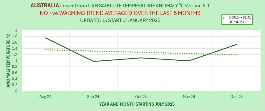
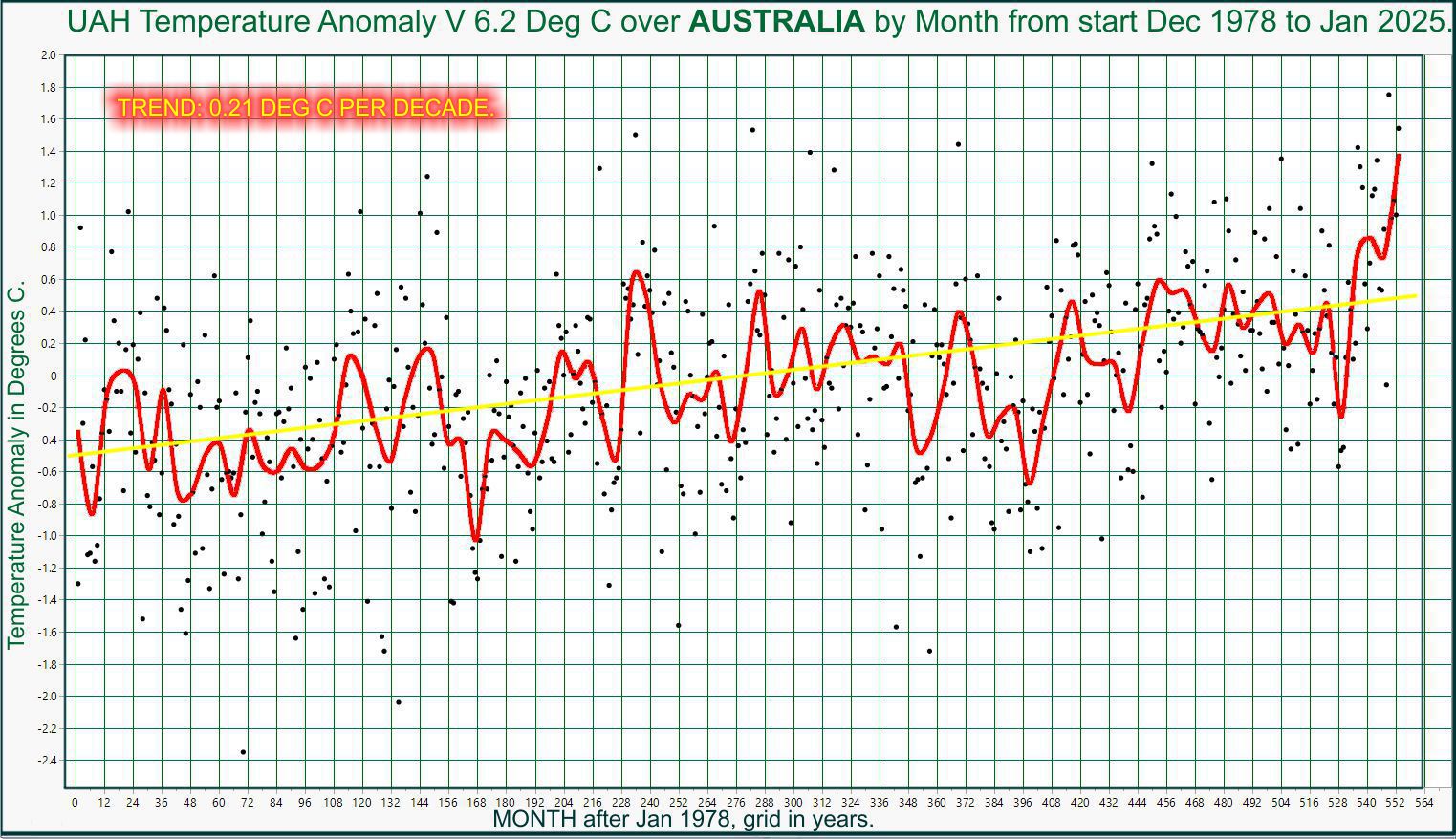
During 2024, there was a prominent high, positive temperature peak whose cause is still being researched. In some ways it has features unlike previous peak features.
A dominant peak like this ends any earlier pause, with the pause being defined in this monthly time series as the duration from the present, back to the month when the longest linear best fit always has a negative value, that it, it has been cooling since then, during the pause.
Because the present new pause that has now started lasts for only 5 months and will not grow faster than one month at a time for the time being, there is little point in continuing this calculation. I might revive it in 2 years if a pause seems to be developing.
Readers have requested a graph showing UAH anomaly temperatures over the Australian land mass since observations began.
Geoff S
Warmest year globally in WUWT’s beloved UAH.
Warmest year in the USA in WUWT’s beloved UAH.
No such thing as global warming?