From Dr. Roy Spencer’s Global Warming Blog
Roy W. Spencer, Ph. D.
The Version 6 global average lower tropospheric temperature (LT) anomaly for May, 2024 was +0.90 deg. C departure from the 1991-2020 mean, down from the record-high April, 2024 anomaly of +1.05 deg. C.

The linear warming trend since January, 1979 remains at +0.15 C/decade (+0.13 C/decade over the global-averaged oceans, and +0.20 C/decade over global-averaged land).
The following table lists various regional LT departures from the 30-year (1991-2020) average for the last 17 months (record highs are in red):
| YEAR | MO | GLOBE | NHEM. | SHEM. | TROPIC | USA48 | ARCTIC | AUST |
| 2023 | Jan | -0.04 | +0.05 | -0.13 | -0.38 | +0.12 | -0.12 | -0.50 |
| 2023 | Feb | +0.09 | +0.17 | +0.00 | -0.10 | +0.68 | -0.24 | -0.11 |
| 2023 | Mar | +0.20 | +0.24 | +0.17 | -0.13 | -1.43 | +0.17 | +0.40 |
| 2023 | Apr | +0.18 | +0.11 | +0.26 | -0.03 | -0.37 | +0.53 | +0.21 |
| 2023 | May | +0.37 | +0.30 | +0.44 | +0.40 | +0.57 | +0.66 | -0.09 |
| 2023 | June | +0.38 | +0.47 | +0.29 | +0.55 | -0.35 | +0.45 | +0.07 |
| 2023 | July | +0.64 | +0.73 | +0.56 | +0.88 | +0.53 | +0.91 | +1.44 |
| 2023 | Aug | +0.70 | +0.88 | +0.51 | +0.86 | +0.94 | +1.54 | +1.25 |
| 2023 | Sep | +0.90 | +0.94 | +0.86 | +0.93 | +0.40 | +1.13 | +1.17 |
| 2023 | Oct | +0.93 | +1.02 | +0.83 | +1.00 | +0.99 | +0.92 | +0.63 |
| 2023 | Nov | +0.91 | +1.01 | +0.82 | +1.03 | +0.65 | +1.16 | +0.42 |
| 2023 | Dec | +0.83 | +0.93 | +0.73 | +1.08 | +1.26 | +0.26 | +0.85 |
| 2024 | Jan | +0.86 | +1.06 | +0.66 | +1.27 | -0.05 | +0.40 | +1.18 |
| 2024 | Feb | +0.93 | +1.03 | +0.83 | +1.24 | +1.36 | +0.88 | +1.07 |
| 2024 | Mar | +0.95 | +1.02 | +0.88 | +1.35 | +0.23 | +1.10 | +1.29 |
| 2024 | Apr | +1.05 | +1.25 | +0.85 | +1.26 | +1.02 | +0.98 | +0.48 |
| 2024 | May | +0.90 | +0.97 | +0.83 | +1.31 | +0.37 | +0.38 | +0.45 |
The full UAH Global Temperature Report, along with the LT global gridpoint anomaly image for May, 2024, and a more detailed analysis by John Christy, should be available within the next several days here.
The monthly anomalies for various regions for the four deep layers we monitor from satellites will be available in the next several days:
Lower Troposphere:
http://vortex.nsstc.uah.edu/data/msu/v6.0/tlt/uahncdc_lt_6.0.txt
Mid-Troposphere:
http://vortex.nsstc.uah.edu/data/msu/v6.0/tmt/uahncdc_mt_6.0.txt
Tropopause:
http://vortex.nsstc.uah.edu/data/msu/v6.0/ttp/uahncdc_tp_6.0.txt
Lower Stratosphere:
http://vortex.nsstc.uah.edu/data/msu/v6.0/tls/uahncdc_ls_6.0.txt
i just got my lowest electric bill ever (kwh basis, 20 years this house) this may.
Nor Cal had a very cool April and May so my power bill was very low too.
Here is the Monckton Pause update for May. At its peak it lasted 107 months starting in 2014/06. Since 2014/06 the warming trend is now +0.34 C/decade.
Been a long drawn-out El Nino, hasn’t it.
No sign of any human causation, though.
Notice that all regions appeared to have cooled, apart from the Tropics (about 34% of the globe)
“Been a long drawn-out El Nino, hasn’t it.
No sign of any human causation, though.”
I wonder whether you actually do any reading outside of your own scribblings? No one and I mean no one, who has an IQ above 100, agrees with your silly “it was El Nino what done it” tantrums. And yet you continue to make a fool of yourself on a daily basis on this one. Keep doing it though. Just makes you look clueless.
Have another look at the chart and then tell me what the hell you’re talking about.
Look at the UAH data, simpleton.
Not even you are dumb enough to say there hasn’t been a lingering El Nino event that started May 2023…… or are you.
Don’t try to blame your deliberate ignorance on me.
Now.. do you have any evidence of human causation for this strong and extended El Nino event ??
Or are you just going to prattle on with deeply ignorant and blind zero-intelligence yappings.
Humans aren’t causing the El Ninos, we are causing the underlying trend that keeps making the El Ninos get warmer and warmer.
Unsupported assertions don’t become true just because you write them down.
Let me rephrase so that it is less offensive for you: Nobody is saying that humans are causing El Ninos, we are saying that the long term underlying trend, that keeps making the El Nino peaks get higher and higher, is caused by human activities.
Bnice demands evidence that the El Nino is caused by human activities, but no one has ever said it was. Do you agree with that?
El Nino peaks aren’t getting stronger. There were higher peaks in the past.
https://ggweather.com/enso/oni.htm
He’s talking about the global average temperature response to the El Ninos; not the El Ninos themselves.
Thank you, there is no observed trend in the strength of El Ninos. Something else is pushing the top of the El Nino peaks higher and higher, and it is the underlying long term warming trend.
Long term. 1957 was the start of the International Geophysical Year that addressed any of these questions. And they ALL decided satellite observation was needed to produce quality measurements, which didn’t start happening until 1979.
Bwhahahahahahaha, long term. Bwhahahahahahahahahahaha. Just a silly blip in time and he calls it “Long Term”
FYI:
The International Geophysical Year (IGY); also referred to as the third International Polar Year, was an international scientific project that lasted from 1 July 1957 to 31 December 1958
The origin of the International Geophysical Year can be traced to the International Polar Years held in 1882–1883, then in 1932–1933 and most recently from March 2007 to March 2009.
No, the warming comes ONLY at El Nino releases. UAH data shows that.
And still ZERO EVIDENCE .
Of course that’s true because ENSO is an emergent phenomenon that acts to cool the ocean. When the Pacific ventilates its accumulated heat into the atmosphere, although eventually it cools the overall ocean-atmosphere system, it warms the atmosphere. It takes time to then cool the atmosphere. If something is heating the oceans more than before, then by the time the ocean needs to ventilate again, the atmosphere is still at a warmer level and it just ratchets upward.
The question is why are the oceans warming?
The answer that AlanJ wants to believe is that CO2 emissions are enhancing the greenhouse effect, slowing the rate of cooling. That is consistent with evidence.
But he’s probably wrong or at best only partly right. It’s probably mostly that we’re pumping fewer aerosols into the air as the result of clean air regulations.
Either way, it’s the sun that warms the ocean. Aerosols prevent some warming, the enhancement of the GHE prevents some cooling.
Rephrasing doesn’t change the fact that you have totally zero evidence.
Actually, it highlights that you have absolutely ZERO evidence.
Los Ninos’ peaks aren’t getting higher and higher. All those between 1997-98 Super El Nino and 2015-16 Super El Nino were lower than 1997-98 peak. Super El Nino 2015-16 was fractionally warmer than 1997-98, but 2019-20 El Nino’s peak was lower. Now ending 2023-24 El Nino was boosted by the Tongan eruption, cleaner air (fewer SO2 cloud condensation nuclei) and nearing the height of a solar cycle, not by a bit more plant food in the air.
What I object to is claiming that humans are responsible for the “the long term underlying trend.” There is plenty of evidence that the anomalous seasonal ramp-up of CO2 is correlated with the heat of El Ninos, and the is plenty of evidence of anti-correlation between rising CO2 and temperatures.
You have no evidence of that.. You are talking fantasies as usual.
The trend between El Ninos is basically ZERO.
That is the result of superimposing a periodic curve atop a linear increasing trend. The El Niño peaks create a natural high point, after which you will measure lower slopes until the high point is reached or exceeded by the next El Niño. This does not impact the underlying long term trend. As scvblwxq has shown, the El Niños themselves are not getting stronger over time, their peaks are just being lofted ever higher by the warming trend.
El Nino’s are no more the cause of the recent warming than the tide is the cause of sea level rise. But don’t believe me…… Everyone here thinks Roy Spencer is an authority…. this is what he had to say only yesterday when a poster asked why things are so warm at the moment….
‘I can only speculate: Some combination of El Nino, Hunga Tonga (I’m skeptical of that), cleaner skies from less aerosol pollution, a decrease in cloudiness (measured by CERES) due to either positive cloud feedback on warming or some unknown mechanism, and increasing CO2 (which can’t explain a short-term peak, but can explain a tendency for each El Nino to be warmer than the last). And maybe some other influence we don’t know about?”
……”and increasing CO2 (which can’t explain a short-term peak but can explain a tendency for each El Nino to be warmer than the last.” I’d say that pretty much settles it. Unless, if you have some other authority who contradicts this, which I will be glad to read. But you don’t because you are barking up the wrong tree (ring). So I’m guessing you will now just resort to personal abuse. Your turn?
So, even Roy has just pure supposition.
Pure supposition IS NOT EVIDENCE.
“who has an IQ above 100″
So, more than twice what yours is !
There are not many people, or 3-toed-slothes, as simple as you. !
Don’t keep rising to it! Demeans you more than the other guy.
Please don’t presume to tell me what to do.
You aren’t a closet totalitarian leftist, are you !
I think that michel is giving you good advice. You are, of course, free to ignore it. However, you do so at the risk of reducing the influence of your comments in exchange for satisfying your ego.
We’re not telling you what you have to do. We’re trying to help you because you make climate realists look bad.
And you look lukewarmers look stupid.
Blimey mate! You are quite the rhetorical prodigy. How can I hope to restore a semblance of self-esteem after that withering takedown?
It’s not like green policies to backfire……
“Almost All Recent Global Warming Caused by Green Air Policies – Shock Revelation From NASA”
https://dailysceptic.org/2024/06/04/almost-all-recent-global-warming-caused-by-green-air-policies-shock-revelation-from-nasa/
Reduced emissions from ships didn’t stop the temperatures from cooling globally last month.
From the link: “The effect of the Hunga Tonga eruption continues to intrigue some scientists, although their curiosity is not reciprocated by the all-in mainstream CO2 promoters. Recently a team of Australian climatologists used the eruption, which increased the amount of water vapour in the stratosphere by up to 10%, as a ‘base case’ for further scientific work. Working out of the University of New South Wales, they reported that volcanoes blasting water vapour – a strong if short-lived ‘greenhouse’ gas – into the high atmosphere, “can have significant inputs on the climate system”. In fact they found that surface temperatures across large regions of the world could increase by over 1.5°C for several years, although some areas could cool by up to 1°C.”
Even Hunga Tonga didn’t stop the temperatures from cooling last month.
As always, there are more things in heaven and earth, than are dreamt of in our Climastrology.
Why do we approach this as a multiple choice test with only one factor involved? It’s A – Enhanced GHE; B – Reduced air pollution; C – Hunga Tonka stratospheric water vapor; …?
I suspect that it’s D – All of the above and more.
The water mass is slowly leaving the stratosphere, so cooling is not unexpected, as I commented last month. But the water is lessening slowly, so cooling is also liable to take time.
“No one and I mean no one, who has an IQ above 100″
Poor simpleton.. I doubt you even know anyone with an IQ greater than 100.
I appreciate your frustration with Simon. However, trying to insult him with a statement that is obviously unverifiable, and probably wrong, doesn’t give you any credence.
Yes, Simon is a stubborn guy who can be frustratingly wedded to his ideology. Who here isn’t?
I’m sure that the vast percentage of commenters here are intelligent enough. Many are so highly educated that they have nearly succeeded in eradicating their inborn common sense.
I would repeat that ad hominem abuse makes the abuser look bad and tarnishes the correct opinions of the abuser. Since there are a few opinions that I hold in common with bnice, chiefly that there is NO CLIMATE EMERGENCY, that tarnishes my opinions and gives me standing to complain.
Lost in the hooplah are two recent volcanic eruptions that have sent plumes of matter into the stratosphere: Tonga in January 2022 and Ruang in April 2024. The former ejected seawater and ash to a height of 58 km (190,000 ft) and the latter ash and sulfur dioxide to a height of 25 km (82,000 ft). Bear in mind that the Tambora eruption in 1815 resulted in Europe’s infamous “Year Without a Summer” some 18 months later.
After undersea Tonga eruption’s relatively small S load settled out, ending its mild cooling effect, the warming effect of 300 billion pounds of water injected into the usually dry stratosphere took over.
https://phys.org/news/2023-11-massive-eruption-stratosphere-chemistry-dynamics.html#:~:text=%22The%20Hunga%20Tonga%2DHunga%20Ha,first%20author%20of%20the%20paper.
This paper may already have been linked:
https://eos.org/articles/tonga-eruption-may-temporarily-push-earth-closer-to-1-5c-of-warming#:~:text=of%20Warming%20%2D%20Eos-,Tonga%20Eruption%20May%20Temporarily%20Push%20Earth%20Closer%20to%201.5%C2%B0,over%20the%20next%205%20years.
Ruang was more normal, with cooling from SO2 dominating.
The ups and downs in the graph correlate with peaks of El Ninos and valleys of La Ninas,
as shown in this article Image 7
https://www.windtaskforce.org/profiles/blogs/hunga-tonga-volcanic-eruption
https://www.windtaskforce.org/profiles/blogs/natural-forces-cause-periodic-global-warming
Since 1984 to 2024 (40 years) the warming trend increased the anomaly from
1984 -0.67°C to
2024 1.05°C
for a total difference increase of 1.72°C…hmmm
Sounds like we crossed the magical 1.5°C threshold considering its supposed to be 1.5°C above pre-industrial levels. Seeing that 1984 is certainly far warmer than pre-industrial 1850, that 1.5°C is more likely 2°C since 1850…or 1984 was cooler than pre industrial temperatures despite the CO2 load then…
So what happened???
Temperatures dropped somewhat..
No Tipping
No Runaway Hothouse
No perpetual drought
No biblical flooding
Guam is still upright
If by “1.5 C threshold” you mean as it is defined via IPCC SR15 section 1.2.1 pg 56 then understand that 1.5 C has not yet been crossed. And because of the way the definition works we don’t know the value for 1984 according to UAH because that would require data back to 1969 which does not exist. Similarly we do not yet know the value for 2024 because that requires data through 2039.
Given all the adjustments to the current temperature measurements as well as all the prior adjustments and adjusted adjustments and readjusted adjust ego the historical records…Does anyone really know what the real temperature is? Does anybody really care??
Yes. We know what the real temperature is within a reasonable margin of error. A lot of people care. Dr. Spencer and Dr. Christy, who produced this product, certainly care. I presume WUWT cares since they promote the product on the site.
Apparently the seething sarcasm wasn’t apparent enough
Yeah sorry. I always assume people want to have a serious discussion and my sarcasm detector is weak at best.
“ is weak at best.”
Like the rest of your mind
You missed the reference
https://youtu.be/b5ewTCEFUeY
You are right. I had no idea that song even existed until you posted it.
Still can’t understand that error is not uncertainty…
The 1.5C started as 2C , and was pulled from the nether regions of an AGW crackpot at the Potty factory.
It has absolutely zero scientific meaning.
But what about the new Monckton pause that started in April 2024? How long will it take before we get regular updates on that?
You make me sleepy……
UAH data shows that strong El Ninos nearly always break the near-zero trend that happens between them.
But those El Nino have nothing to do with anything humans have done.
Why do you need an update? It isn’t hard to compute. You CAN do it yourself can’t you?
But what about the global drop in temperature that just happened in May 2024?
Did the CO2 concentration control knob start decreasing?
As much as it can be satisfying to tweak the true believers like that, ultimately it isn’t effective in changing their minds.
Reality is that they are not so stupid as to believe something that can’t be explained logically and reconciled with the evidence. They are gullible enough or intellectually lazy enough to just accept the popular opinion.
In the CO2-is-master-control-knob theory, enhancing the greenhouse effect is the main leitmotif of Climastrology. It is the god steadily warming the climate. But like Zeus, CO2 is the king of the gods, but not the only god in the pantheon. Minor actors like aerosols from volcanoes and cargo ships can have transient effects.
There are myriad causes of ‘internal variability’ to explain away anything that casts doubt on the control knob theory.
If we want to persuade people that there is NO CLIMATE EMERGENCY, we need to recognize that their beliefs are consistent with the evidence. Many absolutely wrong explanations can be consistent with the evidence. Circumstantial evidence abounds, and cynically we might add, more is made up every day.
The UAH satellite temperature for the lower troposphere over Australia extends now to end of May 2024, a few days ago.
There has been no positive (warming) trend for the last 105 months, being 8 years and 9 months, calculated in the style of Viscount Monckton.
Despite unusual effects such as the large Hunga Tonga submarine volcano, the Australian picture differs from the global picture in visually significant ways. I have no idea about the physics or meteorology of this variation and there appears to be no shared scientific understanding yet, from those paid to study such matters.
Geoff S
I have notice that since 1998 Australia UAH tends to have an occasional spike, followed by cooling (hand drawn on this chart)
Can’t see how CO2 could do that.
Here’s the Australian Pause in context.
Red line is the trend across all the data, the blue line is the trend since September 2015.
Grey areas are the 95% confidence interval for the two trends, but as they are not corrected for auto correlation, they should be much bigger. But even without correction it’s clear that the underlying trend passes through the confidence interval for the pause, suggesting there is no significant change over the last 9 years.
.
And here’s what happens if you constrain the trend before and after September 2015 so they are continuous. No significant change, but if anything a slight acceleration since 2015.
“calculated in the style of Viscount Monckton.”
i.e. cherry-piclinh a start date, and ignoring the large uncertainty in the trend.
Yawn…
No he DOES NOT cherry-pick the start point..
You really are dumb if you STILL haven’t figured that out !
At zero trend, the uncertainty is equal in both + and – direction.
The large uncertainty (actually unknown uncertainty) is a result of climatologists rarely specifying the uncertainty range, and that includes Roy.
UAH: [Christy et al. 2003]
RSS: [Mears et al. 2011]
BEST: [Rohde et al. 2013]
GISS: [Lenssen et al. 2019]
HadCRUT: [Morice et al. 2020]
NOAA: [Huang et al. 2020]
On e again, the uncertainty is mostly not caused by uncertainty in the measurements. It’s the result of natural variability in the global temperature caused by a variety of factors, including ENSO.
You still haven’t figured out measurement uncertainty.
Natural variation is *NOT* measurement uncertainty. Measurement uncertainty is *NOT* natural variation.
The measurement of natural variation is conditioned by the measurement uncertainty that goes with the measurement.
If you have two stated values, 3 and 4, what is the variation? 1? If the measurement uncertainty of each is 0.5 then what is the natural variation (give both the stated value and the associated measurement uncertainty).
Indeed, much of the statistical manipulation of data is with sets that don’t meet the requirement of ‘stationarity’ — an unchanging mean and SD with time.
That’s how calculating the uncertainty of a trend works. A 1000 basic text books will explain it. There’s a straight forward equation based on assumptions that there is a trend with random independent error. Then there’s more advanced techniques to do with auto correlation and such like.
Calling it statistical manipulation is rich coming from someone defending looking at every possible starting point until they find the one that gives the longest zero trend. Looking at the uncertainty if the trend is one way of checking you are not fooling yourself.
Then there are two components to the uncertainty: 1) The approximately random variation of the de-trended measurements, and 2) the uncertainty in the slope of the trend, which is suggested by the r^2 value, which explains the percentage of variance in the dependent variable.
I wouldn’t regard r² as a measure of uncertainty. It’s a measure of how much variation can be explained by the independent variables. If you are talking about a period with a zero trend, the r² will always be zero.
The 2nd tells you nothing about the accuracy of the data points being used to evaluate the r^2 value. The slope of the trend line has to be conditioned by the measurement uncertainty of the data points. The measurement uncertainty simply can’t be ignored as bellman and climate science does.
Even in 1) the random variation has to be conditioned by the measurement uncertainty of the data points used to establish the variation (I am assuming you are talking about the standard deviation). The uncertainty in the minimum and maximum values in the data set change the variance calculated for the data set using only the stated values and *increases* the amount of variation (i.e. the standard deviation).
You simply can’t just ignore measurement uncertainty in anything to do with measured values. Garbage in, garbage out.
That is an odd criticism considering that I’m hardly known for being a defender of worrying about the length of time of a hiatus.
Sorry if I incorrectly implied you were one of the pause faithful. There are so many here with axes to grind, it’s difficult to keep track.
“That’s how calculating the uncertainty of a trend works. “
The uncertainty of a trend line HAS to be conditioned by the measurement uncertainty of the data used to find the best-fit trend line. Climate science doesn’t do that. You and climate science just assume all stated values are 100% accurate because you assume all measurement uncertainty is random, Gaussian, and cancels.
The proof is that you didn’t answer the question I posed to you.
You continually deny you assume all measurement uncertainty is random, Gaussian, and cancels yet here you are claiming “assumptions that there is a trend with random independent error”
You’ve been given multiple examples showing that you simply cannot assume all measurement uncertainty is random, Gaussian, and cancels. Electronic components typically don’t age and change in a random manner. Resistors that depend on the density of materials typically drift in the same direction as they suffer long-term heating, capacitors as well. And it doesn’t matter if they are discrete components or formed on a substrate. Even the glass in LIG thermometers will change in the same manner over time. Glass in one doesn’t shrink as it distorts under extended heat while the glass in another one will expand!
You and climate science have never accepted the international standards that measurement uncertainty adds – ALWAYS. That’s why you either do direct addition of the absolute vale of the measurement uncertainty or you do root-sum-square addition. You don’t add some of the uncertainty values and subtract others so it all comes out to 0 (zero).
If the measurement data points are uncertain then so is the trend line. Unless the segment difference is outside the measurement uncertainty interval you can’t even know if the trend is negative or positive. It simply doesn’t matter what the best-fit metric is from assuming all measurement uncertainty is 0 (zero) – that’s doing nothing but fooling yourself. And as Fyenman pointed out, yourself is the easiest person to fool.
HAS to you say? So why did you never critizise Monkton or sherro01 for not doing it? You were the one insisting there was zero uncertainty in Monckton’s determination if the exact month the pause started.
I’ll ignore your usual lies about what I believe.
“The proof is that you didn’t answer the question I posed to you.”
I’m on holiday.I’m not obliged to help you with your homework, especially when it’s your usual toy examples that have nothing to do with the uncertainty of a trend.
But if you mean the one about the difference between 4 and 3. The answer is 1, and if both are measurements with an assumed independent random standard uncertainty of 0.5, the uncertainty of the difference is 0.5 × √2.
If they are entirely dependent uncertainties the uncertainty of the difference reduces to 0.
“HAS to you say? So why did you never critizise Monkton or sherro01 for not doing it? You were the one insisting there was zero uncertainty in Monckton’s determination if the exact month the pause started.”
Your memory is failing. You don’t even remember me telling you that I don’t believe in UAH trends because of the measurement uncertainty associated with the satellite readings being converted to temperature!
As Willis has tried to point out you use the data you are presented with when discussing conclusions.
“I’ll ignore your usual lies about what I believe.”
No lies. I quoted your exact words. ““assumptions that there is a trend with random independent error””
You *do* assume all measurement uncertainty is totally random, Gaussian, and cancels. You can deny it all you want but, as I keep telling you, it comes through in every thing you do.
“But if you mean the one about the difference between 4 and 3. The answer is 1, and if both are measurements with an assumed independent random standard uncertainty of 0.5, the uncertainty of the difference is 0.5 × √2.”
You are *still* avoiding the issue. The uncertainty becomes a direct addition, not a root-sum-square addition. Root-sum-square applies if you assume some of the uncertainty cancels. It is a *best* case uncertainty. Direct addition is a “worst” case uncertainty. Both mean that you can’t know what the “true value” of the slope is.
If you can’t know what the “true value” of the slope is then you can’t know what the “best-fit” linear regression line actually and that, in turn, means you can’t know what the best-fit metric is either! Your “uncertainty of the trend” depends solely on your ubiquitous assumption that all measurement uncertainty is random, Gaussian, and cancels.
“No lies. I quoted your exact words. ““assumptions that there is a trend with random independent error”””
And ignored the context. Quote the entire sentence.”There’s a straight forward equation based on assumptions that there is a trend with random independent error.”
The simple equation, as explained by Taylor, is based on those assumptions. That does not mean those assumptions are correct, or that you cannot use different assumptions. If you’d ever paid any attention, you would know that the assumption of independence is not correct in cases like this, and that is why I say the uncertainties will be bigger – you have to account for auto-correlation.
You can make the models as complicated as you like – assume non-Gaussian distributions, assume the distributions change over time, assume errors in the measurements.
You keep jumping from the concept of a simplifying assumption, to claiming that everyone believes those assumptions are always correct.
“You don’t even remember me telling you that I don’t believe in UAH trends because of the measurement uncertainty associated with the satellite readings being converted to temperature!”
You are correct, – I have no memory of you telling Monckton you didn’t believe his pause becasue of the huge measurement uncertainty in his preferred data set. On the contrary, I remember you attacking me for daring to suggest there was any uncertainty in the trend.
“You are *still* avoiding the issue.”
I’m not a psychiatrist – I can’t help you with your issues. If you have something to say, than say it, instead of playing these stupid games. We are not talking about the difference between two values – we are talking about a least squares regression through 100 different data points.
“If you can’t know what the “true value” of the slope is then you can’t know what the “best-fit” linear regression line actually and that, in turn, means you can’t know what the best-fit metric is either!”
Gibberish and wrong. You don’t need to know the true slope to know what the best fit is – that’s exactly what the equations for the linear regression give you. The best fit to the data – defined in this case by the line that minimizes the square of the residuals. You should know that, having studied Taylor so completely.
“Your “uncertainty of the trend” depends solely on your ubiquitous assumption that all measurement uncertainty is random, Gaussian, and cancels.”
Still waiting for you to tell me if you think my uncertainty is too big or too small. You could simply take the Australian data and show what you think the correct uncertainty should be – then we can see if you still agree with me that the uncertainty means there is no significant difference between the short term pause, and the long term trend.
“ I have no memory of you telling Monckton you didn’t believe his pause becasue of the huge measurement uncertainty in his preferred data set.”
Your lack of reading comprehension is showing again. The pause DOES exist in the data he is using – the same data climate science uses. So you have two choices, 1. if CoM is wrong then so is climate science or 2. that it is impossible to know what is happening.
“I remember you attacking me for daring to suggest there was any uncertainty in the trend.”
Your memory skills are as bad as your reading comprehension skills.
What I have *always* said, and which you seem to be unable to comprehend because of your lack of reading comprehension ability, is that what is happening is part of the GREAT UNKNOWN. The data has such inherent measurement uncertainty that it is impossible to identify temp differences less than the units digit. That makes knowing the actual trend of the “global temp” impossible to know. It’s part of the GREAT UNKNOWN.
As usual your cognitive dissonance is right at the forefront. You want your cake and to eat it too and so you say whatever you have to in the moment. As I said, you have two choices, either CoM’s pause is correct and climate science can calculate anomalies in the hundredths digit or CoM’s pause is unknowable and climate science can *NOT* calculate anomalies in the hundredths digit and their conclusions are unknowable garbage.
Pick one and stick with it!
“We are not talking about the difference between two values – we are talking about a least squares regression through 100 different data points.”
Why do you ALWAYS make such idiotic assertions? The slope of a linear regression line DEFINES the difference between two consecutive values on the line! The slope of that line is based on minimizing the residuals between the given measurements and the line (the difference between two values)!
“You don’t need to know the true slope to know what the best fit is”
But the best-fit metric depends on the values of the data, including their measurement uncertainty! There simply is no true value for the best-fit metric if there is no true value for the data points!
You keep getting stuck in the paradigm of measurements being “true value +/- error” that the international community abandoned 50 years ago. You simply can’t let that paradigm go because in your statistics training all data is 100% accurate. So you just ignore the uncertainty of the data. You were never taught how to integrate data uncertainty into statistical analysis and you stubbornly refuse to learn how to do it today! Instead you just claim that sources like the GUM, Taylor, Bevington, and Possolo are all wrong. You can’t admit, even to yourself, that Possolo in TN1900, Ex 2, had to assume that all measurements were 100% accurate with no measurement uncertainty. For you, making that assumption is just standard practice for *everything*. Right down to stating that you *can* find the “true value” of the slope of a linear-regression line for a set of measurements. And then you want to turn around and claim that CoM can’t do the same thing!
“Still waiting for you to tell me if you think my uncertainty is too big or too small.”
It’s neither. You just assume it’s always ZERO!
The measurement uncertainty over time for *any* set of temperature data is at least in the units digit because that is how the data has been recorded. Even in the current NWS ASOS system the temperature is recorded by rounding the measurement to the nearest units digit in Fahrenheit and then converting to Celsius in the tenths digit. That alone introduces measurement uncertainty that will be in the units digit, quoting the Celsius value in the tenths digit is is adding resolution that you simply can’t know!
“then we can see if you still agree with me that the uncertainty means there is no significant difference between the short term pause, and the long term trend.”
There is no significant difference BECAUSE YOU CAN’T KNOW EITHER ONE IN ORDER TO COMPARE THEM!
The real nuts-and-bolts issue he’ll never acknowledge.
He is so brainwashed by the antiquated meme of “true value +/- error” that he believes the treatment of measurements and measurement uncertainty in the GUM is wrong. It all comes back to the basic meme of “all measurement uncertainty is random, Gaussian, and cancels”. Therefore random sampling as in an MC simulation can tell you the “true value”.
They are 50 years out of date and can’t admit it.
Yep!
Point to a single time when I’ve said the GUM is wrong. It’s strange how you can say this, yet at the same time admire Pat Frank who clearly said the GUM is wrong, and accused me of worshiping the GUM.
The worst I’ve said about the GUM is that some of it’s language is a bit hand wavy and has clearly confused some people here. E.g. all the claims about what “could be reasonably attributed to the measurand” actually means.
“It all comes back to the basic meme of “all measurement uncertainty is random, Gaussian, and cancels”.”
Is that what you think? Why have you never mentioned it before?
“Therefore random sampling as in an MC simulation can tell you the “true value”.”
You are caught in a mental loop. It doesn’t matter how many times I explain why that is wrong your brain just flips a bit and you read the exact opposite. But I’ll state it again, just in case there’s a glimmer of hope it will penetrate your reality distortion field – you cannot find the true value of anything – that’s why it’s uncertain. The point of an MC simulation is not to find a single correct result or true value. The purpose is to estimate the uncertainty of any result. Uncertainty does not mean you know the true value – it means you do not know the true value. They are mutually incompatible things. If the result is uncertain then you do not know it’s a true result, and if you did know it was the true result there would be no uncertainty.
Did any of that make sense to you?
“They are 50 years out of date and can’t admit it.”
The second edition of Taylor’s book on error analysis came out in 1996. Did he know it was 20 years out of date by then?
It wasn’t out of date. His original book was pioneering in changing metrology from the meme of “true value +/- error” to “stated value +/- uncertainty”.
His copyright is 1982 and 1997.
As usual you are cherry picking without reading for meaning. If you would read his preface to the second addition you would find that he didn’t change anything in his approach to “stated value +/- uncertainty”.
It all makes sense. But it doesn’t explain why you always assume that measurement uncertainty is random, Gaussian, and cancels in everything you assert!
Taylor, Bevington, and Possolo all tell you that systematic uncertainty is not amenable to statistical analysis.
An MC is a statistical analysis – it can’t identify or estimate systematic uncertainty. It can only look at random uncertainty.
So your belief that an MC can somehow help you determine measurement uncertainty is – as always with you — based on your meme that all measurement uncertainty is random, Gaussian, and cancels.
“So you have two choices”
Oh, the false dilemma fallacy. I choose 3. UAH data, whilst far from perfect, is assumed to be reasonably accurate by most here, but Monckton seriously misuses statistics in his claims.
“The slope of a linear regression line DEFINES the difference between two consecutive values on the line!”
How on earth does kit do that? At best it predicts the mean value for the dependent variable at a specific point.
“The slope of that line is based on minimizing the residuals between the given measurements and the line”
The squares of the residuals.
“(the difference between two values)”
Did you spot your own swerve there? You started by talking about the difference between consecutive points, and now you are talking about the difference between a predicted and the actual value.
“You keep getting stuck in the paradigm of measurements being “true value +/- error” that the international community abandoned 50 years ago.”
Did they? Coming from someone who is happy to redefine the meaning of Gaussian, it’s a bit odd to here you insist on following what the international community says. Even odder when you also say I’;m not allowed to disagree with Taylor and Bevington, who use exactly that paradigm.
Your problem though is whatever paradigm is actually used makes no difference to the calculations – you still use the equations derived from the error model, whatever language you choose to use.
“You simply can’t let that paradigm go because in your statistics training all data is 100% accurate. ”
This from someone who likes to bandy phrases like cognitive dissonance around. How can saying that all values have an error term, possible equate to believing all data is 100% accurate?
“Instead you just claim that sources like the GUM, Taylor, Bevington, and Possolo are all wrong.”
You’ve just claimed Taylor and Bevington are wrong for using the error paradigm. I have never said that any of those sources are all wrong. I can;t think of many examples where they are wrong at all.
“You can’t admit, even to yourself, that Possolo in TN1900, Ex 2, had to assume that all measurements were 100% accurate with no measurement uncertainty.”
Follow your logic – first you attack me for saying Possolo is wrong, then you say I’m wrong for assuming there is no measurement uncertainty, and now you are claiming Possolo made the same assumption I made. Do you not see the contradictions?
“Right down to stating that you *can* find the “true value” of the slope of a linear-regression line for a set of measurements.”
I’ve stated, repeatedly, that you cannot find the true slope of a linear regression. That’s one of my objections to the pause, remember?
“It’s neither. You just assume it’s always ZERO! ”
You lies are getting quite pathetic. I literally started this discussion by saying there were large uncertainties, yet you want to pretend I said there was zero uncertainty.
“Oh, the false dilemma fallacy. I choose 3. UAH data, whilst far from perfect, is assumed to be reasonably accurate by most here, but Monckton seriously misuses statistics in his claims.”
You are back to wanting your cake and to eat it too. CoM does *not* misuse statistics and you’ve never been able to show such. And no one knows the accuracy of UAH. I’ve never seen a complete measurement uncertainty budget for UAH. Certainly clouds and water vapor affect its readings, is sampling is far from perfect, and the conversion algorithm has built in uncertainty.
“How on earth does kit do that? At best it predicts the mean value for the dependent variable at a specific point.”
OMG! A linear regression line is of the form y = mx + b. If I give you an “x” value, the y (y1) value can be calculated. If I then give the next x value in sequence you can calculate the y (y2) value for that x. The difference is y2 – y1!
” Even odder when you also say I’;m not allowed to disagree with Taylor and Bevington, who use exactly that paradigm.”
Neither of them use that paradigm. This only shows that you have never read either one for meaning, only for cherry picking purposes. The title of Section 1.2 in Bevington is “UNCERTAINTIES”.
“The term error suggests a deviation from the result of sme “true” value. Usually we cannot know what the true value is, and can only estimate the errors inherent in the experiment. If we repeat an experiment, the results may well differ from those of the first attempt. We express this difference as a discrepancy between two results. Discrepancies arise because we can determine a result only with a given uncertainty.” (tpg, italics are in the text)
It simply doesn’t matter how often all of this is pointed out to you. You’ll never get it because you are so invested in your memes of “true value +/- error” and “all measurement uncertainty is random, Gaussian, and cancels” that you are simply unable to fight your way out of that paper bag you are trapped in.
“CoM does *not* misuse statistics”
Hilarious.
You’ve spent far more time than is healthy berating me for underestimating the uncertainty of the pause – yet your hero worship makes you blind to the fact that Monckton doesn’t even mention uncertainty.
“OMG! A linear regression line is of the form y = mx + b. If I give you an “x” value, the y (y1) value can be calculated. If I then give the next x value in sequence you can calculate the y (y2) value for that x. The difference is y2 – y1!”
Please at least try to understand the points you are responding to. The linear regression is giving you the best fir of the data not the actual values. It represents the mean value of y for a given x, not the actual value. Your claim that it defines the difference between consecutive values is wrong, unless you have an entirely deterministic relationship between x and y.
“Neither of them use that paradigm.”
Then you are going to have to say exactly what paradigm you are talking about. You keep yelling uncertainty is not error, yet both of your recommended books are explicitly about error analysis, and how it relates to uncertainty. They are all based on the model that a measured value is equal to a true value plus an error. and that the extent of the possible errors defines the size of the uncertainty. Your quote from Bevington is saying just that.
He states it in the summary:
…
“yet your hero worship makes you blind to the fact that Monckton doesn’t even mention uncertainty.”
Neither does UAH mention measurement uncertainty, only the SEM. As willis tried to point out to someone (was it you?), you use the data you are given when making a point. You don’t just make it up as you go along the way you do.
“Please at least try to understand the points you are responding to. The linear regression is giving you the best fir of the data not the actual values”
In order to calculate a residual you need two values. It is the residuals that determine the best fit. One of the values is the given data point. The other is the corresponding point on the regression line.
You can’t even get this simple math right!
“Then you are going to have to say exactly what paradigm you are talking about.”
bellman: “You’ve just claimed Taylor and Bevington are wrong for using the error paradigm”
I gave you both the Bevington quote to show you that NEITHER use the “true value +/- error” paradigm.
Here it is one more time!
““The term error suggests a deviation from the result of sme “true” value. Usually we cannot know what the true value is, and can only estimate the errors inherent in the experiment. If we repeat an experiment, the results may well differ from those of the first attempt. We express this difference as a discrepancy between two results. Discrepancies arise because we can determine a result only with a given uncertainty.” (tpg, italics are in the text)”
How many more times will you refuse to actually READ and COMPREHEND what Taylor, Bevington, and the rest are telling you?
Again: “Discrepancies arise because we can determine a result only with a given uncertainty.””
*YOU* are the one stuck in the “true value +/- error” paradigm, not Taylor, Bevington, or any of the other metrology experts.
“And ignored the context. Quote the entire sentence.”There’s a straight forward equation based on assumptions that there is a trend with random independent error.””
So what? You are still saying you assumed all measurement uncertainty is random, Gaussian, and cancels! What else is “random independent error”? BTW, because of measurement uncertainty the “ERROR” is impossible to know unless you know the “true value”. Do *YOU* know the true value?
“The simple equation, as explained by Taylor, is based on those assumptions.”
Once again, you have *NEVER*, not once studied Taylor in order to understand what is he doing. You’ve never done the examples in order to learn something.
Taylor’s equations in Chapter 3 assume PARTIAL cancellation, not complete cancellation. *YOU ARE ASSUMING COMPLETE CANCELLATION*. I.e. random, Gaussian, and cancels.
” If you’d ever paid any attention, you would know that the assumption of independence is not correct in cases like this”
It’s not the assumption of independence, it is assuming that all measurement uncertainty is random, Gaussian, and cancels!
“You keep jumping from the concept of a simplifying assumption”
This is the excuse of a blackboard mathematician/statistician who doesn’t care about whether the assumptions mean anything in the real world!
“to claiming that everyone believes those assumptions are always correct.”
When you make the assumption EVERY SINGLE TIME that all measurement uncertainty is random, Gaussian, and cancels it’s pretty damn hard to do anything other than assume you believe that assumption is always correct!
“So what? You are still saying you assumed all measurement uncertainty is random, Gaussian, and cancels!”
Your lie, repeated ad nauseam, is that I always assume those things. I do not. Pointing out that the standard equation, as described by Taylor, makes those assumptions does not mean that I always assume them. As I say, you need to understand the difference between simplifying assumptions, and personal beliefs.
“Do *YOU* know the true value?”
What bit of “no, because it’s uncertain” do you not understand?
“Once again, you have *NEVER*, not once studied Taylor in order to understand what is he doing.”
Impending irony alert.
“Taylor’s equations in Chapter 3 assume PARTIAL cancellation, not complete cancellation.”
I’m talking about chapter 8 – you know, the one about linear regression.
“ I do not.”
Of course you do. Like when you say the standard deviation of the stated values can be used to determine measurement uncertainty. You can only do so by assuming measurement uncertainty is 0 (zero). You can only assume it is zero if you assume it is random, Gaussian, and cancels. Just as Possolo did in TN1900, Ex. 2!
You *always* assume measurement uncertainty is random, Gaussian, and cancels in every thing you do. EVERY SINGLE TIME. Apparently you don’t even realize that do.
Taylor and Chapter 8? You are cherry picking again! You didn’t understand anything Taylor says in Chapter 8. You didn’t even look at Fig 8.1(b)!
In Chapter 8 Taylor is trying to find out if the relationship between x& y is linear. He says: “The second question that must be asked is whether the measured values (x1,y1), …, (xn,yn) do really bear out our expectation that y is linear in x.”
No where in Section 8 does he state what the linear relationship *is*, i.e. the *true value* of the slope of the linear line, only that if it is within the error bars that it can then judge visually if the relationship is linear.
Note that in Section 8.2 (finding constants A and B) he says:
“If we knew the constants A and B the, for any given value of x_i (which we are assuming has no uncertainty), we could compute the true value of the corresponding y_i, …”
“The measurement of y_i is governed by a normal distribution centered on this true value, with a width parameter of σ_y.” (tpg note: normally distributed implies random uncertainty only)
“In the now familiar way, we will assume that the best estimates for the unknown constants A and B, based on the given measurments, are those values of A and B for which the probability Prob_A,B(y1, …, yn) is maximum …”
————————————–
As I said, you are CHERRY-PICKING again.
In Section 8.3, Uncertainty in the Measurements of y:
“Remember that the numbers y1, …,, yn are not N measurements of the same quantity. … Thus we certainly do not get an idea of their reliability by examining the spread in their values.”
“Nevertheless, we can easily estimate the uncertainty σ_y in the numbers y1, …, yn. The measurement of each y_i is (we are assuming) normally distributed about its true value A +Bx_i with a width parameter σ_y”
As Taylor stated in Chapter 4, most of the rest of the book assumes random uncertainty only, no systematic uncertainty. That is certainly the case in Chapter 8. That’s what the words “normally distributed about its true value” means!
Someday you *really* need to stop cherry-picking stuff hoping it will validate you misunderstandings about measurement uncertainty!
Rule 1: Measurement uncertainty in field applications cannot be assumed to be “normally distributed” when you are measuring different things using different things.
Rule 2: Measurement uncertainty always grows, you can’t reduce it through averaging.
Rule 3: Systematic uncertainty is not amenable to statistical analysis.
Resign yourself to this and maybe you’ll see some light on the subject.
Not a single one of those basic textbooks give the data points in the form of “stated value +/- measurement uncertainty”. It’s always “stated value” only.
He will never figure it out.
Once again, I am talking about the uncertainty if the trend. Not measurement uncertainty.
For a zero trend, the uncertainty is equal either side.
Your mathematical understanding is really the pits, isn’t it.
“For a zero trend, the uncertainty is equal either side.”
Correct.
Now if only you could examine the consequences of that uncertainty, rather than resorting to your usual Ad Homs. If you want to demonstrate my lack of mathematical understanding, try discussing the significance of this claimed pause using statistics rather than insults.
You lack of math understanding is demonstrated by your continued dependence on the meme of “all measurement uncertainty is random, Gaussian, and cancels” so that you can ignore it.
Yet again I’m told I lack mathematical understanding, by someone who in the past few years has insisted that standard deviations can be negative, rectangular distributions are Gaussian, square waves are sinusoidal, and Monte Carlo methods do not use ran dom sampling.
It should go without saying that he then lies about what I believe, despite me repeatedly explaining it to him.
…and who conflates sums with averages, thinks addition (+) is interchangeable with division (/), and that the derivative of x/n is 1. So yeah, it almost defies credulity that you are being lectured on mathematical understanding from someone who’s understanding is remedial enough that it lags behind even elementary school children in some cases.
The MEASUREMENT UNCERTAINTY is the propagated measurement uncertainty of the data points in the population or sample.
It is *NOT* the standard deviation of the sample means.
Nor is the derivative of x/n = 1. I’ve never said that. Once again, you and bellman have *NEVER* figured out relative uncertainty and how the power of a factor becomes a weighting factor. As laid out in Taylor, when you to multiplication or division you use RELATIVE MEASUREMENT UNCERTAINTY, just as Possolo did in his example of the measurement uncertainty in the volume of a barrel. A squared factor, e.g. R^2, gets a weighting factor of 2 in relative uncertainty. The partial derivative of R^2 is not just 2 yet that is what Possolo came up with for the relative uncertainty factor of u(R).
Neither of you have figured this one out yet.
Look at Taylor Eq. 3.26, the uncertainty is a power.
if q = x^2 then
u(q)/q = 2 (u(x)/x)
The power becomes a weighting factor!
Neither of you understand calculus or even basic algebra worth a tinkers dam.
Nothing you ever assert makes any physical sense at all. You are either saying what you need to say in the moment or you are displaying cognitive dissonance.
Just keep digging. Your ability to misinderstand so many concepts whilst lecturing others on their mathematical knowledge is truly staggering.
1. You still don’t understand that being able to subtract a value does not mean that value is negative.
2. OK Humpty Dumpty, use words to mean whatever you want them to mean, but don’t expect others to go along with your alternative definitions. And don’t lecture others whilst continuing to misuse standard terminology.
3. Complete gibberish, which just shows you still don’t understand how MC works, and still doesn’t address the fact that you were claiming MC doesn”t use random sampling.
Just keep digging. You are really demonstrating how easily you can fool yourself. Remember – you are the easiest person to fool, and the best demonstration of that is your inability to even consider you might have got something wrong. Added to that your believe that writing things in
all caps proves your point, and constantly diverting from the subject.
“You *do* want us to believe the CLT applies in one case but not in another one”
The CLT applies to any case where your sample is from IID distributions.
“…you don’t believe sampling of even a skewed distribution can result in a Gaussian distribution of the sample means”
Speaking of “Unfrekaingbelievable”, how long did I have to keep pointing this out to you and Jim, whilst you insisted that the CLT only applied to Gaussian distributions?
What you seem to not realize is that the CLT does not mean that the sampling distribution from a non-Gaussian distribution will be Gaussian. What it says is that the sampling distribution will tend to a Gaussian distribution as sample size increases. This is one area where an MC evaluation is useful. If your distribution is not at all Gaussian, and / or, your sample size is small, it can give you a better estimate than the approximation you get from assuming a Gaussian distribution.
You’ll never get it, will you?
1.Standard deviation of the stated values will ONLY give you the measurement uncertainty IF AND ONLY IF you assume all measurement uncertainty is random, Gaussian, and cancels.
Why do you think Possolo assumed all measurement uncertainty was 0 (zero) in TN1900, EX 2?
It was so he wouldn’t have to condition the standard deviation of the stated values by a measurement uncertainty value!
No.2: I have told you repeatedly that when I say Gaussian that is to indicate a symmetric distribution. Your memory is *YOUR* problem, not mine.
The CLT does *NOT* only apply to Gaussian distributions. It applies to *ANY* distribution, be it Gaussian or skewed. No one has ever disputed this. The issue is that the CLT doesn’t help with statistical analysis of a skewed or multi-modal distribution where the average and the median are different. You can’t seem to get that into your head no matter how many times you are told it.
“What it says is that the sampling distribution will tend to a Gaussian distribution as sample size increases.”
And what does that Gaussian distribution of sample means imply for a non-Gaussian parent distribution? Ans: Very litle, certainly *not* the accuracy of the mean!
You keep trying to rationalize to yourself that you can somehow decrease measurement uncertainty merely by assuming it is all random, Gaussian, and cancels.
You can’t. Resign yourself to that.
Twist, twist and twist. All this this because I pointed out that you think standard deviations can be negative, that rectangular distributions were Gaussian and that Monte Carlo methods did not involve random sampling.
You are really demonstrating how unfit you are to lecture others on their understanding.
Nothing you say in 1 – has anything to do with the point. Just admit that you did think standard deviations could be negative, and say whether you still think that is the case. But you ignore that and try to drag this into more idiotic claims. Are you now saying that the GUM is wrong to define standard uncertainty in terms of the standard deviation? And why keep lying about TN1900?
And you just keep digging about Gaussian distributions. You still don’t get that the claim that you’ve repeatedly used the term Gaussian to mean all symmetric distributions – is the point. It doesn’t matter how many times you’ve claimed it you are still wrong.
And whatever point you think you are making for 3, it has nothing to do with whether you still think that MC methods do not use random sampling.
The uncertainty of the trend *IS* also conditioned by the measurement uncertainty of the data points used to determine the trend. A fact you stubbornly refuse to admit.
A trend line is made up of segments between adjacent data points. If those adjacent data points are uncertain then so is the slope of the line between the two adjacent data points. A linear slope is nothing more than finding a line with a common slope for each segment. But if the slope of the line between the segments is uncertain then so will the linear line with a common slope.
You “uncertainty of the trend” is nothing more than the best fit to the stated values of the data points while ignoring the measurement uncertainty of the data points. A common tactic in climate science. “All measurement uncertainty is random, Gaussian, and cancels”
The slope of that linear line with a common slope is just as uncertain as the measurement uncertainty of the individual data points.
“A trend line is made up of segments between adjacent data points”
Er, no. That would just be a wibbly wobbly line.
The trend line we are talking about us the line that minimises the total squares of the residuals – hence the method of Least Squares.
Here’s the question for you. I’ve asked it many times before so I don’t expect an answer. When you do your calculation of the uncertainty of the trend, taking in all the uncertainties and systematic errors in UAH, do you expect it to be bigger or smaller than what I would estimate ignoring all those uncertainties?
I ask because my point was that there are large uncertainties in the pause trend and that means there is not enough evidence to demonstrate any significant change. If you want to suggest the uncertainty is even greater, that doesn’t help your cause.
“Er, no. That would just be a wibbly wobbly line.”
YES! A linear regression is just a way to straighten out the wobbly line!
But it is the segment to segment differences that determine what the linear regression will be!
“Here’s the question for you. I’ve asked it many times before so I don’t expect an answer. When you do your calculation of the uncertainty of the trend, taking in all the uncertainties and systematic errors in UAH, do you expect it to be bigger or smaller than what I would estimate ignoring all those uncertainties?”
The problem is not that you haven’t been answered. The problem is that you won’t accept the answer because of your dogmatic belief that all measurement uncertainty is random, Gaussian, and cancels.
The “uncertainty of the trend” is ONLY A METRIC FOR HOW THE LINE FITS THE STATED VALUES!
You *still* don’t understand measurement uncertainty! The problem is that the TRUE trend line is part of the GREAT UNKNOWN!
If you had answered my previous question concerning what the trend line between 3 +/- 0.5 and 4 +/- 0.5 actually is you might get a glimmer of understanding. Instead you just ignore it because it doesn’t fit your dogma.
The actual trend line could be anywhere in the universe of 2.5 to 4.5 and 3.5 to 3.5. Or a slope somewhere between 0 and 2. What it actually is just can’t be determined!
*YOU* would answer that the slope of the trend line is 1. And the R^2 value is 1. Perfect fit. All residuals = 0. An uncertainty of 0.
So your “uncertainty of the trend line” is *far bigger than what you would calculate! The uncertainty becomes a +/-1 from an individual uncertainty of +/- 0.5. A direct addition of the measurement uncertainty. And totally different from your “uncertainty of the trend line” equaling zero.
When you change each individual data point to its possible reasonable value plus/minus then the distance from the resulting data point to the “best fit line” is going to increase! x^2 gets BIGGER for each data point! And that is assuming that the slope of the trend line calculated from only the stated values is the *true* trend line. The real issue is that you simply don’t know that even the slope of the line best fitting the stated values is the slope of the true trend line. IT’S ALL PART OF THE GREAT UNKNOWN!
Stop saying this has never been explained to you. It’s been explained MULTIPLE TIMES. You’ve even been provided graphs to emphasize the point. And you *always* fall back on the meme that all measurement uncertainty is random, Gaussian, and cancels and the stated values are 100% accurate.
Good grief, it just gets worse. Please do yourself a favour and actually trie to understand how Least Squares linear regression works. I’m sure Taylor has an explanation and you keep pretending you’ve memorised every word, so you haven’t any excuse.
Why you think shouting out words like GREAT UNKNOWN makes any point is a mystery. Of course the actual trend is unknown, that’s why I’m saying it has uncertainty. That’s why these claims of an Australin pause are nonsense. The warming trend could have continued unabated, yet have easily produced a zero trend by chance.
“*YOU* would answer that the slope of the trend line is 1. And the R^2 value is 1. Perfect fit. All residuals = 0. An uncertainty of 0.”
More strawmen. No. I would answer that it’s pointless doing a linear regression on just two points. You will always get a perfect fit because you have two degrees of freedom. Saying the uncertainty is 0 is meaningless. You need to know the patience if the individual points and you can’t tell that from just two values. If you have some assumed variance then you can use that. But you just looking at the assumed measurement uncertainty is likely to be seriously underestimating the uncertainty.
You need to know how much variance there is in the actual values, and generally that should be a lot bigger than the measurement uncertainties.
“Of course the actual trend is unknown, that’s why I’m saying it has uncertainty. ”
Bears repeating……
“The uncertainty of the trend *IS* also conditioned by the measurement uncertainty of the data points used to determine the trend. A fact you stubbornly refuse to admit.”
I haven’t followed every comment, but would you please point us to where Bellman ever denied that. It’s true. It’s also true that any physically imaginable combination of measurement uncertainties, large, small gaussian, not, for the number of them taken during physically/ significant time periods, for GAT trends, would not significantly increase the uncertainty of those trends, as opposed to using their expected values.
As for your last hope, correlation, sorry. You’re stuck with either no correlation, or positive correlation of these measurement uncertainties. No correlation – what we are considering – results in wider bands, more trend uncertainty. Positive correlation tightens them, resulting in slightly (very slightly) less trend uncertainty.
Why do you Gorman’s and your tiny clique of acolytes only post here? Yes, rhetorical, but I’d like to hear your argument again about the international conspiracy, by a YUGE cabal getting rich off of grants, to promulgate bogus statistical theory that’s been successfully in use for over a century…
Of course:
“
that’s been successfully in use for over a century”“to counter what has been successfully in use for over a century”. Q exponentiated..
I’ll give you just one example.
bellman: “The trend line we are talking about us the line that minimises the total squares of the residuals – hence the method of Least Squares.”
THE TREND LINE. As in one, true trend line.
“would not significantly increase the uncertainty of those trends, as opposed to using their expected values.”
MALARKY!
If the differences between the data points is unknowable then the “true” trend line is unknowable as well.
If I tell you that there are three measurements, 2.5 +/- 0.5, 3 +/- 0.5, 4 +/- 0.5 then what exactly is the *true* trend line that you get from a linear regression?
That data will support multiple data sets
2,2.5,3.5 (slope 1.333)
2,3,4 (slope 1)
2,3.5,3.5 (slope 1.33)
2.5,3.5,4.5 (slope 1)
2.5,2.5,3.5 (slope 2)
…..
The linear regression line for the totality of those data sets will define a SET OF TREND LINES.
Which one is the true trend line?
The slope can vary from 1 to 2 or from approximately 45deg to 60deg. And that’s for just this small subset of data.
And you expect us to believe that this is not a significant difference in the linear regression trend lines?
Quit spouting dogma and actually think about what you are saying. If measurement uncertainty is greater than the differences in the between data points then the slope of the trend line is part of the Great Unknown. bellman *always* assumes the measurement uncertainty is random, Gaussian, and cancels. Therefore the *true* trend line can be calculated from the “true” measurements. No room for measurement uncertainty can be left or climate science, as it is today, goes down the drain.
“THE TREND LINE. As in one, true trend line.”
The trend line – not the “One True Trend Line”.
Your brain simply won’t let you read all my comments about the uncertainty of this trend line. It’s the entire point if this comment thread that the trend line calculated for the pause has large uncertainties. Uncertain means you don’t know what the real trend is.
Your uncertainty of the trend line is like your “uncertainty of the mean”.
Neither condition anything based on the measurement uncertainty. You refuse to admit that they don’t include measurement uncertainty in the hopes you can confuse people into thinking they do.
Your uncertainty of the trend line is based on residuals from assumed 100% accurate data. Your uncertainty of the mean is based on sample means that assume 100% accurate data.
It’s *all* based on your meme of “all measurement uncertainty is random, Gaussian, and it all cancels out”.
“Your uncertainty of the trend line is like your “uncertainty of the mean”.”
Finally, you are beginning to learn something.
“Your uncertainty of the trend line is based on residuals from assumed 100% accurate data.”
I spoke to soon. Look at Taylor’s chapter on linear regression. There all the residuals are assumed to be caused by measurement error. But you still use the common equations to calculate the trend line, and the uncertainty of that line. The equations do not care why the residuals do not all fit exactly on the line. It may be that the data is 100% accurate, and all the variation is from natural causes, or it may be that all the errors come from measurement uncertainty, or most likely a combination of both. There is no need to make any assumptions about the accuracy of the data.
You didn’t read Taylor, Chapter 8 for meaning at all. You are still cherry picking. The residuals are the difference between the “true value” and linear regression line. They have nothing to do whatsoever with measurement uncertainty!
You are trying to justify the best-fit metric as the measurement uncertainty in the same manner as trying to justify the SEM as the measurement uncertainty.
You aren’t right in either case!
“They have nothing to do whatsoever with measurement uncertainty!”
They as in the residuals, which is what you were speaking of and I was replying to. Your lack of reading skill is showing again!
The operative words are “More specifically, we assume that the measurement of each y_i,- is governed by the Gauss distribution, with the same width parameter for all measurements.”
If the measurements are Gaussian then they are random! So we are back to your meme of “all measurement uncertainty is random, Gaussian, and cancels”.
This leads to the ability of identifying a “true value” as Taylor goes on to specify.
Why do you *NEVER*, *EVER* bother to actually study what you are quoting? You are a champion cherry picker.
“They as in the residuals”
Exactly – the residuals are the measurement errors. Strictly the error is from the true value, which you don’t know. The residual. is from your best estimate of the true value.
“So we are back to your meme of “all measurement uncertainty is random, Gaussian, and cancels”.”
It’s not my meme, it’s Taylor’s, and anyone who understands what a least squares linear regression is. As always, you think that assuming something for convenience means you think it is true in all cases. In reality there are many ways of estimating a trend, making different assumptions, it’s just that assuming random Gaussian distributions is easier and usually not far from reality.
“This leads to the ability of identifying a “true value” as Taylor goes on to specify.”
You cannot identify the “true value”, even if you assume it exists. That’s why you have to look at the uncertainty. What you identify is the best estimate of the true value given your data.
“Exactly – the residuals are the measurement errors.”
Why do we keep circling back to your assumption that all measurement uncertainty is random, Gaussian, and cancels? You keep saying you don’t assume that but then say the distance of the stated value of a measurement to the linear regression line is the measurement uncertainty. It just isn’t.
If you have data point w +/- u then you also have a range of residual values from (w + u) – f(x) where f(x) is the value on the regression line to (w – u) – f(x).
You don’t have A SINGLE residual value, you have a complete range of residual values!
“The residual. is from your best estimate of the true value.”
Do you have even the faintest clue as to how idiotic this sounds? As it states in the GUM, your best estimate of the measurement (i.e. the stated value) has to be conditioned by an uncertainty interval! Once again, you want to circle back to the meme that all measurement uncertainty is random, Gaussian, and cancels. Therefore your “best estimate” (i.e. the stated value) becomes the true value and you no longer have to worry about the associated measurement uncertainty that goes along with the stated value.
You *really* need to figure out how to break out of that meme that is stuck in your head that stated values are 100% accurate because all uncertainty cancels!
You keep insulting me, yet I’m just describing a standard, centuries old method, which Taylor is using. You insist I have to read Taylor for meaning, yet when I try to explain what he’s doing you say he’s wrong about all this.
Let me try top explain again – knowing full well it won;t penetrate your cognitive defenses.
You have a set of measurements. You know these measurements won’t be exactly correct as each will have an error. You use these measurements to work out the best fit for a line. You can then see the deviation of your measurements from your line. This can be taken as an estimate of the uncertainty of your measurements. From that you can estimate the uncertainty in your line.
All of this is as Taylor, and 100s of other text books, explain.
That is not correct at all. The best fit line is determined from the measured values themselves. It does not provide any information about the uncertainty surrounding the individual measurements.
It does if you are are talking about the assumptions made by Taylor. That is that the measurement errors are the only source of uncertainty, and that they are random and independent and identically distributed. Then it’s just a Type A assessment of the measurement uncertainty.
For cases where the variation mostly comes from “natural variability” – then no the deviation of the measurements is telling you what that variability is. Measurement uncertainty is usually a tiny part of that variability and you cannot determine it just by looking at the data.
“It does if you are are talking about the assumptions made by Taylor.”
Again, YOU DIDN’T ACTUALLY READ TAYLOR! I quoted to you what his assumptions were. The main one is that you have a TRUE VALUE for the measurements.
In the real world you won’t have “true values” for the measurements. YOU AGREED THAT WAS TRUE.
In order to Type A evaluations you need multiple measurements of the same thing using the same device. See TN1900, Ex 2.
You have NEVER bothered to list out the assumptions Possolo made in TN1900, Ex 2 after being asked to do so MULTIPLE TIMES. If you had you would know that he assumed multiple measurements of the same thing using the same device.
Natural variation is impossible to discern from single measurements of different things using different devices where the measurements all have measurement uncertainty. It’s only climate science, AND YOU, that think you can.
“Measurement uncertainty is usually a tiny part of that variability and you cannot determine it just by looking at the data.” – bellman
A blanket statement like this is hand-waving, he has no way of knowing magnitudes without doing real uncertainty analysis.
As you point out, he is trying to partition natural variation (whatever this is) from “measurement uncertainty”, this is akin to going back to the old ways of attempting to partition precision and bias.
And he still mixes up uncertainty and error, yet is somehow qualified to lecture on the subject.
“As you point out, he is trying to partition natural variation (whatever this is) from “measurement uncertainty”, this is akin to going back to the old ways of attempting to partition precision and bias.”
100%. First, variation is not measurement uncertainty and measurement uncertainty is not variation. As you say, you can’t determine one without determining the other and the word “uncertainty” means you don’t KNOW!
The whole concept of “error” in measurements was abandoned 50 years ago. Some people just can’t accept that.
“he is trying to partition natural variation”
As so often you are getting it completely wrong. I’m saying that in most cases you don’t need top partition measurement and and any other variation. The are all just part of the overall variation, and that’s all you normally need to determine the uncertainty.
That doesn’t mean you can’t model measurement uncertainty separately, but there isn’t usually much point.
“The whole concept of “error” in measurements was abandoned 50 years ago. ”
I s that why Taylor was writing a whole book about error analysis 25 years later? Or why the GUM has a whole section explaining error in measurements? Remember, error is not uncertainty. Error is the difference between the measurement and the true value. Difficult to see how abandoning the concept of error allows you to talk about uncertainty. If errors didn’t exist there would be little need for uncertainty analysis.
Taylor, Bevington, and the rest are writing about UNCERTAINTY. I gave you the direct quote from Bevington.
As usual you are cherry picking from the GUM.
JCGM 100-2008, Section 0.2
“0.2 The concept of uncertainty as a quantifiable attribute is relatively new in the history of measurement, although error and error analysis have long been a part of the practice of measurement science or metrology. It is now widely recognized that, when all of the known or suspected components of error have been evaluated and the appropriate corrections have been applied, there still remains an uncertainty about the correctness of the stated result, that is, a doubt about how well the result of the measurement represents the value of the quantity being measured.” (bolding mine, tpg)
Section E.3.2
“In fact, it is appropriate to call Equation (E.3) the law of propagation of uncertainty as is done in this Guide because it shows how the uncertainties of the input quantities wi, taken equal to the standard deviations of the probability distributions of the wi, combine to give
the uncertainty of the output quantity z if that uncertainty is taken equal to the standard deviation of the probability distribution of z.” (bolding mine, tpg)
Thinking that the GUM is based on the “true value +/- error” meme is just wishful thinking by you. You are 50 years out of date.
Taylor, in Section 2.3, the very start of his book states:
“More specifically. each of the two measurements consists of a best estimate and an uncertainty, and we define the discrepancy as the difference between the two best estimates”
He goes on to state: “In fact, the true value of a measured quantity can almost *never* be known exactly and is, in fact, hard to define.”
If you can’t define the true value then you can’t estimate error either!
Taylor is addressing UNCERTAINTY, not error from a true value.
You simply refuse to actually study what the experts on metrology are trying to tell you. It’s why you think that in the real world all measurement uncertainty is random, Gaussian, and cancels.
Your claim was that “The whole concept of “error” in measurements was abandoned 50 years ago.”. Like many things this seems to be a religious obsession with you, though you never explain what difference it makes.
I’m just pointing out the term clearly hadn’t been abandoned in the mid 90’s when the second edition of Taylor’s book on Error Analysis was published. Nor it it entirely abandoned in the GUM..
What the GUM calls “the law of propagation of uncertainty” is just a different name for what Taylor calls the “General Formula for Error Propagation”, as is acknowledged in the GUM.
For some reason you see the difference between talking about error and uncertainty as a fundamental change that invalidates all previous results. In practice there is no difference, as the GUM says in E.5.3
…
“Thinking that the GUM is based on the “true value +/- error” meme is just wishful thinking by you. You are 50 years out of date.”
I didn’t say they do. I said it was wrong to claim the concept of error had been abandoned 50 years ago. I also think it’s wrong to claim the GUM as proof that it was abandoned at all. They are simply expressing a preference, not insisting that the term should be abandoned.
“He goes on to state: “In fact, the true value of a measured quantity can almost *never* be known exactly and is, in fact, hard to define.””
You will never get that this is what I’m saying. You almost never know the true value (even if you can define it), which is why there is uncertainty.
“It’s why you think that in the real world all measurement uncertainty is random, Gaussian, and cancels.”
Nurse!
“I’m just pointing out the term clearly hadn’t been abandoned in the mid 90’s when the second edition of Taylor’s book on Error Analysis was published. Nor it it entirely abandoned in the GUM..”
Of course it had. I gave you the exact quote from Taylor showing it!
Your reading comprehension skills are just atrocious.
Again, Taylor says right at the start of his book: ““More specifically. each of the two measurements consists of a best estimate and an uncertainty,”
He does *NOT* say that each of the two measurements consists of a “true value” and an “error”.
He explains it in more detail in Section 1.1 in the 3rd paragraph of his book: “For now, error is used exclusively in the sense of uncertainty, and the two words are used interchangeably.”
YOU NEED TO STOP CHERRY PICKING AND READ EVERY SINGLE WORD IN TAYLOR AND MEMORIZE THEM AND THEN TRY TO UNDERSTAND THE CONCEPTS BEING EXPLAINED.
“What the GUM calls “the law of propagation of uncertainty” is just a different name for what Taylor calls the “General Formula for Error Propagation”, as is acknowledged in the GUM.”
More of your malarky based on cherry picking. As Taylor says right at the very start of his book he uses the word “error” exclusively in the sense of uncertainty – which matches what the JCGM says!
JCGM: “ It is now widely recognized that, when all of the known or suspected components of error have been evaluated and the appropriate corrections have been applied, there still remains an uncertainty about the correctness of the stated result,” (bolding mine, tpg)
“as the GUM says in E.5.3″
You are cherry picking again. You didn’t even bother to read the entire section E.5!
“E.5.1 The focus of this Guide is on the measurement result and its evaluated uncertainty rather than on the unknowable quantities “true” value and error (see Annex D). By taking the operational views that the result of a measurement is simply the value attributed to the measurand and that the uncertainty of that result is a measure of the dispersion of the values that could reasonably be attributed to the measurand, this Guide in effect uncouples the often confusing connection between uncertainty and the unknowable quantities “true” value and error.”
“E.5.4 While the approach based on “true” value and error yields the same numerical results as the approach taken in this Guide (provided that the assumption of the note of E.5.2 is made), this Guide’s concept
of uncertainty eliminates the confusion between error and uncertainty (see Annex D). Indeed, this Guide’s operational approach, wherein the focus is on the observed (or estimated) value of a quantity and the
observed (or estimated) variability of that value, makes any mention of error entirely unnecessary.” (boldlng mine, tpg)
YOU NEED TO STOP CHERRY PICKING AND READ EVERY SINGLE WORD IN THE JCGM AND MEMORIZE THEM AND THEN TRY TO UNDERSTAND THE CONCEPTS BEING EXPLAINED.
Right there in black-on-white…uncertainty is not error.
As trendologists, he (and they) need air T uncertainties to be as small as possible in order to ascribe any meaning to the tiny changes of averaged and averaged and averaged delta-Ts. Thus the irrational reactions to Pat Frank’s papers, especially the one that showed how poor the climate models really are.
So sigma/root(n) or u(T)/root(n) is the golden road to nirvana, the desired and needed result. But the GUM clearly states that reducing u(T) by root(n) is only valid for n repetitions of the same measurement on an unchanging quantity.
This leads to absurdly tiny values of “uncertainty” as n grows.
They have always hand-waved their way around this one.
Another inconvenient fact that is given a good old-fashioned hand-waving is that air temperature measurements are a time-series, which means that only a single repetition can be made before the air temperature changes and the chance to measure it is gone, forever. n |= 1, always.
Next, it was discovered that stuffing the average formula into the GUM differential equation for uncertainty propagation also leads to The Promised Land. When it is pointed out to them (repeatedly) this is invalid because the average formula is not deterministic (because n is not a variable), unlike a calculation such as V = IR, more hand-waving ensues.
Always ignored and swept under the carpet is how each individual air temperature measurement station has its own unique u(T), and that systematic uncertainties can and do change over time. Combining them is not a simple task.
The reaction to Pat Frank’s paper on old thermometers is a stark witness here (as per usual, lots of hand-waving, nothing technical).
Finally there is the biggest whopper of them all — that glomming thousands of different air temperatures from different locations together somehow causes systematic uncertainties to change into random ones, and they magically go POOF! and cancel.
The great and mighty blob was pushing this nonsense again in this very thread (although truth is it likely originated with Nitpick Nick Stokes).
Ridiculous.
All this demonstrates is their abject ignorance of real-world metrology and technology.
But the ends justify any means, which demonstrates how climate pseudoscience is more akin to marxism than physical science.
“Finally there is the biggest whopper of them all — that glomming thousands of different air temperatures from different locations together somehow causes systematic uncertainties to change into random ones, and they magically go POOF! and cancel.”
Yep! I love this excuse. It’s how they clear up the clouds in their crystal ball!
“But the ends justify any means, which demonstrates how climate pseudoscience is more akin to marxism than physical science.”
100%!
“Right there in black-on-white…uncertainty is not error.”
Again, the claim was that the concept of error had been abandoned 50 years ago, not whether uncertainty and error are the same thing. And the quote Tim uses is:
“For now, error is used exclusively in the sense of uncertainty, and the two words are used interchangeably.”
One day you might answer the question as to what you think uncertainty is, not what it isn’t. How do you think the general equation for propagating error would be different if instead it was the law of propagation of uncertainty. The GUM makes it clear that regardless of how you define uncertainty, the calculations are the same and give the same result.
“Thus the irrational reactions to Pat Frank’s papers, especially the one that showed how poor the climate models really are.”
Pat Frank is wrong – but not nearly as wrong as you and Tim. He just says the uncertainties of the mean remain the same regardless of sample size. Tim, and presumably you, are claiming that they increase with sample size. That the measurement uncertainty of the mean of 1000 thermometers grows from ±1°C to ±30°C. That’s what I consider irrational.
I’ll ask the same question I asked Tim, knowing full well you won’t answer, can you provide a single quote in the GUM, Taylor or anywhere that explicitly says that the uncertainty of the mean grows with sample size?
“But the GUM clearly states that reducing u(T) by root(n) is only valid for n repetitions of the same measurement on an unchanging quantity.”
Again the exact quote for that. A simple application of the Law of Propagation of Uncertainty would suggest they are wrong to claim that.
“When it is pointed out to them (repeatedly) this is invalid because the average formula is not deterministic (because n is not a variable), unlike a calculation such as V = IR, more hand-waving ensues. ”
You’re getting as dotty as Tim. How is (3 + 7) / 2 not deterministic? How many different answer are you going to get?
If you are talking about random samples, then well done – that’s the point I was making years ago. The uncertainty caused by measurements is small compared with that from random sampling.
“Again, the claim was that the concept of error had been abandoned 50 years ago, not whether uncertainty and error are the same thing. And the quote Tim uses is:”
Bevington’s book came out in 1969. The concept of uncertainty versus error was already established by the time his book came out. How long ago was that?
” How do you think the general equation for propagating error would be different if instead it was the law of propagation of uncertainty.”
Read the GUM. It’s explained in Annex D and Annex E.
“I’ll ask the same question I asked Tim, knowing full well you won’t answer, can you provide a single quote in the GUM, Taylor or anywhere that explicitly says that the uncertainty of the mean grows with sample size?”
Once again we see you refusing to believe that variances add. Since the variance is a direct metric for the uncertainty of the mean, it implies that the uncertainty of the mean goes up as you add more and more variables together!
If the uncertainty (i.e. the variance) of the sample mean increases as it gets bigger then the standard deviation of the sample means gets bigger as well. It’s all laid out in Eq 10 of the GUM.
“You’re getting as dotty as Tim. How is (3 + 7) / 2 not deterministic? How many different answer are you going to get?”
The uncertainty of a constant is 0 (zero). There is no uncertainty in “2”. Therefore the uncertainty is the sum of the uncertainty in 3 and the uncertainty in 7. But, as usual, you forget to properly state the measurements. It should be given as
[ (3 +/- u1) + (7 +/- u2) ] /2.
But for you measurement uncertainty is always random, Gaussian, and cancels. You just can’t help yourself!
As I expected, in his hand-waved reply, he followed his usual Nitpick Stokesian tack of ankle-biting little pieces with trendology propaganda instead of facing the real issues. This is one reason I refuse to engage him directly.
Two lines stick out:
Many, many, many attempts have been made to provide him with clues about the difference, all have failed.
!!!
Incredible, he just admitted that he doesn’t believe uncertainty is even a real quantity.
From my POV he’s as nutty as the flat earthers.
And you right again, he can’t read anything with comprehension, especially if it doesn’t jibe with his flat-earth worldview.
“As I expected, in his hand-waved reply, he followed his usual Nitpick Stokesian tack of ankle-biting little pieces with trendology propaganda instead of facing the real issues.”
Did you not agree with me. I am surprised.
“This is one reason I refuse to engage him directly.”
You refuse to engage by posting large numbers of insults in a public forum.
“Many, many, many attempts have been made to provide him with clues about the difference, all have failed.”
It’s all right – I didn’t think you’d be able to answer.
The clue is that for you, shouting “uncertainty is not error” is a magic phrase that means you can ignore the Law of Propagation of Uncertainty, and just pretend uncertainties can do whatever you wish. Much like Pat Frank’s zones of ignorance, or Tim’s Great Unknown – it’s all just hand waiving .
“Incredible, he just admitted that he doesn’t believe uncertainty is even a real quantity.”
Gorman levels of lying there – and you wonder why I call you a troll. The question you ignored is how would the two equations differ based on your definition of uncertainty?
I don’t expect an answer. Just more insults.
I tried to explain to him that if he went to the lumber yard to get material to build a deck using an average uncertainty that was less than the element uncertainties that he would be going back at some point to get some more boards. Either that or scabbing some together.
Went right over his head because he thinks you can decrease measurement uncertainty by averaging it.
“Once again we see you refusing to believe that variances add.”
Once again I see you lying. Variances add when they add. Your problem is you think that’s all they do.
Add two random variables, the variance is the sum of the variances. Average two random variables and the variance the sum divided by 4. I asked you to test this for yourself – you don;t have to take my word for it. But you will always dodge the point, as you cannot allow the possibility you are wrong.
“Since the variance is a direct metric for the uncertainty of the mean, it implies that the uncertainty of the mean goes up as you add more and more variables together!”
Try it. Role two dice and take the average. Repeat a number of times and see what the variance is. Then try again with 3, 4 or more dice. Does the variance get bigger or smaller?
“The uncertainty of a constant is 0 (zero).”
You still confuse constant with exact value – but in this case yes.
“Therefore the uncertainty is the sum of the uncertainty in 3 and the uncertainty in 7.”
Why do you think there is any uncertainty in 3 and 7? They are both exact numbers. You are missing the point by throwing in measurement uncertainty. Your claim is that an average is not a functional relationship, not the average of two random numbers.
By your logic the equation for the volume of the of a cylinder is not a functional relationship because its made up from a couple of measurements with uncertainty.
“I didn’t say they do. I said it was wrong to claim the concept of error had been abandoned 50 years ago”
It *was* abandoned 50 years ago. When I was studying electrical engineering at college in 1968 we were taught “estimated value +/- uncertainty” and *NOT* “true value +/- error”. That’s more that 50 years ago. When analyzing results from circuits in introductory lab we were using equipment that was not calibrated except at random intervals. We were using parts with manufacturing tolerances of as much as +/- 20%. There was *no* expectation of knowing what the “true value” was for any circuit built and measured at a lab station.
Jeesh, we were even taught that in Chem Lab 101! When titrating a solution you simply couldn’t depend on a “drop” from the pipette being exactly 1ml so you were limited to how many significant digits you would use! It was all “estimated value +/- uncertainty”, not “true value +/- error”. You simply couldn’t depend on every one having the “true value” at any station, even if measuring extracts from the same solution!
“I also think it’s wrong to claim the GUM as proof that it was abandoned at all. They are simply expressing a preference, not insisting that the term should be abandoned.”
You are *still* cherry picking. You have not read Annex D in the JCGM in any manner, shape, or form.
“The term true value (B.2.3) has traditionally been used in publications on uncertainty but not in this Guide for the reasons presented in this annex. Because the terms “measurand”, “error”, and “uncertainty” are frequently misunderstood, this annex also provides additional discussion of the ideas underlying them to supplement the discussion given in Clause 3. Two figures are presented to illustrate why the concept of uncertainty adopted in this Guide is based on the measurement result and its evaluated uncertainty rather than on the unknowable quantities “true” value and error.” (bolding mine, tpg)
YOU NEED TO STOP CHERRY PICKING AND READ EVERY SINGLE WORD IN THE JCGM AND MEMORIZE THEM AND THEN TRY TO UNDERSTAND THE CONCEPTS BEING EXPLAINED.
You mouth the word “uncertainty” but you don’t understand it at all. It’s like you trying to equate the SEM with measurement uncertainty by calling the SEM the “uncertainty of the mean”.
It all comes back to your ingrained meme of “all measurement uncertainty is random, Gaussian, and cancels”. That meme colors everything you say and you refuse to admit it. But it just keeps coming out in everything you say.
Yep, add a row of exclamations to this line. All the hand-waving does is demonstrate how isolated from the real-world he is.
Witness the absurd line about combining diverse air temperature measurement stations together causing non-random uncertainty to somehow vanish.
It’s like NONE of the CAGW advocates have *ever* actually built anything or designed anything in the physical world. Even something as simple as the railing on a deck is subject to measurement uncertainty and you can’t decrease that by taking an average of a bunch of boards. You’ll wind up with a gap at one end that the nails through the vertical supports can’t reliably hold!
It’s because the “average” is not a measurement. It is a statistical descriptor. Dependence on it as a measurement is just wrong. The average might be useful in calculating the number of board-feet in order to get a total price estimate but you better condition that to make up for the shorter boards that won’t cover the spans you need to bridge on your deck – meaning you’ll have to go back and buy more boards or scab pieces together (that looks real good don’t you know!).
It is painfully obvious he has exactly ZERO training and experience in physical science and engineering.
But hey, in his own mind, he thinks he’s qualified to lecture Pat Frank and tell him he’s “wrong”.
Total buffoonery.
“I quoted to you what his assumptions were.”
You keep claiming things like this yet never actually link to where you quoted it. You post hundreds of comments every day, most going on for pages, and full of unintelligible rants and insults. Don’t expect me to read every single word of your outpourings.
I can see nothing in Taylor where he claims the y_i measurements are “true values” – on the contrary – he specifically says they have uncertainty.
In fact here’s a comment where you did quote Taylor at length.
None of that claims the y_i measurements are true values. They say the opposite. (x_i are as usual assumed to have no uncertainty. Maybe that’s what’s confusing you).
But for y, note he says they are governed by a normal distribution, he describes A and B as best estimates, based as they are on the measurements for y, and the final quote explicitly talks about the uncertainty of the measurements.
You don’t even understand what the words “true value” and “normal distribution” mean and imply when it comes to measurements.
That’s because you ALWAYS assume that all measurement uncertainty is random, Gaussian, and cancels. You say you don’t but it just shines through in everything you post!
“You don’t even understand what the words “true value” and “normal distribution” mean and imply when it comes to measurements.”
I’m guessing they mean something different in the Gorman dictionary.
“That’s because you ALWAYS assume that all measurement uncertainty is random, Gaussian, and cancels.”
Somebody give Tim a shove, his needles stuck again.
“You keep claiming things like this yet never actually link to where you quoted it.”
I don’t have a link from Taylor to provide. I HAVE HIS BOOK! I QUOTED RIGHT OUT OF HIS BOOK!
“I can see nothing in Taylor where he claims the y_i measurements are “true values””
That’s because you can’t read! You can only cherry pick.
I quoted you the text from Fig 1 of his book.
Here’s from the text (again!):
“If we knew the constants A and B, the, for any given value x_i (which we are assuming has no uncertainty), we could compute the true value of the corresponding y_i,
(true value for y_i) = A + Bx_i.
The measurement of y_i is governed by the normal distribution centered on this true value, with width parameter σ_y. Therefore the probability of obtaining the observed value y_i is ….” (bolding and italics mine, tpg)
If you can’t see the words “true value” in Taylor’s book then you simply can’t read. If you don’t understand how “true value” and “normal distribution” are related then you simply haven’t read Taylor’s book.
Taylor told you in Chapter 4 that the rest of the book was primarily based on the assumption of no systematic bias in the measurements. This lead to the ability to assume the average of the measurement’s stated values is the “true value” – but this also requires that the random bias be Gaussian.
His Chapter 8 is based on these assumptions.
There are none so blind as those who will not see.
I didn’t ask for a link to the book, just to where you quoted him as assuming “that you have a TRUE VALUE for the measurements.”.
I’ve searched through all your comments and the only quotations you provide say the exact opposite. he’s saying there is uncertainty in the y_i measurements.
““If we knew the constants A and B, the, for any given value x_i (which we are assuming has no uncertainty), we could compute the true value of the corresponding y_i,”
How is that claiming the y measurements are true values? It’s saying that if you had the true linear regression you could compute the values for any given x and that would be the true value – not that the measurements of the y’s are true value. The fact that they are not the same as the computed value, even if you could know the correct A and B values, should be a clue that the measurements are not true values.
You miss the paragraph before it saying
You also quote
Why do you think there is a normal distribution if it si the true value?
“This lead to the ability to assume the average of the measurement’s stated values is the “true value””
No it isn’t – it’s the best estimate of the true value.
“There are none so blind as those who will not see.”
Take that cliche to heart.
“I didn’t ask for a link to the book, just to where you quoted him as assuming “that you have a TRUE VALUE for the measurements.”.”
I gave you the direct quotes from the book. I can’t help it if you can’t read!
“Why do you think there is a normal distribution if it si the true value?””
Because Taylor SAYS IT IN THE TEXT!
“The measurement of y_i is governed by the normal distribution centered on this true value,”
What in Pete’s name do you think the words “normal distribution” MEANS?
Ans: It means you have a random, Gaussian distribution which cancels leaving the mean as the true value!
Neither of these assumptions apply to the real world measurements of temperature! The distributions are almost guaranteed to not be oormal and, therefore, the mean is not a true value.
I’ll say it again: YOUR PROBLEM IS THAT YOU CAN’T OR WON’T READ!
This discussion is getting unbalanced even by the usual standards. You say that Taylor assumes the y measurements are true values, and your evidence is that he says they are from a normal distribution centered on the true value. If you can’t see the difference then you are really beyond hope.
“You say that Taylor assumes the y measurements are true values, and your evidence is that he says they are from a normal distribution centered on the true value. If you can’t see the difference then you are really beyond hope.”
ROFL!!!
In your view saying you have a normal distribution centered on a true value means you do *NOT* have a normal distribution centered on a true value?
Your cognitive dissonance is showing again.
Try reading your own words for understanding – then maybe you will see what an idiot you are making of yourself.
If I have a normal distribution centered on zero, and 0.5 is a value taken from that distribution, how can that make 0.5 the true value? 0.5 ≠ 0.0. It’s as simple as that.
“..where the measurements all have measurement uncertainty.”
Unbeknownst to you, bingo. Since there is no requirement that each measurement in a data set being used for either an average or a trend evaluation have identical measurement uncertainty, there is also no requirement that they not be from “different things (defined by you as a different point in space, and/or at a different time), and different devices.
In petroleum reservoir modeling, we use all we can get. Porosity, permeability, viscosity, composition, temperature, pressure – all of the dozens of parameters that go into a reservoir performance model are routinely gathered from many (half dozen +) different devices, with widely varying uncertanties, over time. Multiple realizations are run, per Bellman’s MC references, and hundreds of billions are (successfully) bet on CAPEX, OPEX, and M&A outcomes, every year.
You claim to be too busy to post outside of your WUWT comfort zone, but spend hours here. Take just a few minutes to c/p one of these posts and land it in any one of the above ground fora used by Bellman, bd, Banton, and others. Then, check out the ratio of changed minds to RME sympathetic embarrassment.
“Unbeknownst to you, bingo. Since there is no requirement that each measurement in a data set being used for either an average or a trend evaluation have identical measurement uncertainty, there is also no requirement that they not be from “different things (defined by you as a different point in space, and/or at a different time), and different devices.”
No one ever said the measurement uncertainty has to be the same. If that were the case the Eq 10 in the GUM would be much simplified. It would no longer be a sum (i.e. Σu(x_i) from 1 to n ) but a straight multiplication (n * u(x) ).
Since you are summing u(x_i) values that can be different it is *NOT* required that the measurements be of the same thing or by the same device.
If you *do* want to find the average measurement uncertainty, however, you *must* use relative uncertainties and/or weight the uncertainties in a manner which makes them equivalent. You can’t just divide the measurement uncertainty sum (be it a direct or root-sum-square) by n.
“Multiple realizations are run”
So what? Do you weight the various uncertainties? Do you find an “average” uncertainty or a total uncertainty?
I have *never* said MC simulations are not useful. I used them extensively when I was in long range planning for a telephone company. But we *never* just used values for all the components that were picked at random. They always had specific ranges of values and the simulations would run combinatorial situations, not just random ones.
I.e.
1.income tax = 40%, interest = 3%, maintenance = 1%,
2.income tax = 39%, interest = 3%, maintenance = 1%,
3.income tax = 40%, interest = 4%, maintenance = 1%
4.incometax = 40%, interest = 5%, maintenance = 1%
5.income tax = 40% interest = 3%, maintenance = 1.5%
6.income tax = 40%, interest = 3%, maintenance = 2%
And all the other combinations you could think of, including the step sizes for each variable.
Again, if you are just picking values at random for the variables, then the distribution being used to pick the values is going to bias your results. The distribution will likely be Gaussian, the CLT says so. Meaning your results are going to be biased based on what the average value of the population is. You won’t get a good picture of what all the possible combination might represent.
Nor do I spend hours here. The time is usually while I’m waiting for the tumbler to polish a new piece of jewelry. Do you *really* think it takes long to answer the garbage posted by so many as being “metrology”?
Sorry Tim. While you’re furiously c/p’ing the same comment over and over from your tornado shelter, we’re off to see a pillow fight between the worst 2 teams in the NL central. Oh, to rub it in, we’ll be riding the dreaded electric bikes and will therefore have the best parking that Busch stadium has to offer. Packing our own food, but I’ll buy 2 Busch tall boys and a pretzel with melty cheese, to give back to the community.
I’ll write back late this evening, when my above ground life relaxes. Watch for spiders….
Nutter.
HAHAHAHAHAHAHAAHAHAAH
The Trendology ClownShow, coming soon to your local neighborhood.
For most of the 20th century, liquid-in-glass thermometers were used to measure air temperature.
The rate at which mercury expands and contracts is not uniform across different temperatures, and this non-linear response is even more pronounced when considering measurements taken in diverse climates around the world.
Certainly no i.i.d. there.
The force of gravity will cause rising temps to have a different variance from falling temps. Yet climate science never even mentions this, let alone tries to calculate it!
“You have a set of measurements. You know these measurements won’t be exactly correct as each will have an error.”
If the measurements are not true values then the calculation of the A and B coefficients will have a range of values instead of a true value.
Having a range of values for A and B means you can have a range of trend lines that are “best-fit”.
You and BOB said you could find a true trend line. Now you are backing away from that claim and BOB is nowhere to be found.
About what I expected.
It’s your choice. You can keep making a fool of yourself, or you can try to understand how least squares regression works. It’s only a first step, but it is what Taylor, Monckton and sherro is using.
By all means explain how your method using intervals rather than probability distributions works – for all I know there are methods that use that. But don’t just assert that the standard techniques are wrong.
I *know* how linear regression works. And I also can read Taylor and the rest while all you can do is cherry pick!
When you see Taylor use the words “true value” and “normal distribution” in his book in Chapter 4 and later you should *know* that the analyses apply to situations with random and Gaussian measurement uncertainty – AND THAT DOESN’T APPLY TO THE REAL WORLD OF TEMPERATURE MEASUREMENTS.
But you just can’t accept that simple fact. In your world all measurement uncertainty is random, Gaussian, and cancels. You say you don’t but you ALWAYS DO.
You didn’t even read the part in Taylor’s Chapter 8 where he says that if the y_i uncertainty changes from data point to data point that you have to do weighting of the uncertainties. That applies in spades to temperature measurements at different measuring stations with different infrastructure – YET IT NEVER GETS DONE IN CLIMATE SCIENCE OR IN YOUR TRIPE.
“I *know* how linear regression works.”
You’ll need to provide some evidence for that claim – given a few days ago you were saying that linear regression was just adding all the differences between adjacent points.
“And I also can read Taylor and the rest while all you can do is cherry pick!”
I’m sure you could read it – you just don’t understand it.
“bellman *always* assumes the measurement uncertainty is random, Gaussian, and cancels. “
True if you ignore all the times I assume it’s none of those things. Also, when you sat Gaussian in this context, do you mean Gaussian, or are you still using the Gorman dictionary, where any symmetric distribution can be called Gaussian?
I was playing with theStan and Bmrs packages a couple of weeks ago, and if you ask nicely I might see what happens if you assume non-Gausian distributions. Not that it will help as you seem to be rejecting all MC methods as well.
“Therefore the *true* trend line can be calculated from the “true” measurements.”
Yes, that’s why I’m always saying that the zero trend of the pause is the true trend line.
You still have never tried to understand that the uncertainty I’m talking about is not that coming directly from measurement (though you can include it if you wish). It comes from the variance of the data, which will still be present even if UAH was 100% accurate. And that this uncertainty will usually be much greater than that from instrument uncertainty.
“True if you ignore all the times I assume it’s none of those things.”
If you didn’t assume that then you would have to admit that you don’t even know the sign for the slope of a trend line where the measurement uncertainty is larger than the differences the trend line is supposed to highlight.
If you didn’t assume that all measurement uncertainty is random, Gaussian, and cancels then you would have to admit that climate models, trained on uncertain past data, are garbage. You would have to admit that the baseline temps used to calculate anomalies simply can’t identify differences smaller than the unit digits and the “warmer than last year by 0.01C is just garbage.
So, do you reject the climate science as it is formulated today or are you going to stick with the meme of all measurement uncertainty is random, Gaussian, and cancels?
“I was playing with theStan and Bmrs packages a couple of weeks ago, and if you ask nicely I might see what happens if you assume non-Gausian distributions. Not that it will help as you seem to be rejecting all MC methods as well.”
As usual you are cherry picking. It isn’t an issue of non-Gaussian distributions. It’s an issue of measurement uncertainty adding – ALWAYS. It doesn’t matter if the data distribution is non-Gaussian or if the measurement uncertainty is asymmetric.
Sampling error assuming no measurement uncertainty in the data is *NOT* the accuracy of the population mean. A linear regression assuming no measurement uncertainty is *NOT* the true trend. And an MC choosing random values does nothing more than generate a Gaussian distribution per the CLT.
““bellman: “The trend line we are talking about us the line that minimises the total squares of the residuals – hence the method of Least Squares.””
Sorry G’s. That happens to be definitively true. And your mind bending “example” has nada to do with what’s actually under discussion.
To treat measurement uncertainty in trending, you randomly sample each of the measurement distributions (big, small, gaussian, not, anything remotely realistic), find the trend of the referenced line that “minimises the total squares of the residuals” and find it’s standard error. You then do it over and over, and from your results, you find the most likely standard error of the trend. Bellman can once again help you with the proper application of MC to do so, but I’ll throw all the cards over. The standard error of the trend from the MC compared to that of expected values will change the error bands hardly at all. IOW, IT DOESN’T MATTER. Per the Frank Semyon para [You can keep your rings on. It won’t matter.]
Now, to get back on track, why do bdg, Bellman, Anthony Banton, et. al. actively participate in multiple forums, but not you and yours? Enjoy the comfy isolation…
“Sorry G’s. That happens to be definitively true. And your mind bending “example” has nada to do with what’s actually under discussion.”
Sorry bud, but what I said is true. The linear regression only works if you assume all data points are 100% accurate. Otherwise you simply cannot identify the “true” linear regression line slope.
If you had actually bothered to work out the example I gave you then you would understand that. When the slope of the possible linear regression lines can range from 1 to 2 because of measurement uncertainty then it is impossible to tell which slope is “true”.
“To treat measurement uncertainty in trending, you randomly sample each of the measurement distributions”
Nope. If the measurements are given as “stated value +/- measurement uncertainty” then a random sample of the stated values is useless. The standard deviation of the stated values has to also be conditioned by the measurement uncertainty.
“Standard error” is nothing more than identifying the sampling error. The sampling error is *NOT* a metric for the accuracy of anything. The accuracy is defined by the measurement uncertainty.
Until you and bellman understand that you can get a very precisely calculated mean (i.e. the standard error) from terribly inaccurate data due to measurement uncertainty you will never understand measurement uncertainty.
I can measure crankshaft journals on an engine with a micrometer that is terribly out of calibration and get a very small standard error (i.e. a very small variation in measurements) – but when I order a new set of crankshaft bushings they won’t work! You’ll either lock up the engine or have no oil pressure!
Neither you or bellman are apparently able to grasp that simple concept, a concept a six year old can figure out!
“Sorry bud, but what I said is true. The linear regression only works if you assume all data points are 100% accurate. Otherwise you simply cannot identify the “true” linear regression line slope.”
For a change, read for comprehension. Every MC iteration of a given set of measurement, with their errors randomly sampled, evaluated by month, over a physically/statistically significant time period, will yield data points good for a trend and trend standard error calculation, for that sample. This goes for gaussian, non, or even the “stated value +/- measurement uncertainty” either/or values you reference. You then resample/re-evaluate, repeatedly until you have good enough convergence. Again, Bellman has spoon fed you on the fundamental MC techniques required this over and over, in spite of your Dan Kahan System 2 hysterical blindness.
“I can measure crankshaft journals on an engine with a micrometer that is terribly out of calibration and get a very small standard error (i.e. a very small variation in measurements) – but when I order a new set of crankshaft bushings they won’t work! You’ll either lock up the engine or have no oil pressure!”
But if you did the same analysis we are discussing, the only result would be a trend just as true as otherwise, but somewhat over or under God’s own.
I now see why you don’t subject your claims to superterranean scrutiny. It’s easier to build a body of lies around a worldwide, century+ old conspiracy to force us to accept statistical laws that have been serving us well for that long. Never mind the silliness of the idea of those grad students living on Ramen who are getting rich from those juicy grants….
Error is not uncertainty, blob.
And uncertainty increases.
“And uncertainty increases.”
Assuming you mean “And uncertainty increases.” with more sampling, simply wrong. Yes, more sampling won’t reduce systemic error. But it will reduce the uncertainty. It’s about the best reason for doing so. So, unless you have the magical condition of systemic error for millions of measurements slowly, evenly, going from one side to the other, over a 30+ year period, enough to quaitatively change the trend you – well, I already made my case…
Oh, nearly forgot. Same question. Why do bdg, Bellman, Anthony Banton, et. al. actively participate in multiple forums, but not you and yours? Enjoy the comfy isolation…
Random sampling simply can’t reduce uncertainty.
Bevington: “The accuracy of an experiment, as we have defined it, is generally dependent on how well we can control or compensate for systematic errors, errors that will make our results different from the “true” values with reproducible discrepancies. Errors of this type are not easy to detect and not easily studied by statistical analysis. They may result from faulty calibration of equipment or from bias on the part of the observer.”
Taylor: “As noted before, not all types of experimental uncertainty can be assessed by statistical analysis based on repeated measurements. For this reason, uncertainties are classified into two groups: the random uncertainties, which can be treated statistically, and the systematic uncertainties, which cannot. This distinction is described in Section 4.1. Most of the remainder of this chapter is devoted to random uncertainties.” (tpg note: bellman has yet to understand this. He believes that all of the Taylor examples in Chapter 4 and later chapters apply to *all* measurements, whether they have systematic uncertainty or not).
Now come back and tell us how they are wrong and sampling (a statistical analysis tool) *can* result in determining a “true value”.
Again, you are stuck in the meme of all measurements being “true value +/- error” and that all error is random, Gaussian, and cancels.
Why don’t you join the rest of us in the 21st century?
“Random sampling simply can’t reduce uncertainty.”
Followed by you with a discussion of systemic errors. FYI, they are different. Also FYI, yes, they can, and do, for both weighted averaging and trending.
Still waiting for:
More of the usual climate pseudoscience lies.
You are a blackboard genius!
“Followed by you with a discussion of systemic errors. FYI, they are different. Also FYI, yes, they can, and do, for both weighted averaging and trending.”
There isn’t a single field measurement device for temperature that has no systematic bias. NONE!
You *have* to handle the measurement uncertainty from those devices as they exist in the real world. Blackboard assumptions that all measurement uncertainty is random, Gaussian, and cancels just don’t work in the real world.
He’s regurgitating the standard climate pseudoscience line that systematic error magically transmogrifies into random, then disappears in a puff of greasy green smoke. Funny thing, I don’t see bellcurvewhinerman dissuading him of this notion.
That’s because they both believe the same meme!
I wonder what the greasy green smoke smells like?
“So, unless you have the magical condition of systemic error for millions of measurements slowly, evenly, going from one side to the other, over a 30+ year period, enough to quaitatively change the trend you – well, I already made my case…”
Your lack of understanding of how electronic components drift is showing.
An example is that the drift of a thin-film resistor (such as in an SMD component) is a complex equation of time and operating temperature. At a typical operating temperature the value can change by as much as 0.5% in less than a year. And the change will go up from there. That may not seem like a lot but when you are trying to identify temp differences in hundredths digit it can make a big difference. And the change does not have a +/- value. It is only shown as </= 0.5%. So assuming that some will go lower in value and some will go up in value is probably not a valid assumption.
Think of it this way. What does heat do to most materials? Resistance is a function of the resistivity of the material. Even in metal the resistivity *increases* as you heat it. Whether it returns to its original resistivity is a function of the hysteresis curve for the material.
What this means is that you can expect most measurement devices to drift in the same direction as it is used and the drift will increase with age. That means the drift is *not* random nor will it cancel out over multiple devices. That’s why measurement uncertainty can’t be assumed to be random, Gaussian, and cancels.
I make make sterling silver jewelry for sale and sew apparel for sale. Most of my time is spent on these endeavors. I don’t have time to try and educate people like you and the rest on multiple forums about measurement uncertainty and the properties of materials.
“Your lack of understanding of how electronic components drift is showing.”
Are you seriously trying to make us believe that hundreds of thousands of measuring devices, calibrated at least occasionally, and at varying “drifts” every month, and are replaced relatively easily, magically move 30+ year GAT trends – which, incidentally, mostly change much more than an this “drift” – enough to matter? By golly, I think you are. Dan Kahan System 2 hysterical blindness redux….
You still can’t figure out that true values are unknowable, blob.
GAT data is mostly recorded in the units digit. You can’t magically increase that resolution through averaging. That alone means trying to identify GAT anomalies in the hundredths digit is impossible.
I gave you the drift characteristic of a thin-film SMD component. Apparently you just blew it off. if all of the devices drift in the same direction then it is impossible to assume that the systematic bias will be equally positive and negative. It doesn’t matter if some drift +1, some +2, some +3 and so on. It’s all a positive drift and can’t cancel!
Do *you* believe that most metal sometimes expands and sometimes contracts, both in equal amounts, when it is heated? If not, they why do you have such a problem with believing that systematic bias can’t cancel. If you *do* believe that they can expand/contract equally when heated then you will never understand why superconductors generally occur near absolute zero!
And if a trendologist would happen to take a look at typical temperature coefficient for resistors given by manufacturers, even precision ones, said trendologist would discover that the manufacturer typically provides them as plus-minus parts-per-million per degree C — in other words, you can’t even know the sign of this extremely common source of Type B uncertainty.
Thank you for this concise statement of just how desperately clueless about measurement uncertainty you truly are.
Beyond absurd. Just because you and your merry band of trendologists and Fake Data purveyors can allocate hours upon hours each typing blog comments, does not mean the rest of the world has the time or inclination to do so.
Blather on…
The usual non denial denial.
“Beyond absurd. Just because you and your merry band of trendologists and Fake Data purveyors can allocate hours upon hours each typing blog comments, does not mean the rest of the world has the time or inclination to do so.”
Unlike those I reference, “The rest of the world” is exactly what you’re trying to avoid. Your communiques don’t reach beyond you true believers. Do you even have a reason for your Bizarro World posts, beyond the mutual goober smooching?
You’re a clown with a huge hat size, blob.
“Every MC iteration of a given set of measurement, with their errors randomly sampled, evaluated by month, over a physically/statistically significant time period, will yield data points good for a trend and trend standard error calculation, for that sample”
How do you “sample” error when you can’t know the error? You and bellman are stuck in the meme that measurements are given as “true value +/- error”, a meme the whole international world abandoned 50 years ago!
Measurements today are given as “stated values +/- measurement uncertainty”.
Measurements are stated this way so that anyone repeating the measurement can judge if their measurement is reasonable or not. That means that any possible measurement, including a trend line, could be anywhere in the uncertainty interval. If you want to evaluate what the possible trend lines are then you must include the trend line generated from assuming *all* measurements are at one end of the interval or the other. AND YOU CAN’T KNOW WHICH TREND LINE WITHIN THAT INTERVAL IS THE TRUE VALUE.
“This goes for gaussian, non, or even the “stated value +/- measurement uncertainty” either/or values you reference. You then resample/re-evaluate, repeatedly until you have good enough convergence.”
How can you judge convergence for something you can’t possibly know? Again, you are confusing error with uncertainty! Error is the distance from the true value – BUT YOU DON’T KNOW THE TRUE VALUE! The uncertainty interval is those values that could be reasonably assigned to the measurand. That means *any* value, from one end of the interval to the other. And any combination of values, including where all measurements are at either end of the interval.
I gave you a small set of three measurements and showed how the slope of the possible trend lines varied from 1 to 2. A 100% variation. And you can’t even show how that is somehow a wrong analysis. It doesn’t get any better when you add more data points.
“But if you did the same analysis we are discussing, the only result would be a trend just as true as otherwise, but somewhat over or under God’s own.”
You simply don’t get it! The point is that you *don’t know* the error. And as Taylor, Bevington, and Possolo have pointed out in their writings, systematic bias is not amenable to statistical analysis. And systematic bias exists in every single one of the measurement uncertainty statement. It can’t be cancelled out through random sampling or MC simulations.
You are trying to say that they are wrong. Pardon me while I laugh my ass off.
“How do you “sample” error when you can’t know the error?”
Per bdgwx, please respond to what I actually said. To wayback, this is it.
It’s also true that any physically imaginable combination of measurement uncertainties, large, small gaussian, not, for the number of them taken during physically/ significant time periods, for GAT trends, would not significantly increase the uncertainty of those trends, as opposed to using their expected values.
You don’t need God’s own systemic error and uncertainty values for every many, many, measurements taken every day of every month, for over 30 years, to prove my point. You just need to try and try to come up with a non absurd combination of those systematic errors and uncertanties that would either significantly increase the standard error of the resulting trends, or change their expected value. You can’t. I can’t.
Total bullshit, blob.
Uncertainty is not error.
You keep trying to rationalize that you can decrease the uncertainty through statistical means. You can’t.
There is a reason why in the GUM the propagation of measurement uncertainty is a sum of the uncertainties.
Measurement uncertainty is not a random thing in a field measurement device, it is a combination of random and systematic. Therefore you can’t use random sampling of the possible values to identify a “true value”. That is what Taylor and Bevington are trying to tell you.
The only thing you can do is develop an envelope of possible values by doing a combination of all possible values. The more data points you have the more combinations you can have. At some point you will run out of computer power trying to look at all the possible combinations and you *still* won’t know the “true value”.
The best you can do is to identify the envelope by using the end points of the range of values. That will tell you the maximum possible for slope and the minimum possible for slope.
In addition, he apparently doesn’t realize that each and every individual measurement he is glomming together has it own unique true value.
“I gave you a small set of three measurements and showed how the slope of the possible trend lines varied from 1 to 2. A 100% variation. And you can’t even show how that is somehow a wrong analysis. It doesn’t get any better when you add more data points.”
“Small set.” ‘Nuff said. How many individual measurements go into a monthly GAT evaluation. *12 months/year. +30+ years for a statistically/physically significant trend evaluation? Hold on, I’ll get you a pencil…
And this makes all systematic
erroruncertainty disappear, blob?What color is the sky where you abide?
I wonder if he knows that color is an intensive property?
As with everything in climate science, averaging solves any and all problems.
2,2.5,3.5 (slope 1.333)
2,3,4 (slope 1)
2,3.5,3.5 (slope 1.33)
2.5,3.5,4.5 (slope 1)
2.5,2.5,3.5 (slope 2)
—————————
How do you get those values?
2,2.5,3.5 (slope 0.75)
2,3,4 (slope 1.00)
2,3.5,3.5 (slope 0.75)
2.5,3.5,4.5 (slope 1.00)
2.5,2.5,3.5 (slope 0.50)
“And that’s for just this small subset of data.”
And what do you think will happen with a better set of data? Say 100 values.
I assume you think the uncertainty increases with sample size – but that just isn’t going to happen. Even using your worst case method, you can’t change the rise by more than twice your uncertainty, so 100 time intervals will end up having a measurement uncertainty to the slope of 1 / 100.
I put the values into the calculator on this site: https://www.graphpad.com/quickcalcs/linear1/
I would note that even with *YOUR* figures the slopes range from 0.5 to 1, a 100% difference. And the possible trend lines could be *anywhere* in this interval.
It doesn’t matter how many data points you have if they stem from single measurements of different things using different devices. The possible slopes will range between all of the measurements being at either end of their possible uncertainty intervals. Meaning you simply can’t identify a “true value” for the slope of the trend line.
Why is that so hard to understand?
“I assume you think the uncertainty increases with sample size”
The uncertainty of the average does! But the slope of the trend line can vary from one end of the possibilities to the other. Random sampling will not help you identify a “true value” for the slope no matter how many data points you have.
You are stuck in the meme that all measurement uncertainty is random, Gaussian, and cancels. By using random sampling you can cancel out all the uncertainty and identify a “true value”.
The truth is that you can’t.
——————————————–
Bevington: “The accuracy of an experiment, as we have defined it, is generally dependent on how well we can control or compensate for systematic errors, errors that will make our results different from the “true” values with reproducible discrepancies. Errors of this type are not easy to detect and not easily studied by statistical analysis. They may result from faulty calibration of equipment or from bias on the part of the observer.”
Taylor: “As noted before, not all types of experimental uncertainty can be assessed by statistical analysis based on repeated measurements. For this reason, uncertainties are classified into two groups: the random uncertainties, which can be treated statistically, and the systematic uncertainties, which cannot. This distinction is described in Section 4.1. Most of the remainder of this chapter is devoted to random uncertainties.” (tpg note: bellman has yet to understand this. He believes that all of the Taylor examples in Chapter 4 and later chapters apply to *all* measurements, whether they have systematic uncertainty or not).
————————————–
For some reason you simply can’t accept what these experts are telling you. An MC *is* a statistical analysis. And you have an unshakable belief that a statistical analysis can eliminate measurement uncertainty – even when the experts are telling you that it won’t.
“I put the values into the calculator on this site:”
And I’m going to guess you did it incorrectly.
Here’s the last set of values.
“Meaning you simply can’t identify a “true value” for the slope of the trend line.Why is that so hard to understand?”
I give up. Why is it so hard for me to understand something I keep telling you? You cannot find the true value of the trend line – that’s why it’s uncertain.
If you mean why is it hard to understand how I can tell you something so many times, and you just ignore it and claim I’m saying the exact opposite, then yes that is hard to understand.
“The uncertainty of the average does!”
OK. You’ve had your fun. You can tell me where the hidden cameras are now.
“(tpg note: bellman has yet to understand this. He believes that all of the Taylor examples in Chapter 4 and later chapters apply to *all* measurements, whether they have systematic uncertainty or not).”
Bellman note: tpg is just stuck in his own lie now. It’s pointless explaining all the reasons why he’s wrong, becasue he’ll just ignore it, and repeat his false claims over and over.
I’ve repeatedly explained that reducing uncertainty by averaging only applies to random errors, or uncertainties. That the uncertainty is entirely systematic the uncertainty will remain the same when averaging.
Somehow he still believes that averaging uncertainties will increase with sample size.
“For some reason you simply can’t accept what these experts are telling you.”
For some reason you can’t quote a single passage from any of the experts actually saying that the uncertainty of the average increases with sample size.
“An MC *is* a statistical analysis.”
Non-sequitur of the day. But good that you finally accept MC analysis as valid.
“And you have an unshakable belief that a statistical analysis can eliminate measurement uncertainty – even when the experts are telling you that it won’t.”
It just gets weirder.
“ You cannot find the true value of the trend line – that’s why it’s uncertain.”
And yet you argue with me that *YOU* can determine the true value of the trend line! ROFL!!!
If you can’t determine the true value of the trend line then you can’t know the true value of the data points either. And if you can’t know the true value of the data points then you can’t determine the best-fit metric from a linear regression.
Meaning your trend lines from any temperature data sets are basically nothing more than output from a cloudy crystal ball.
“Bellman note: tpg is just stuck in his own lie now. It’s pointless explaining all the reasons why he’s wrong, becasue he’ll just ignore it, and repeat his false claims over and over.”
ROFL!! You wouldn’t know the truth from a lie if it bit you on the butt! This is why you referenced Chapter 8 as proof you can determine the true trend line? Without bothering to read the actual text to determine that Taylor *is* using totally random measurement uncertainty? That’s what Taylor’s use of “true value” and “normal distribution” were meant to tell those actually studying his book.
“I’ve repeatedly explained that reducing uncertainty by averaging only applies to random errors, or uncertainties. That the uncertainty is entirely systematic the uncertainty will remain the same when averaging.”
Then why do you try and justify the GAT as being accurate clear out to the hundredths digit? That’s only possible if averaging reduces measurement uncertainty! u(total) = u(random) + u(systematic). If you don’t know u(systematic) then how do you do anything with u(random)? You don’t know it either! All you can do is use Type A or Type B *TOTAL* measurement uncertainties.
“Somehow he still believes that averaging uncertainties will increase with sample size.”
If your sample data consists of data points in the form of “stated value +/- measurement uncertainty” then how can the propagation of uncertainty reduce with the size of a sample? The measurement uncertainty is the SUM (be it direct or quadrature) of *all* of the involved measurement uncertainties. The more data points with uncertainty in the sample the larger the overall measurement uncertainty of the sample becomes.
Once again you are caught assuming that all measurement uncertainty is random, Gaussian, and cancels. Therefore it doesn’t matter what the measurement uncertainty of the data points in the sample are. It all cancels and the SEM becomes the measurement uncertianty!
You just can’t shake that meme, can you?
“For some reason you can’t quote a single passage from any of the experts actually saying that the uncertainty of the average increases with sample size.”
JCGM 100-2008 Equation 10
u_c(y)^2 = Σ u^2(x_i) from i = 1 to N (paraphrased for simplicity)
The larger N is the greater the sum of the uncertainties will be.
A sample with more N will exhibit a higher measurement uncertainty.
The only way this won’t happen is if you use your typical meme of all measurement uncertainty being random, Gaussian, and cancels.
You continue to equivocate! You use the words “uncertainty of the average” in a discussion of MEASUREMENT UNCERTAINTY! When what you *really* mean is the SEM goes down but hope no one will notice that you are redefining what you are talking about.
“But good that you finally accept MC analysis as valid.”
Of course it is. IF YOU ARE NOT EVALUATING MEASUREMENTS WITH SYSTEMATIC UNCERTAINTY!
Do I need to quote Taylor and Bevington back to you AGAIN!
“And yet you argue with me that *YOU* can determine the true value of the trend line! ROFL!!!”
I know you think it’s the only way you can win an argument – but please stop lying about me.
“If you can’t determine the true value of the trend line then you can’t know the true value of the data points either.”
You are just typing random nonsense now.
“This is why you referenced Chapter 8 as proof you can determine the true trend line?”
Please stop lying about me. If I said what you claim – then post the exact quote.
In the mean time – here’s what I actually said in reference to Taylor
“Then why do you try and justify the GAT as being accurate clear out to the hundredths digit?”
Please stop lying about me – it’s beginning to look pathological.
“That’s only possible if averaging reduces measurement uncertainty!”
Averaging reduces measurement uncertainty. I’ve been explaining this to you for years. But that doesn’t mean that UAH is accurate to 0.01°C.
“u(total) = u(random) + u(systematic). If you don’t know u(systematic) then how do you do anything with u(random)?”
You are working yourself into the position of claiming that all measurement is meaningless because you never know if there is a systematic error.
As I keep saying, if you genuinely believe there is a major systematic error in UAH data, you should discuss it with Spencer.
“If your sample data consists of data points in the form of “stated value +/- measurement uncertainty” then how can the propagation of uncertainty reduce with the size of a sample?”
We’ve explained this to you at least 1000 times. Why do you think you’ll be capable of understanding it the 1001st time?
“The measurement uncertainty is the SUM (be it direct or quadrature) of *all* of the involved measurement uncertainties.”
See – you’ve forgotten again about what happens when you divide a sum to get an average. You’re incapable of learning new things.
“The more data points with uncertainty in the sample the larger the overall measurement uncertainty of the sample becomes. ”
Not to rest of world – Time genuinely believes this. Somehow he thinks you can average 100 thermometers each with a measurement uncertainty of 0.5°C, and the uncertainty of the average will be 5°C with random uncertainty, and 50°C with systematic uncertainty. Yet he will tell anyone who points out why this cannot possible be true, that they don’t understand basic math.
“JCGM 100-2008 Equation 10”
And we are back to Tim’s demonstration that he doesn’t understand how partial derivatives works.
“u_c(y)^2 = Σ u^2(x_i) from i = 1 to N (paraphrased for simplicity)”
In fact he’s simplified it by ignoring the multiplication by the square of the partial derivative for each term.
“The larger N is the greater the sum of the uncertainties will be.”
If all you are doing is adding them. I really worry that you don’t remember all the times I and others have explained what happens to that equation when you are taking an average.
“The only way this won’t happen is if you use your typical meme of all measurement uncertainty being random, Gaussian, and cancels.”
You’ve just quoted the equation that requires random independent uncertainties. If they are dependent there’s a different equation. But they do not need to be Gaussian, or even symmetric, just have an expectation of 0.
“You use the words “uncertainty of the average” in a discussion of MEASUREMENT UNCERTAINTY! When what you *really* mean is the SEM goes down but hope no one will notice that you are redefining what you are talking about.”
The equations apply to both. Random measurement uncertainty reduces by root N when you average things. That’s what equation 10, and all the special rules based on it, tell you. The uncertainty of the average of a random sample reduce by root N. And in most cases both happen at the same time.
“I know you think it’s the only way you can win an argument – but please stop lying about me.”
So are you ready to admit that you CAN’T determine a true trend line because of measurement uncertainty unless the differences from point to point are larger than the uncertainty?
Can you tell BOB that? He’s been trying to defend your statement that you can.
tg: ““If you can’t determine the true value of the trend line then you can’t know the true value of the data points either.””
bellman: “You are just typing random nonsense now.”
So you *DO* think you can determine a true value for the trend line? Which is it? Can you or can’t you? Because determining a true value for the trend line requires also having true values for the data points. I gave you the quote from Taylor about that – which you’ve never bothered to actually read!
“Please stop lying about me. If I said what you claim – then post the exact quote.”
tg: ““So we are back to your meme of “all measurement uncertainty is random, Gaussian, and cancels”.”
bellman: It’s not my meme, it’s Taylor’s, and anyone who understands what a least squares linear regression is.”
It is *NOT* Taylor’s assumption for all measurement uncertainty. It *is* his assumption in Chapter 8 while trying to figure out a linear regression line. But that does *NOT* make it a real world assumption just as Possolo’s assumption that all measurement uncertainty is 0 in TN1900, Ex 2 is a real world assumption.
It’s almost as if you are trying to say that climate science doesn’t have to use real world assumptions in calculating the GAT out to the hundredths digit!
“So are you ready to admit that you CAN’T determine a true trend line because of measurement uncertainty unless the differences from point to point are larger than the uncertainty?”
No. I say you can’t determine a “true” trend line becasue of variance in the data. This is the case regardless of why the data varies.
Your comment about the difference from point to point illustrates you still haven’t got a clue how this works – which give the lie to your claim you’ve read and understood Taylor. You still seem to think that a least squares linear regression is determined by looking at the difference between consecutive points. But even if you did this, it still wouldn’t help your claims. The sum of all your adjacent points will just result in a trend that starts at the first point and finishes at the last one. The only uncertainty in that case would be that of the difference between these two points. Everything else cancels.
Now, to your point. consider the Australian data. The estimated trend is around 0.2°C / decade. The average difference between consecutive monthly values would only be around 0.002°C. Too small to be able to detect it given UAH is only given to 2 decimal places, and certainly impossible to call significant given the uncertainty in the satellite data. So by your logic it’s impossible to know if the “true” trend is positive or negative.
But the average difference between two points separated by 4 decades, will be 0.8°C – very easy to say it’s significant even with the UAH uncertainty of 0.1°C.
But of course, this is not how you calculate the trend. It’s based on all the data, hundreds of monthly values. And you know the equation for calculating the uncertainty of that trend (you have read chapter 8 of Taylor).
“So you *DO* think you can determine a true value for the trend line?”
Sorry – there is no way you can be this dense. You are either not reading what you type, or you are are just making up any lie to avoid admitting your mistakes.
You do not know the true value of the trend line. You may know the true values of the data (that is if there is no measurement uncertainty).
“Because determining a true value for the trend line requires also having true values for the data points.”
And there you go – inverting the original question. And you are still wrong. You can know exactly all the data points but still won’t know the “true” value of the trend line. And you should know by now why that is – because it’s what I was trying to explain at the start of the thread. Random variation.
“It is *NOT* Taylor’s assumption for all measurement uncertainty.”
Nor is it mine. So we are all in agreement, and maybe you can snap out of your endless meme.
You didn’t read Taylor’s Chapter 8 at all, did you? You just cherry picked something that looked like it might agree with you.
Consider that for y = A + Bx
A = ( [Σx^2 Σy) – (Σx Σxy) ] / Δ
and Δ = NΣx^2 – (Σx)^2
If you know the true values for x and y then how can A not also be a “true value” for the trend line?
Same for B?
When *you* assume the stated values are 100% accurate *you* must accept that you are also classifying them as “true values”.
Unless, of course, your cognitive dissonance is exerting itself that something can be exact and a “true value” while it is also not exact and is not a true value.
Or, you just keep saying whatever you need to say in the moment. Which is what I suspect is actually the case.
“If you know the true values for x and y then how can A not also be a “true value” for the trend line?”
Natural variability.
“When *you* assume the stated values are 100% accurate”
I don’t. Stop lying.
The linear regression line A + Bx does not provide variability!
tpg: “When *you* assume the stated values are 100% accurate”
bellman: “I don’t. Stop lying.”
Welcome to the ranks of the the “climate deniers”. Took you long enough!
Which is why the equation is A + Bx_i + ε_i.
“Welcome to the ranks of the the “climate deniers”.”
You’re an idiot or troll – I just can’t figure out which.
“No. I say you can’t determine a “true” trend line becasue of variance in the data. This is the case regardless of why the data varies.”
Then why do you keep saying the stated value is the “true value” and determines the slope of the regression line?
“You still seem to think that a least squares linear regression is determined by looking at the difference between consecutive points.”
You can’t read *anything* and extract meaning from it, can you?
In the equation y = A + Bx what is B?
“Then why do you keep saying the stated value is the “true value””
I don’t. Stop lying.
Of course you believe the stated value is the “true value”. Otherwise the GAT and the SEM of the GAT are meaningless. Which you won’t admit. It’s just more of your cognitive dissoance!
Please stop lying.
How can all global anomalies be true, when they are all different?
The *real* problem is that the measurement uncertainty of the anomalies is bigger then they are.
0.01C +/- 1.5C means you don’t even know the sign of the anomaly let alone its true value!
“The error can’t be that big!” — bellman
Glad you agree.
Measurement uncertainties don’t add – they CANCEL!
“0.01C +/- 1.5C means you don’t even know the sign of the anomaly let alone its true value!”
How many more times – you never know the true value if there is uncertainty. Still waiting for you to explain how you would calculate the uncertainty of the pause, and how big that uncertainty will be. I’m guessing you think it will be very uncertain indeed if you are going to pluck uncertainties like ±1.5°C out of the fundament.
“How many more times – you never know the true value if there is uncertainty.”
Apparently YOU DO! It’s always the stated value. Therefore the SEM calculated from the stated values is always the measurement uncertainty of a set of data. Therefore the linear regression line calculated from the stated values is always the *true” linear regression line.
I’ve told you many times how to calculate the uncertainty of the temperature data. If the individual measurement uncertainty for each station is +/- 1C then for 1000 stations the measurement uncertainty becomes (1)sqrt(1000) = +/- 30C. Even in calculating the daily mid-range temp the uncertainty becomes (1)sqrt(2) = 1.4C
Right out of Taylor, Bevington, Possolo, and the GUM.
But in your world is always 0 (zero) or is determined by the standard deviation of the sample means which are calculated from the stated values in the sample while ignoring the measurement uncertainties that go with the stated values.
“ndeed if you are going to pluck uncertainties like ±1.5°C out of the fundament.”
The measurement uncertainty of measuring stations in the NWS ASOS system is +/- 1.8F –> +/- 1C. I assumed that the uncertainty for much of the record is from LIG units whose measurement uncertainty would be larger. Since climate science is so focused on using the mid-range temp value it’s measurement uncertainty would be 1.4C. So sue me for assuming a value of 1.5C!
As usual yo have absolutely no basic understanding of what you are talking about. You cherry pick things that confirm you mistaken ideas and refuse to listen to explanations of why you are wrong.
“Apparently YOU DO!”
No, I’m sure YOU DO. Hay this is fun, let’s just lie about what the other person says.
“I’ve told you many times how to calculate the uncertainty of the temperature data.”
And I’ve explained why you are wrong many many times. What I want to know now is how you would calculate the uncertainty of the trend – specifically that of the pause.
“If the individual measurement uncertainty for each station is +/- 1C then for 1000 stations the measurement uncertainty becomes (1)sqrt(1000) = +/- 30C.”
How sweet – he’s still sitting in his own garbage – still can;t even see how insane that sounds. 1000 thermometers each accurate to within around 1°C, yet somehow their average is only accurate to 30°C. By the way – he’s implicitly assuming all these uncertainties are random and cancel – just can’t avoid that meme, even when he denies he’s doing it.
“Right out of Taylor, Bevington, Possolo, and the GUM.”
Yet still won’t actually quote a single example of them claiming the uncertainty of the average increases with sample size. You’d think they would warn people of that, especially when they also point out that a good way of reducing measurement uncertainty is to measure the same thing multiple times and take the average.
tg: ““Then why do you try and justify the GAT as being accurate clear out to the hundredths digit?”
bellman: Please stop lying about me – it’s beginning to look pathological.”
So you don’t believe in climate science being able to say “this year is 0.01C warmer than last year?
Or do you believe that they can?
Pick one and stick with it.
“Averaging reduces measurement uncertainty. I’ve been explaining this to you for years. But that doesn’t mean that UAH is accurate to 0.01°C.”
There you go! Averaging does *NOT* reduce measurement uncertainty. If it did then why doesn’t the GUM say so? Why is
u_c(y)^2 = Σ u(x_i)^2
Dividing the sum of the measurement uncertainty by a constant, i.e. the number of measurements, does nothing but tell you the average uncertainty. The average uncertainty is *NOT* the uncertainty of the average (your SEM) nor is it the measurement uncertainty of the average.
All you have to do is look at Taylor’s Equation 2.28.
if q = x * y then
ẟq/q = ẟx/x + ẟy/y
If y is a constant, e.g. 1/n, then the uncertainty ẟn/n = 0 since ẟn = 0.
thus ẟq/q = ẟx/x
You TRULY need to stop cherry picking things you think support your mistaken understanding of metrology and measurement uncertainty and STUDY THE TEXTBOOKS LIKE TAYLOR’S AND DO THE EXERCISES!
“So you don’t believe in climate science being able to say “this year is 0.01C warmer than last year?”
You could say it – but you should add that it isn’t going to be significant.
“Averaging does *NOT* reduce measurement uncertainty.”
And back to square one we go. Pointless arguing with someone this locked into their own fantasy. I and many others have been explaining why Tim is wrong on this for years – but nothing will ever persuade him because he’s incapable of imagining that he’s wrong about anything. It was fun at first, watching the mental contortions he had to perform to avoid accepting the obvious. But now it’s just sad. I’ll try to avoid engaging this nonsense, but know he’ll claim this as a victory. So let’s humor him one more time.
“If it did then why doesn’t the GUM say so?”
It does, e.g. 4.2.3, and equation 10. (He’ll now insist I’m not reading for understanding, and am cherry-picking the parts that show he’s wrong.)
“u_c(y)^2 = Σ u(x_i)^2”
The second time he’s misquoted equation 10, despite me pointing it out yesterday. The equation is
u_c(y)^2 = Σ (∂f / ∂x_i)^2 u(x_i)^2
The partial derivative is very much the point of the equation. But Tim will either insist that the partial derivative of 1/n is 1, or start bleating on about weighting factors, or point out why it looks different when you are multiplying values together. All to avoid doing the simple thing of actually working out what each of the values in the equation is.
“The average uncertainty is *NOT* the uncertainty of the average (your SEM) nor is it the measurement uncertainty of the average.”
Wow! All the old favorites. Tim still doesn’t understand that dividing n values by √n is not giving you an average.
“thus ẟq/q = ẟx/x”
And now we are right back at the start – the same mistake I pointed out when I first began this Sisyphean task.
If anything shows his ability to unsee things right in front of his nose it’s this. He just can;t accept that this equation is demonstrating the fact that absolute uncertainties scale with the size of the measurement. That if q = x / 100, it must also mean that ẟq = ẟx / 100, and that this means if x is the sum and q is the average then the uncertainty of the average will be equal to the uncertainty of the sum divided by n.
“You could say it – but you should add that it isn’t going to be significant.”
It isn’t an issue of significance. It’s an issue of it being part of the Great Unknown! Being part of the Great Unknown you can’t judge if it is significant or not!
“The second time he’s misquoted equation 10, despite me pointing it out yesterday. The equation is”
I told you I paraphrased it. And I showed what happens with the (1/n) partial derivative. It calculate u_avg(y). THE AVERAGE MEASUREMENT UNCERTAINTY.
And I showed you why the average measurment uncertainty is *NOT* the measurement uncertainty of the average!
You just can’t admit that dividing by n gives you an average value, can you?
“Tim still doesn’t understand that dividing n values by √n is not giving you an average.”
See? You can’t admit that dividing a sum of the elements by the number of elements IS AN AVERAGE VALUE!
If u(x))/n is not an average value for the measurement uncertainty then why is x/n an average value of the data?
“It’s an issue of it being part of the Great Unknown! ”
One day you are going to have to say what you actually mean by that. Nothing is known exactly, but that doesn’t mean you know nothing. That’s the point of uncertainty.
“you can’t judge if it is significant or not!”
You might not be able to, but that’s because you have no understanding of this. Your knowledge is the true Great Unknown.
“And I showed you why the average measurment uncertainty is *NOT* the measurement uncertainty of the average!”
He said it again. He really think it means something. We both agree that the uncertainty of the mean is not the mean of the uncertainty.
For some reason he thinks this means he can “paraphrase” the general equation, by which he means ignore the main part of it.
“You just can’t admit that dividing by n gives you an average value, can you?”
For anyone still reading this, Tim has been repeating this nonsense for at least three years, and persistently ignores me every time I point out that nobody is dividing the sum of uncertainties by n. It is not an average. You divide the uncertainty of the sum by n, or in some cases the single uncertainty by √n. And regardless, it’s not remotely an answer to why he thinks you can ignore the general equation. He’s basically saying he doesn’t like the implications, so it must be wrong.
“See? You can’t admit that dividing a sum of the elements by the number of elements IS AN AVERAGE VALUE!”
And now he repeats the same misunderstanding – but this time in capitals. Again. You are not dividing the sum of uncertainties by n.
“If u(x))/n is not an average is not an average value for the measurement uncertainty”
It gets worse. Now he thinks you are dividing u(x) by n, and that this makes an average. You actually divide u(x) by √n, not n. But even if you did, how is dividing a single value by n, the average of that single value. If 20 people each have $100, and you divide that $100 by 20, you do not find the average value of their money.
“…then why is x/n an average value of the data?”
It isn’t, unless x is the sum of all the data.
“One day you are going to have to say what you actually mean by that. Nothing is known exactly, but that doesn’t mean you know nothing. That’s the point of uncertainty.”
This is just more proof that you have absolutely no grip on uncertainty whatsoever. The Great Unknown *IS* the uncertainty interval. It means the true value is UNKNOWN. I just add the appellation of “Great” in order to emphasize that it *is* unknown. The uncertainty interval is that cloudy haze in the crystal ball. It’s that which you cannot know regardless of the resolution of your measuring device.
“You might not be able to, but that’s because you have no understanding of this. Your knowledge is the true Great Unknown.”
Like most in climate science, you believe you can penetrate that cloudy haze in the crystal ball and determine the true value of a measurement.
The truth is that if you can’t determine the true value then you have no way to determine the significance of any discrepancy with another value. It’s not obvious that you even understand the importance of relative uncertainty – because you’ve never bothered to actually study metrology as laid out in Taylor or Bevington, you just cherry pick things.
“He said it again. He really think it means something. We both agree that the uncertainty of the mean is not the mean of the uncertainty.”
You are equivocating again. I say “measurement uncertainty” and you drop the “measurement” to talk about “uncertainty of the mean”, hoping that no one will notice that you, in your mind, are substituting the SEM for the measurement uncertainty.
THE MEASUREMENT UNCERTAINTY OF THE MEAN IS *NOT* THE AVERAGE UNCERTAINTY.
Why is that so hard for you to admit? Why must you always use the argumentative fallacy of Equivocation in order to avoid having to admit that?
“For anyone still reading this, Tim has been repeating this nonsense for at least three years, and persistently ignores me every time I point out that nobody is dividing the sum of uncertainties by n. It is not an average.”
You can’t do simple algebra!
(Σx)/n is an average of x.
[Σu(x) ] /n IS AN AVERAGE.
Once more time:
u_c(y)^2 = Σ (∂f/∂x)^2 u(x_i)^2 ==>
Since (∂f/∂x)^2 is the same for each term, (1/n)^2 we can factor it out.
u_c(y)^2 = (∂f/∂x)^2 Σ u(x_i)^2 ==> (1/n)^2 Σ u(x_i)^2
So we have u_c(y)^2 = (1/n)^2 * [sum of the measurement uncertainties]^2
==> u_c(y) = (1/n) [sum of the meausrement uncertainties]
What you get is the AVERAGE MEASUREMENT UNCERTAINTY!
If don’t think you are dividing the sum of the measurement uncertainties by the number of uncertainties in the data set then exactly what do you think you are dividing by n?
“Again. You are not dividing the sum of uncertainties by n.”
Then WHAT are you dividing by n?
“You actually divide u(x) by √n”
YOU STILL CAN’T READ EQ 10!
the partial derivative is SQUARED!
If the partial derivative is (1/n) then in the uncertainty term it becomes (1/n)^2.
The square root of (1/n)^2 is (1/n). It is *NOT* 1/sqrt(n)!
And he calls those who dare to question his hand-wavings “trolls”…
“You can’t do simple algebra!”
Followed by
“u_c(y)^2 = (∂f/∂x)^2 Σ u(x_i)^2 ==> (1/n)^2 Σ u(x_i)^2
So we have u_c(y)^2 = (1/n)^2 * [sum of the measurement uncertainties]^2”
No it isn’t. A sum of squares is not the square of the sum. 2² + 2² ≠ (2 + 2)².
“You are working yourself into the position of claiming that all measurement is meaningless because you never know if there is a systematic error.”
Total and utter malarky! Systematic error in an uncalibrated set of field measurements where the measurements are of different things taken by different things means you *can’t* know the systematic uncertainties and, therefore, you can’t know the random uncertainties. It’s why you add uncertainties in quadrature – WHICH YOU WOULD UNDERSTAND IF YOU WOULD EVER STUDY TAYLOR FOR MEANING INSTEAD OF JUST CHERRY PICKING BITS AND PIECES.
I don’t know if you way my reply to BOB about what I was doing this past weekend. Making jewelry settings for a set of stone cabochons. I used a gauge block to calibrate my calipers – otherwise I wouldn’t have known that the systematic uncertainty was minimized compared to the random uncertainty of the measurement device itself (e.g. how much pressure was used in closing the calipers on the bits and pieces, how much random uncertainty was in the digital display due to the electronics determining the gap between the heads, etc). I measured each stone multiple times as well as the bits and pieces of the settings – and I calibrated the calipers multiple times. Thus you *could* assume the average of the measurements of the same thing was the true value, at least as close as the resolution of the calipers allowed (0.01mm).
“We’ve explained this to you at least 1000 times. Why do you think you’ll be capable of understanding it the 1001st time?”
You’ve never actually explained anything about how the measurement data in a sample can have no uncertainty. Again:
if the sample is made up of points given as “stated value +/- uncertainty” then what happens to the uncertainty terms? *YOU*, and climate science, just throw it away using the meme that all measurement uncertainty is random, Gaussian, and cancels.
The GUM says:
“5.1.1 The standard uncertainty of y, where y is the estimate of the measurand Y and thus the result of the measurement, is obtained by appropriately combining the standard uncertainties of the input estimates
x1, x2, …, xN (see 4.1). This combined standard uncertainty of the estimate y is denoted by u_c(y).”
“5.1.2 The combined standard uncertainty uc(y) is the positive square root of the combined variance u_c(y)^2, which is given by
paraphrased: u_c(y)^2 = Σ u^2(x_i) from 1 to N ”
It’s not the average uncertainty. It’s not u_c(y)/N. It’s not Σu(x_i)/N.
It’s not zero. The u(x_i) values are not assumed to be random, Gaussian, and to cancel.
It’s the average of the measurements conditioned by the propagation of the sum of the individual element measurement uncertainties.
Thus if the sample is made up of uncertain measurements then the mean of the sample has an uncertainty propagated from the individual elements in the sample. The more individual elements in the sample the larger the Σu(x_i) will be!
You and BOB and AlanJ and Stokes and all the rest just refuse to believe the GUM. You all just want to assume that all measurement uncertainty is random, Gaussian, and cancels so that you don’t have to ever worry about it. All field measurement devices remain 100% calibrated forever and microclimate differences don’t matter.
“As I keep saying, if you genuinely believe there is a major systematic error in UAH data, you should discuss it with Spencer.”
How do you know I haven’t?
“See – you’ve forgotten again about what happens when you divide a sum to get an average. You’re incapable of learning new things.”
Again, it’s
u_c(y)^2 = Σu(x_i)
There is no division by N anywhere in the propagation formula. What exactly do you think “y” is?
The GUM says: “The standard uncertainty of y, where y is the estimate of the measurand Y and thus the result of the measurement,”
How do you determine “y”. Be specific!
“u_c(y)^2 = Σu(x_i)^2”
Good grief. That’s the 3rd time in the past 24 hours you’ve misquoted that one equation. Surely even you can see that not including the partial derivative is going to give you the wrong result. I’ll let you of missing the square on the RHS.
“There is no division by N anywhere in the propagation formula.”
There is if you include the partial derivative and your function is 1/n. Then ∂f / ∂x_i = 1 / n. Your equation becomes
u_c(y)^2 = 1/n^2 Σu(x_i)^2
and if all the x_i are identical, then
u_c(y)^2 = 1/n^2 * n * u(x)^2 = 1/n u(x)^2
and
u_c(y) = u(x) / √n
All the partial derivative does is find the average value.
If (Σx)/n is the average value of x then why is [Σu(x) ]/n not an average value of u(x)?
Your cognitive dissonance is showing again.
“All the partial derivative does is find the average value.”
All it does if give an good approximation of the correct uncertainty.
Seriously, you don’t get to pick and choose which part of the equation you want to use. You haven’t given any explanation as to why you think the equation is wrong – you just keep repeating that it’s giving you the average uncertainty. It isn’t, but even if it did, so what? It might not be the answer you want, but that’s not a reason for saying it’s wrong.
“If (Σx)/n is the average value of x then why is [Σu(x) ]/n not an average value of u(x)?”
Why can you never see the squares? It isn’t the sum of the uncertainties divided by n, it’s the sum of the squares of the uncertainties divided by the square of n.
“Why can you never see the squares? It isn’t the sum of the uncertainties divided by n, it’s the sum of the squares of the uncertainties divided by the square of n.”
And you think I’m the one that can’t do partial deriviatives and can’t quote Eq 10 correctly? It’s the sum of the squares of the uncertainties divided by n^2.
u_c(y)^2 = Σ (∂f/∂x)^2 u(x_i)^2
(∂f/∂x)^2 = (1/n)^2 = 1/n^2
So u_c(y)^2 = Σ(1/n^2) u(x_i)^2
u_c(y) = sqrt[ (Σ1/n^2) u(x_i)^2 ]
u_c(y) = (1/n) Σsqrt[ u(x_i)^2 ]
u_c(y) = (1/n) Σu(x_i)
u_c(y) = Σu(x_i)/n
u_c(y) = AVERAGE UNCERTAINTY!
i’ll ask you again.
If (Σx) / n is the average value of x
then how can (Σu(x) ) / n not be the average value of the uncertianties of x?
Tell me again who can’t quote Eq 10 correctly?
“And you think I’m the one that can’t do partial deriviatives and can’t quote Eq 10 correctly?”
Yes I do, I’m glad you’ve noticed.
“u_c(y) = sqrt[ (Σ1/n^2) u(x_i)^2 ]
u_c(y) = (1/n) Σsqrt[ u(x_i)^2 ]”
Wrong. Try again.
“Tell me again who can’t quote Eq 10 correctly?”
You are getting forgetful.
You keep saying the partial derivative of the average is (1/n)
In Eq 10, the partial derivative is squared.
So you get (1/n)^2
The sqrt of (1/n)^2 is (1/n). It is *NOT* 1/ sqrt(n)
That’s not the part that’s wrong. What’s wrong is you thinking that the square root of a sum is the same as the sum of square roots.
“That’s not the part that’s wrong. What’s wrong is you thinking that the square root of a sum is the same as the sum of square roots.”
What is wrong is that you are dividing by “n” and not by the square root of n.
If you are dividing by n then you are finding an AVERAGE VALUE.
The square root of the sum of the squares is called the ROOT-SUM-SQUARE method of adding uncertainties. Otherwise known as adding in quadrature. It is *still* how you get a sum for the measurement uncertainty!
And dividing the total sum measurement uncertainty by n gives you the AVERAGE measurement uncertainty.
The “average measurement uncertainty” is *NOT* the measurement uncertainty of the average!
“What is wrong is that you are dividing by “n” and not by the square root of n.”
For once, try to go through the algebra line by line, rather than trying to jump to a conclusion.
Until you address the fundamental mistake of saying the sum of squares is equal to the square of the sums – you are always going to be wrong.
The rest of your comment is just more ranting. It’s some sort of affliction with you that stops you seeing that you are not dividing the sum of values by n – hence it is not the average value.
But even if the equation did lead you to that conclusion – so what? For some reason you think that just yelling it’s wrong means equation 10 must be wrong.
“Until you address the fundamental mistake of saying the sum of squares is equal to the square of the sums – you are always going to be wrong.”
The total uncertainty is a root-sum-square. So I typed the equation in wrong. SO WHAT?
It doesn’t matter!
You are still calculating an AVERAGE VALUE FOR THE MEASUREMENT UNCERTAINTY WHEN YOU DIVIDE BY “n”!
And the average uncertainty is not the uncertainty of the average!
There is so much wrong with your view of metrology that it is unbelieveable, beginning with thinking that an average is a functional relationship instead of a statistical descriptor. A deterministic (i.e. functional) relationship has a direct relationship between a dependent variable and an independent variable. A statistical relationship is a descriptor which is used to describe a relationship that is non-deterministic, e.g. an average describes a “trend” between an independent variable and a dependent variable, i.e. a relationship that results in a scatter of values for a dependent variable value.
The measurement uncertainty of an average is deterministic, it is not a “trend”. Measurement uncertainty is an addition, either direct or by root-sum-square. Heck, if the measurement uncertainties of each data point is different, you can’t even find an average value without doing weighting of all the components to make them equivalent!
I’ll tell you for the umpteenth time – you NEED to take Taylor and Bevington, study each and every section and work out each and every problem. Until you can get the same answers they do, and UNDERSTAND the concepts, you’ll continue to be nothing but a cherry picker.
“So I typed the equation in wrong. SO WHAT?”
The so what is that you repeatably make the same mistake which conveniently leads you to the conclusion that the uncertainty of the mean is the sum of the uncertainties divided by n. Hence you keep claiming that this is the average uncertainty, which for some reason means you think the general equation must be wrong – and spend the next few years yelling that “the uncertainty of the mean cannot be the mean of the uncertainty”.
The so what is that you accuse others – me especially of being bad at algebra, but then fail to see you own mistakes, and brush them of when I explain them to you.
“It doesn’t matter!”
There speaks the person who insists everyone else is bad a mathematics. It just doesn’t matter when he makes a very fundamental error in his algebra, becasue it give him the result he wants.
“You are still calculating an AVERAGE VALUE FOR THE MEASUREMENT UNCERTAINTY WHEN YOU DIVIDE BY “n”!”
Well if you write it in capitals it must be true. Maybe next time write it using letters cut from magazines, that will be even more convincing.
Is this another case where you use a word to mean something different to the rest of the world? What does “average” mean in the Gorm dictionary? Anything divided by n, presumably.
“beginning with thinking that an average is a functional relationship”
Again it would be helpful if you defined you use of the words, becasue either you are using the word average or the word functional in a way that doesn’t agree with the common usage. Because by my understanding of the words an average is definitely a functional relationship.
“an average describes a “trend” between an independent variable and a dependent variable,”
So now an average describes a trend?
“The measurement uncertainty of an average is deterministic”
Weirder and weirder.
“it is not a “trend””
Unless of course the uncertainty changes over time, or with changes in value.
“Heck, if the measurement uncertainties of each data point is different, you can’t even find an average value without doing weighting of all the components to make them equivalent!”
Try using equation 10. You can easily use it with different uncertainties. No need for weighting.
“I’ll tell you for the umpteenth time – you NEED to take Taylor and Bevington, study each and every section and work out each and every problem.”
Why? You’ve claimed to do that – yet you are still clueless about what they say. I’ll repeat, I don’t agree with learning by wrote. You have to make a actively try to understand.
“The so what is that you repeatably make the same mistake which conveniently leads you to the conclusion that the uncertainty of the mean is the sum of the uncertainties divided by n.”
The uncertainty is either the direct sum of the individual uncertainties or the root-sum-square sum of the uncertainties. Divide them by “n” and you get the average uncertainty – which is *not* the uncertainty of the average.
“Again it would be helpful if you defined you use of the words”
I did define it. You even copied my definition!
“So now an average describes a trend?”
What else would you call an average? A central tendency? That *STILL* isn’t deterministic functional relationship! It is *still* a statistical description of a distribution – and it may not even be a good statistical descriptor if the distribution isn’t Gaussian!
“Unless of course the uncertainty changes over time, or with changes in value.d”
That would *still* be deterministic. What do you think temperature drift characteristics from manufacturers are? Such as a 0.5% drift in a thin-film SMD component at operating temperature for 800 hours?
Do you *really* believe that a piece of metal has equal chances of shrinking and expanding when you heat it? That would be a non-deterministic characteristic defined by statistical descriptors. And it is just as unreal as most of your concepts.
The cognitive dissonance here is off the charts. Tim believes with all his heart that the uncertainty of an average is just the uncertainty of the sum. This is becasue for some reason he thinks that uncertainties can never reduce, so the uncertainty of the average cannot be less than the uncertainty of the sum. From this he argues that the uncertainty of the mean increases with sample size.
Every piece of evidence I can produce, along with common sense, says this is wrong. When you have a sum of values and divide them by n to get the average you must also divide the uncertainty by the same amount. It’s a simple application of Taylor’s rule (3.9), which in turn derives from the rules for propagating error when dividing or multiply values, which in turn can be derived from the general equation for propagation error (aka the law of propagation of uncertainty).
When asked to defend the claim that the uncertainty of a mean increases with sample size, he insists that the GUM, Taylor et al all say that’s what should happen. And he points to the the Law of Propagation of Uncertainty, equation (10) in the GUM as proof.
When it’s pointed out, yet again, that applying this law to an average results in the uncertainty of the sum being divided by n – he starts ranting, and tries every deflection possible to avoid that conclusion. Nothing he says at this point makes sense, it’s just his way of coping with the contradiction in his own head.
He insists that dividing the uncertainty of the sum by n means you are taking an average of the uncertainties. This is plainly wrong as the uncertainty of the sum is not the sum of the uncertainties. It doesn’t bother him that his claim would mean the average uncertainty can be a lot less than any individual uncertainty.
And then he completely losses it, and I’m not sure how to even parse his deflections at this point. “An average is not a functional relationship?”, “An average is a trend?”. And now talking about metal expanding when you heat it. And all this to avoid the obvious conclusion that the uncertainty of an average caused by measurement uncertainty will be less than the uncertainty of an individual measurement, not greater.
“Tim believes with all his heart that the uncertainty of an average is just the uncertainty of the sum. “
See Taylor, Sec 3.4
“According to the rule (3.8), the fractional uncertainty in q = Bx is the sum of the fractional uncertainties in B and x. Because ẟB = 0, the implies that ẟq/q = ẟx/x.
That is, the fractional uncertainty in q = Bx (with B known exactly) is the same as that in x.”
if q = sum/n then ẟq/q = ẟsum/sum since ẟn = 0.
“ When you have a sum of values and divide them by n to get the average you must also divide the uncertainty by the same amount.”
Sorry, this is just wrong. Again, the average is *NOT* a measurement, it is a statistical descriptor. The whole idea of the uncertainty of a statistical descriptor is crap to begin with. The average is *NOT* a functional relationship.
The measurement uncertainty of the average, assuming that it makes sense, *is* directly related to the uncertainty of the measurements used to find the average. Typically, the uncertainty of an average is related to the variance of the data (or the standard deviation). The variance of the average is related to the sums of the variance of the data elements and not to the average values of the variance of the data elements. Since data variance and measurement uncertainty are very much related and handled the same way it makes sense to sum the measurement uncertainties like you would the varainces.
But then you’ve never really accepted that variances add either. So it’s understandable that you don’t accept the measurement uncertainties should add.
“It’s a simple application of Taylor’s rule (3.9), which in turn derives from the rules for propagating error when dividing or multiply values, which in turn can be derived from the general equation for propagation error (aka the law of propagation of uncertainty).”
Taylor’s Rule 3.9 says that if you measure the uncertainty of one element of a set of similar elements then the total uncertainty is just the uncertainty of one element multiplied by the number of elements.
If q is a stack of 100 sheets of paper and one sheet of paper has a measurement uncertainty of ẟx then the uncertainty of q is 100 * ẟx.
Conversely, if you know the uncertainty of the stack of 100 sheets then the uncertainty for an individual sheet is ẟq/100.
iif q = Bx then ẟq/q = ẟx/x
if q = x/n then ẟq/q = ẟx/x since the uncertainty of n, ẟn, equals 0.
“When asked to defend the claim that the uncertainty of a mean increases with sample size,”
The uncertainties add. It’s just that simple. The more random variables you add the bigger the variance gets. Var X + Var Y, Var X + Var Y + Var W, ……
You’ve never accepted that variances add – because it would invalidate that meme of yours that averaging can reduce uncertainty!
Using your meme, the uncertainty of the daily mid-range temp would be
sqrt( 0.5^2 + 0.5^2)/n = sqrt(0.5)/2 = .707/2 ==> 0.4
In other words the mid-range temp is more accurate than either of the elements making it up. Anyone that believes this to be the truth has *NO* experience in real world measurements.
“See Taylor, Sec 3.4”
Here we go again. You make the same argument many times, including at least once in this comment section. I point out why your inference is wrong, and you just ignore that and repeat your same mistakes again.
It’s almost as if you don’t want to learn anything. You just assume you are incapable of being wrong. Try to remember you are the easiest person to fool.
“if q = sum/n then ẟq/q = ẟsum/sum since ẟn = 0.”
Correct, keep going. You are almost there.
Now are you going to solve that equation for ẟq? Of course not. You just go back to asserting I’m wrong.
“Again, the average is *NOT* a measurement, it is a statistical descriptor.”
You keep saying this and never answer my question., If you don;t think the average is a measurand, how can you talk about it’s measurement uncertainty? And if you want to treat it as a statistical descriptor, why do you refuse to accept the statistical descriptions of uncertainty – such as SEM?
“The whole idea of the uncertainty of a statistical descriptor is crap to begin with.”
Well – if you say so. Let’s chuck out the last 150 years or so of study and only accept your theory. But, again, if you think there is no uncertainty in a statistical descriptor, what are you arguing about? I’m still waiting for you to explain what you think the uncertainty of the pause is.
“The variance of the average is related to the sums of the variance of the data elements and not to the average values of the variance of the data elements.”
Stop arguing by assertion. You’ve already given multiple equations that say you are wrong. If you really believe that, why do you never attack Pat Frank for not summing all the variance to get his uncertainties?
“But then you’ve never really accepted that variances add either.”
Do you really think ad homs and straw men help your argument? Variances can be added. When you add two or more random variables the variance of the sum will be the sum of the variances. That’s basic probability theory. But when you average random variables, you have to add and then divide by the square of the number of random variables. That’s the basis of the equation for the SEM.
“So it’s understandable that you don’t accept the measurement uncertainties should add.”
Measurement uncertainties add when you are adding and subtracting. Not when you are scaling.
“Taylor’s Rule 3.9 says that if you measure the uncertainty of one element of a set of similar elements then the total uncertainty is just the uncertainty of one element multiplied by the number of elements. ”
From the person who keeps complaining about my reading comprehension. No 3.9 is explicitly about “Measured Quantity Times Exact Number”. Nothing about measuring one thing from a set. An example is measuring the diameter of a circle to get the circumference. Multiply the diameter by π to get the circumference, multiply the uncertainty of the diameter by π to get the uncertainty of the circumference. It feels sometimes that your mathematical education stopped at the idea that multiplication is just repeated addition.
“Conversely, if you know the uncertainty of the stack of 100 sheets then the uncertainty for an individual sheet is ẟq/100.”
Correct. Now apply that logic to the uncertainty of the sum of 100 things, and what happens when you divide by 100.
“if q = x/n then ẟq/q = ẟx/x since the uncertainty of n, ẟn, equals 0.”
.
This constant repetition of facts you pointed out a few sentences ago is worrying. But you still refuse to finish the step and solve for ẟq, even though Taylor has done it for you.
“You’ve never accepted that variances add”
It’s the same answer I gave you a couple of paragraphs ago.
“because it would invalidate that meme of yours that averaging can reduce uncertainty”
It’s not my meme. It’s a standard, core, mathematical result in probability theory and statistics. And it’s based on accepting that variances add when you add random variables.
“Using your meme, the uncertainty of the daily mid-range temp would be
sqrt( 0.5^2 + 0.5^2)/n = sqrt(0.5)/2 = .707/2 ==> 0.4”
You mean the thing the theory tells you is correct is correct. You do realise that simply stating the result doesn’t invalidate it?
To be clear though, that’s only talking about the measurement uncertainty. If you want to know how good (Max + Min) / 2 is to the mean calculated from an integral of temperatures throughout the day, that’s another question.
“Now are you going to solve that equation for ẟq? Of course not. You just go back to asserting I’m wrong.”
What is the average uncertainty if it isn’t ẟq/n?
Do you *really* think the uncertainty of the average is the average uncertainty?
Your problem is that you keep defining “q” as sum/n – the average. That is a statistical descriptor and not a measurement. The uncertainty of the average, at least in a Gaussian distribution is related to the variance of the distribution. How is the average uncertainty equivalent to the variance of the distribution?
“If you don;t think the average is a measurand, how can you talk about it’s measurement uncertainty?”
I don’t talk about it except to correct your misunderstanding that the uncertainty of the average is the average uncertainty.
“Stop arguing by assertion. You’ve already given multiple equations that say you are wrong. If you really believe that, why do you never attack Pat Frank for not summing all the variance to get his uncertainties?”
Where did he not sum all the variances to get his uncertainties?
“Variances can be added. When you add two or more random variables the variance of the sum will be the sum of the variances. That’s basic probability theory. But when you average random variables, you have to add and then divide by the square of the number of random variables. That’s the basis of the equation for the SEM.”
And why do you average the variances? The SEM is *NOT* an average value of the variances of the samples. That would require the SEM to be an average of the variance in each sample and not an average of the distance of the sample means from the average of the sample means.
“It’s not my meme. It’s a standard, core, mathematical result in probability theory and statistics. And it’s based on accepting that variances add when you add random variables.”
It’s not a standard in the real world. I gave you an example of why. As usual you just ignore it.
“You mean the thing the theory tells you is correct is correct. “
“To be clear though, that’s only talking about the measurement uncertainty.”
Except the measurement uncertainty of the daily mid-range value is .7 and not .4. Saying the uncertainty of the average is less than the uncertainty of the components simply makes no sense in the real world. As usual with averages it hides the actual measurement uncertainty variation that must be considered . It’s like the deck example I gave you. If you use the average uncertainty in building the deck you are going to wind up going back to the lumberyard to get more lumber if some of the boards are shorter than what the average uncertainty would indicate. If the boards actual measurement uncertainty is +/- 0.5 and you assume it is +/- 0.4 you will be unpleasantly surprised when you come up short of your railing boards not spanning the distance between the supports.
“What is the average uncertainty if it isn’t ẟq/n?”
Remind me, you are the one who keeps saying I’m terrible at maths.
ẟq is the uncertainty of q, and q is the average in this example. So ẟq is the uncertainty of the average, and ẟq/n is the uncertainty of the average divided by n. Why you want to know that I’ve no idea.
The correct answer to solving for ẟq when
ẟq/q = ẟsum/sum
is
ẟq = q * ẟsum/sum
and as q = sum / n
ẟq = sum / n * ẟsum/sum = ẟsum / n
“Your problem is that you keep defining “q” as sum/n – the average.”
Why on earth is that a problem? You want the uncertainty of the average. The average is sum / n. You said it in your comment above
“The uncertainty of the average, at least in a Gaussian distribution is related to the variance of the distribution.”
As I’ve been telling you all along. Yes, that’s the uncertainty that comes from random sampling. But whenever I mention that you say I’m ignoring the measurement uncertainty.
“How is the average uncertainty equivalent to the variance of the distribution?”
It isn’t. Your the only one who keeps obsessing over the average uncertainty. The average uncertainty plays no role in working out the uncertainty of the average. It doesn’t even have the same value.
“I don’t talk about it except to correct your misunderstanding that the uncertainty of the average is the average uncertainty.”
I’ve told you hundreds of times that this is not true. I really can’t understand if you are just lying i=or really are blind to anything I actually say.
“And why do you average the variances?”
You don’t. You just have a one track mind. Dividing a sum by the square of n^2 is not averaging it.
“It’s not a standard in the real world.”
Then the “real” world is wrong.
“Except the measurement uncertainty of the daily mid-range value is .7 and not .4. ”
Only using Gorman mathematics. You could test this yourself, or you could do a sanity check and ask how the uncertainty of an average of two things could possibly be greater than the individual uncertainties.
“If you use the average uncertainty in building the deck you are going to wind up going back to the lumberyard to get more lumber if some of the boards are shorter than what the average uncertainty would indicate. ”
How are you using the uncertainty of the average in this case? Of course some boards are shorter than the average, that’s the nature of an average, some boards will also be longer.
Say you took a random sample of 100 boards and measured them. You find the average is 3m, and the standard deviation is 10cm. I say the SEM is 1cm, i.e. we can assume the average is 3.00 ± 0.02m.
You argue that the uncertainty of the average is the uncertainty of the sum so claim the average length is 3.0 ± 2.0m.
Then you are told you need enough boards to equal at least 300m, but we are not allowed to measure the boards in advance, just take them at random. I assume that as the likely lower bound of the average is 2.98m, and 300 / 2.98 = 100.67. So I have reasonable confidence that 101 should be sufficient, though I would probably add couple just to be on the safe side.
You argue that as the lower bound of the average is 1m, that you will need at least 300 boards to be reasonably confident of having enough.
You are unlikely to need to go back, but you will probably have bought 3 times more than needed.
He will ignore the main point yet again with a smoke-screen of hand-waving—variances add.
Completely and totally uneducable.
“variances add.”
As I said to Tim, try it. Roll two dice, take the average. Repeat a number of times and see what the variance is. Is it the sum of the two variances.
I don’t care how much education or real world experience you have, if you are not prepared to put your understaning to the test.
You would fail as a carpenter working for hire because you would always underestimate how much material you need.
It’s all right, I didn’t expect an answer. Let me try it for you, using R. First I take two sets of 6-sided dice rolls.
Then check the variance for each
Very much the expected value of 2.92
Lets check the variances add
Pretty close. The expected sum is 5.83.
So now what happens if I take the average of the two dice? Does it remain 5.8 as you and Tim think, or does it get divided by 4, as I think?
It’s not even obvious that he understands why the variances add.
This would require some elementary knowledge of uncertainty, which he refuses to acknowledge even exists.
Var(X + Y) = E(X – µ_x + Y – µ_y)^2
= E(X – µ_x)^2 + (Y – µ_y)^2 + 2E(X – µ_x)(X – µ_x)
And the last part is zero if X and Y are independent, so
= E(X – µ_x)^2 + (Y – µ_y)^2
= Var(X) + Var(Y)
Now var(X / 2) = E(X / 2 – µ_x / 2)^2
= E(X – µ_x)^2 / 4
= Var(X) / 4
Combining the two results
Var( [X + Y] / 2) = [Var(X) + Var(Y)] / 4
So
SD ([X + Y] / 2) = √[SD(X)^2 + SD(Y)^2] / 2
“Not to rest of world – Time genuinely believes this. Somehow he thinks you can average 100 thermometers each with a measurement uncertainty of 0.5°C, and the uncertainty of the average will be 5°C with random uncertainty, and 50°C with systematic uncertainty. Yet he will tell anyone who points out why this cannot possible be true, that they don’t understand basic math.”
It’s how measurement uncertainty works. It’s how it’s done in Taylor and the GUM. u_c(y)^2 = Sum u(x_i)^2.
“And we are back to Tim’s demonstration that he doesn’t understand how partial derivatives works.”
Once again you show you have not studied Taylor, Bevington, Possolo, or the GUM at all. All you do is cherry pick.
Taylor: “In the previous section, I discussed how independent random uncertainties in two quantities x and y propagate to cause an uncertainty in x + y.”
The problem, which you stubbornly refuse to admit is that “n” is *NOT* a measured quantity with independent uncertainties.
See the text in Rule 3.18: “Suppose that x, …., w are measured with uncertainties ẟx, …, ẟw, and hte measured values are used to compute
q = x X … X z)/ (u X …. X w”
The number of elements in the data set IS NOT A MEASUREMENT. The number of elements in the data set have no uncertainty.
The uncertainty of a sum was laid out clear back in Chapter 2, which I’ve already provided you. “If two quantities x and y have been measured with small fractional uncertainties ẟx/x and ẟy/y, and if the measured values of x and y are used to calculate the product q = xy, then the fractional uncertainty in q is the sum of the fractional uncertainties in x and y. ”
You insist on trying to reduce the total MEASUREMENT uncertainty of the average but all you are doing is finding the average uncertainty.
if q_avg = x/n then the uncertainty in q is sum of the uncertainties in the data elements, “x”, and n is a constant equal to the number of elements.
q_avg should be a clue to anyone that understands basic math. It is the AVERAGE value of the data set.
The sum of the uncertainties in “x” divided by n is the AVERAGE UNCERTAINTY! There is simply no other way to view it. It’s exactly the same as dividing the sum of the stated values by n to find the average value of the data elements!
If q_avg = x/n then the partial of x/n with respect to x is 1/n.
(1/n) u(x) IS THE AVERAGE UNCERTAINTY!!! Why is that so hard to understand?
If you have 100 measurement, each with the same uncertainty u then the average uncertainty is 100u/(n=100) = u! That’s the average uncertainty!
If 50 measurements have an uncertainty of u and 50 have an uncertainty of 2u then the average uncertainty is [ 50u + (50)(2)u ] / 100. The average value is 150u/100 = 1.5u. . 100 data elements times the average uncertainty of 1.5u = 150u – the total uncertainty.
Where you came up with the idea that the average uncertainty is the uncertainty of the average is just beyond me. It has to be from the same place that you came up with the idea that measurement uncertainty doesn’t add.
Taylor explains it all in detail in his book. If you would ever study it beginning in Chapter 1 AND WORK OUT THE EXAMPLES, this might become clear.
If I measure two boards, each with an uncertainty of u, then the total uncertainty for how many board feet I have is u + u = 2u – THE SUM. The uncertainties ADD. I do *NOT* get u/2 + u/2 = u, the average uncertainty!
“It’s how measurement uncertainty works. It’s how it’s done in Taylor and the GUM. u_c(y)^2 = Sum u(x_i)^2. ”
And that’s the forth time he’s posted the wrong equation. I genuinely think he’s beyond hope now, and worry he’s having some sort of breakdown. The rest of his comment is just ranting.
“See – you’ve forgotten again about what happens when you divide a sum to get an average. You’re incapable of learning new things.”
The average measurement uncertainty is not the measurement uncertainty of the average!
Look at it this way. Suppose you have a set of measurements of the same thing using the same device and that there are no systematic uncertainties. Basically the same assumptions Possolo made in TN1900. So you have (hopefully) a purely random, independent set of measurements. You can find an average value for those measurements, e.g. sum/n. The uncertainty of that average is related to the variance of the measurements from the average value. The variance is a measure of the spread of the data, it is *NOT* an average value of the measurement uncertainties because we have assumed that to be random, Gaussian, and to cancel – i.e. the pluses and minuses are equal.
Dividing the sum of the measurement uncertainties where the above assumptions do not apply by the number of elements is *NOT* determining the average spread of the uncertainties nor is if finding the measurement uncertainty of the average, it *is* finding the average uncertainty.
The average uncertainty tells you NOTHING whatsoever about the possible reasonable values that can be attributed to the measurand. What *does* give you an indication of the possible reasonable values that can be attributed to the measurand is the sum of the measurement uncertainties.
Write this out 1000 times: “The average of a set of measurements is not a measurement, it is a statistical descriptor”.
Bellman,
We cannot ascertain if UAH anomalies truly capture the climate signal. Consequently, any slope calculated using these reported anomalies becomes inherently uncertain.
He refuses to acknowledge this truth because his entire trendology world would collapse.
How sweet. The troll still thinks it’s calling me a trendologist is a persuasive attack, even in a thread where I’m dismissing a claimed trend of 9 or so years.
Yes, I’ve been reading these comments, and it seems Bellman could gain from investing more time in studying metrology.
bellman is a troll. He is an accomplished cherry picker always hoping to find a piece of cr*p to throw against the wall hoping it will stick.
Then stop using UAH. I’m not the one who keeps using it to claim meaningless pauses, or claims the trend of the last 40 years is “reality”.
On the other hand, I don’t think it’s so useless that you can just dismiss it. It might be out of step with other data sets, but it still shows the same general pattern.
Bellman, the research teams collaborating on both satellite and surface measurements have recognized systematic errors and have applied adjustments.
Each dataset carries its own level of uncertainty. Comparing the two time series cannot reliably deduce the true signal.
“And what do you think will happen with a better set of data? Say 100 values.”
Uh, let’s talk about something else…
And there you have it folks. The current date on the calendar is a cherry pick, not the actual date of the year when you woke up this morning. This year there were 366 of them, one more cherry than last year.
Thank you Bellman for again reporting on the condition of cherries, one for each day of your life.
Does this claimed pause start at the current date? The graph starts at September 2015. Maybe you think that’s when the pause ended, but whatever direction you think time flows, someone has picked September 2015 for a reason.
OMG.. your complete ignorance continues to flow like an overfull sewer. !
Your mathematical understanding is basically NIL !!
Then enlighten me. Rather than your usual name calling, justify the statistical technique of looking backwards until you get the result you want. Explain what arguments you use to show this is statistically valid, that the point chosen is statistically significant, and explain what assumptions you are making.
It’s very obtuse of you to be unable to grasp that this is a backward-looking metric. How far back can we look without finding a positive trend line?
It’s a perfectly valid question. What the answer means is a different matter.
Why don’t you focus on that question rather than harping on cherry picking?
It’s certainly backward looking. Back to a time before there was a good understanding of statistics.
“Why don’t you focus on that question rather than harping on cherry picking?”
Because it’s a meaningless question. I keep pointing out you could just as easily ask how far can you go back and find a trend greater than say, 0.3°C / decade. It tells you nothing about whether the trend has actually changed or not.
If you want to test the idea that there has been a change in the warming rate you need to look a all possibilities not just the ones that give you a pre-determind answer.
Your mathematical and statistical ability and comprehension are back in the time you were in primary school.
I should add that this isn’t just cherry picking a start date, it’s also cherry picking a small part of the globe.
It is NOT cherry-picking the starting point.
You are a clueless idiot !
Tjen explain how this particular start point, septer 2015, was determined. Explain how choosing the start point that gives you the longest possible zero trend is not cherry picking a start point that gives you the answer you want. Explain why you think it’s more relevant to pick that start date than one a few years earlier or starting at the beginning.
Or if you think time runs backwards, explain all that substituting end point for start point. How did you decide to end the period in September 2015 rather than an earlier date. If your answer is that a trend that ending at an earlier date would give you an answer you didn’t want, such as a positive trend – then that is cherry picking your “end date”.
But answer came there none.
“I should add that this isn’t just cherry picking a start date, it’s also cherry picking a small part of the globe.”
Still waiting for the May data, but here’s what the trend looks like over the globe, starting from September 2015, up to April 2024.
When you look at such a small period on the regional scale the variation is enormous. Even just over Australia some parts are warming at over 0.4°C / decade whilst over parts are cooling at over 0.7°C / decade. Some parts of the world are warming or cooling at over 2°C / decade.
Wrong graph of course
As is that one – there really needs to be a way of deleting comments.
Let’s try again.
Great time to add to our understanding about the lag time between El Nino conditions and elevated UAH temperatures.
Nino 3.4 is now down to an anomaly of +0.1C. The elevated UAH temperatures have been remarkably consistent.
How long will the lag persist? 4? 5? or 6 months?
Note that everywhere except the Tropics has started to cool.
Yep. I think UAH-Global is going to drop like a stone.
I’m not so sure.
El Nino has faded, but the stratosphere is still loaded with water from the Tongan eruption. Ships are also still burning low-sulfur fuel.
No ships and no Hunga Tonga during the MWP….
I totally agree with that Milo.
The Tongan eruption is certainly one of the reasons that I think watching the post-El Nino UAH response on this cycle will increase our understanding.
Dropping like a stone is typical for past El Ninos. However, this last one has been slow to respond and looks more like 2020, albeit at a higher temperature.
It’s typically a 4-5 month lag. The ONI peak occurred in December so it wouldn’t be unreasonable to hypothesize that April’s +1.05 C value is the peak in UAH TLT.
The current UAH “pulse” is not just higher but also much wider than the previous reactions to “major” El Nino events (1982/3, 1997/8 and 2015/6).
Plotting UAH against an ENSO proxy (I use ONI V5) since 1997 shows just how long the latest set of “elevated UAH temperatures” have been, and still are, lingering.
Follow-up (I can only attach one image file from my local hard disk per post) showing the same data from 1979, but with CO2 levels added.
Someone with better mathematical “chops” than me will have to calculate the “UAH vs. ENSO” and “UAH vs. CO2” correlations to determine which one is closer to 1 …
I don’t have better mathematical chops, but I can still give it a shot.
Using a 5 factor model I get an R^2 = 0.76 when all factors are included.
Using the single factor addition technique I get R^2 = 0.51 when CO2 is added. I get R^2 = 0.11 when ENSO added.
Using the single factor removal technique I get R^2 = 0.37 when CO2 is removed. I get R^2 = 0.54 when ENSO is removed.
Again with the dumb, assumption driven nonsense models.
Hilarious. !
Here is an updated stacked graph showing that, even though May was down, like previous months it was a record by a long way (for May, 1998 was next). Dark blue is 2024, black is 2023. And almost half way through 2024, part-year average is 0.44C ahead of full year 2023, which was itself breaking the annual record by quite a long way.
Oh Look… Nick’s got a new set of crayons.. Very pretty, Nick. 🙂
Yes, we have had a strong, and longer than usual El Nino
Do you have any evidence of human causation ??
Ice core analysis shows that the planet often warms very quickly: 5 to15 degrees in as little as 50 years – so a 1.5 degrees in 200 years is nothing unusual or unnatural. See this from Encyclopaedia Britannica:
https://www.britannica.com/science/Dansgaard-Oeschger-event
Among the surprises that have emerged from analyses of oxygen isotopes in ice cores (long cylinders of ice collected by drilling through glaciers and ice sheets) has been the recognition of very sudden, short-lived climate changes. Ice core records in samples extracted from Greenland, Antarctica, Canada’s Arctic Archipelago, and high mountain glaciers in South America show that these climate changes have been large, very rapid, and globally synchronous. Over a period of a few years to a few decades, average temperatures have shifted by as much as 5–15 °C (9–27 °F).
Whatever causes these frequent and rapid warmings is entirely natural and not caused by man made carbon dioxide emissions.
They are called Dansgaard events after one of the Danish scientists who discovered them.
Here’s another article on the rapid warming:
https://agupubs.onlinelibrary.wiley.com/doi/full/10.1002/palo.20042
“Dansgaard-Oeschger (D-O) cycles are the most dramatic, frequent, and wide-reaching abrupt climate changes in the geologic record. On Greenland, D-O cycles are characterized by an abrupt warming of 10 ± 5°C from a cold stadial to a warm interstadial phase, followed by gradual cooling before a rapid return to stadial conditions. ”
============
D-O events occur during deglaciation. We are not in such a period.
No no no. Glaciation has nothing to do with it. The point is that climate changes occur entirely naturally, very rapidly, and without man made carbon dioxide emissions.
You are adopting the Father Christmas argument – Presents are only delivered by Father Christmas in December. Therefore presents can’t occur at any other time.
As in:
Rapid climate changes only occur during glaciation therefore they can’t occur when there is no glaciation.
As you no doubt know – the planet is still in a period of glaciation – warming up from the last glacial maximum.
Your last quote says exactly that:
“D-O cycles are characterized by an abrupt warming of 10 ± 5°C from a cold stadial to a warm interstadial phase, followed by gradual cooling before a rapid return to stadial conditions.”
We are not in cold stadial.
Nick,
You miss the main point:
They can, in the circumstances specified, which are not ours.
However, for 130 years, scientists have been telling us that if we put masses of CO2 in the air, the climate will warm. We did just that, and the climate did just that.
Pure coincidence, of starting measuring temperatures at the coldest period in 10,000 years. No evidence of human causation.
Be VERY GRATEFUL of that warming
I bet you have either an electric heater or a wood -burning stove on right now in central Victoria.
And Stokes still refers to “the climate”—hilarious!
Yes, Earth doesn’t have one climate, it has many and we don’t know a lot about the details of how each and every climate is changing, assuming that all are.
“We did just that, and the climate did just that.”
No, the climate did not.
130 years ago was 1894.
From 1894 to the 1930’s the temperatures warmed, during a time when humans were *not* putting masses of CO2 into the air.
CO2 increased from the 1930’s to the present day, but the temperatures cooled from the 1930’s to the 1970’s (The Ice Age Cometh), even though more CO2 was being pumped into the air continuously.
Then in the 1980’s the temperatures started warming again, and they warmed at the same magnitude as the warming up through the 1930’s, and have now reached similar temperatures to the 1930’s.
So while CO2 is steadily increasing, the temperatures are varying by 2.0C over a few decades, and are not any warmer today than they were in the Early Twentieth Century.
CO2 is just along for the ride.
Here’s a visual, Hansen 1999:
Wasn’t that 1934 blip Adjusted out of existence
Nope. Latest version from NASA:
Your inability to see the profound differences between his chart and your makes clear you are being irrational here since both charts are from NASA and the once pronounced cooling trend from the 1940’s to the 1970’s has been nearly erased a fact you are refusing to admit happened.
TA’s chart includes the errors caused by the change in the time of observation, changes in station locations, changes in station instrumentation, etc. NASA didn’t erase cooling. They corrected the errors in the data.
What does changing data do to the uncertainty range of the data? Isn’t unchanged data of higher quality generally? Where are the uncertainties shown?
See [Lensenn et al. 2019] for details regarding GISTEMP uncertainty. You can download values for the global average temperature here.
“Corrected the Data” is obviously Liberal Speak for “Adjusted to support the Narrative”
That be epically stupid if true (it’s not) since the net effect of all corrections actually reduces the overall global warming trend relative to the uncorrected data. If scientists were truly interested in committing fraud in the name of a faux narrative you’d expect them to adjust the global warming trend up; not down.
“all corrections actually reduces the overall global warming trend relative to the uncorrected data.”
You know that is an abject LIE, concocted by the master scammer Zeke Hoursefarter.
When all else fails, run to the fraudulent data changing.
Oh, and uncertainty still is not “error”.
TOBS adjustment has been shown to be just another AGW con-job.
“TA’s chart”
That’s James Hansen’s chart. You are implying that Hansen can’t calculate a temperature properly.
And as I’ve shown you multiple times before Hansen said that chart does not contain corrections for known errors. It wasn’t until 2000 that they started using the bias corrected version of USHCN. And because you’ve been told this multiple times by me and others I have no choice but to accept that you are engaging in disinformation by not revealing this fact when you post it.
“Known errors”— what is the color of the sky where you dwell?
“It wasn’t until 2000 that they started using the bias corrected version of USHCN.”
About the time the temperatures started cooling after the 1998 El Nino, when climate alarmists thought the temperatures should continue to climb “because CO2”.
But the temperatures did not climb, they cooled, so the climate alarmists, including James Hansen, decided they needed to mannipulate the temperature data a little to keep the human-caused climate change meme going.
That’s how you get NASA and NOAA proclaiming year after year in the 21st century as being the “hottest year evah!”, but if you look at the UAH satellite chart you see that not one of the years between 1998 and 2016 could be described as the “hottest year evah!”.
So the climate alarmists mannipulated the temperature data in promotion of their “hotter and hotter” narrative.
You buy it, and I don’t.
See if you can find any year between 1998 and 2016, on the UAH satellite chart below, that could be described as the “hottest year evah!”. In other words, hotter than 1998.
NASA and NOAA couldn’t make those claims if they used the UAH satellite chart, so they just made it all up in their computers and created a surface temperature chart lie about the temperatures
UAH satellite chart below. No “hottest year evah!” on this chart:
The charts are quite similar:
The earlier version is using only the 1200 or so stations in the USHCN, while the latest is using the entire GHCN network for the contiguous US (I believe >10,000 stations), so some differences should be expected. But both show the same overall pattern of change in the US, with a gradual cooling from the 1940s through the 70s. That trend did not persist, however, as the latest data show.
Please duplicate the chart and chart overlay with the 1921 and 1934 data points highlighted. then make the smoothing line in the “Newest Chart” a blue color so it is differentiated from the older graph. Adjusted to support the narrative
Just increasing the number of stations doesn’t make things per se more accurate – better to use a smaller number of highest quality stations, rather than lots of urban-heat-island-affected, poorly sited stations whose proximity to asphalt makes their appropriate usage almost impossible.
The best networks are solely composed of high quality rural stations, a long way away from airports, concrete and other heat-absorbing radiators.
Adjustments are applied to the full station network to remove any non-climatic biases, which can be verified by comparing the full nClimDiv network to the USCRN reference network (comprised of only well-sited and meticulously maintained rural stations, established early in the 21st century specifically for this purpose):
Another advocate of imaginary “corrections” to historic data…
The adjustments aren’t corrections, they’re steps to isolate the climatic signal contained in the network from other non-climatic signals.
And they are guesstimates that only increase uncertainty (real measurement uncertainty, not the word-salads used in climate science).
So what does fudging data actually accomplish?
Removing systematic bias does not increase the measurement uncertainty, I’m not sure what you’re attempting to get at.
Those numbers you use to “adjust” historic data all have their own uncertainties:
value2 = value1 – factor_fudge,
u(value2) = sqrt[ u(value1)^2 + u(factor_fudge)^s ]
The uncertainty increases.
More evidence that climate science is totally ignorant (willfully or not) of modern metrology.
They do not. The uncertainty in the adjustment is whether it has addressed the totality of the inhomogeneity or not. In the worst case, the adjustment has addressed none of it, in the best case, the adjustment has addressed all of it. The error in the adjustment is somewhere in between, meaning I can only improve the representativeness of the series, assuming I can identify inhomogeneities (and it has been demonstrated unequivocally that the algorithms being used today do so quite well).
If I’m using a tape measure to estimate the average height of people in a room by sampling half of the people, and I learn that my tape measure is off by two centimeters, the uncertainty in the estimate of the mean has not changed, I have just reduced the systematic error in my estimate, which was absent from the original estimate of the uncertainty to begin with. It is possible that the two centimeters itself has some uncertainty, but that is uncertainty in the degree of systematic bias, it is not uncertainty in my original measurements.
So your fudge factors must be exact values.
What planet do you live on?
The uncertainty increases.
And error is not uncertainty. But don’t worry, lots of climate pseudoscientists can’t understand this, you’ve got a lot of company.
That is not what I said. Systematic errors are not accounted for by statistical estimates of uncertainty. To identify a systematic error is to assess its magnitude and thereby enable its removal. If one does not know the magnitude of the systematic error precisely, one can still remove the best estimate of it, but this does still not impact the uncertainty (you just haven’t removed the total systematic error, which was not reflected in the estimated uncertainty to begin with). One only knows that the true error in the estimated value is now closer to the true value after having removed the identified systematic error. In other words you have improved the accuracy of the estimate, without affecting the precision.
I did not say that it was, but you and the Gorman twins have a pathologic need to shoehorn everything into a discrete and small set of bins that your intellects can manage, whether it ought to be stuffed into those bins or not.
More word salad.
Error is not uncertainty
The uncertainty increases.
If you want to live in a la-la fairyland divorced from reality, no one is going to stop you.
But everything you type indicates that you believe such nonsense.
Learn some metrology pdq, dood
AlanJ believes that all adjustments INCREASE accuracy. He’s never had to machine an intricate piece of machinery. Machinists don’t GUESS at how far off their micrometer is. That GUESS just makes the uncertainty WORSE, not better!
Even a blacksmith making concentric wrought iron circles to form a birdbath stand will measure each circle against a standard as they make it instead of just GUESSING at how much to expand or decrease the diameter of a specific circle!
If I am setting a trio of 3mm diamonds in a piece of jewelry I don’t measure one and assume all are the same diameter nor do I assume a systematic bias in my micrometer and build all the settings to the same diameter using that systematic bias guess. I actually use a set of dividers to determine the diameter of each stone because each stone has a manufacturing tolerance, i.e. an uncertainty. I then build each setting based on the divider setting, i.e. using the divider as a gauge block. If I just guessed at a systematic bias on my micrometer it would *add* to the uncertainty in diameter of each stone. There would be no guarantee that any of the settings would actually perfectly fit any specific diamond.
This is actually no different than trying to guess the systematic bias of any temp measuring device.
It amazes me that no one defending climate science understands measurement protocols at all. It’s not obvious at all to me that any of them have *ever* actually built anything, even a high quality piece of furniture, that depends on measurements.
“ If one does not know the magnitude of the systematic error precisely, one can still remove the best estimate of it”
How do you do this?
The Type B uncertainty accounts for this. You don’t need to try and correct a supposed “error”. You can’t even know if what you do for an adjustment makes the readings more accurate or less accurate!
You are making the unjustified assumption that all adjustments make accuracy better! They don’t!
An adjustment that has uncertainty INCREASES the uncertainty of a measurement when it is added to the reading. Uncertainties ADD, ALWAYS!
“And error is not uncertainty. But don’t worry, lots of climate pseudoscientists can’t understand this, you’ve got a lot of company.”
You can’t KNOW the error. Not even a calibration lab will guarantee 100% accuracy in a measurement device, at least not after it leaves the lab!
It’s the entire reason the international community moved from “true value +/- error” to “stated value +/- uncertainty” 50 YEARS AGO!
Why does no one trying to defend climate science understand this?
The only way to know the error is to first know the true value!
When AJ talks about *estimating* the systematic bias he is talking about probabilities of what it might be. But Taylor, Bevington, and Possolo all say that systematic bias is not amenable to statistical analysis. If you can’t analyze systematic bias statistically then how do you assign probabilities to what it might be?
Type B uncertainty estimates should already contain an factor for possible systematic bias. You shouldn’t have to add an additional one. It should be built into the uncertainty budget for that piece of equipment.
In the case of an asymmetric uncertainty interval, you might know that the uncertainty is more likely to be positive than negative (or vice versa) but you *still* don’t know where the true value lies so you can’t determine “error” magnitude. And that “estimate of systematic bias” is nothing more than a guess at an error term which implies you know the true value!
It all comes back to climate science (and AJ) being 50 years behind the times in metrology.
Error is not uncertainty. Stated value is not true value.
“ In the worst case, the adjustment has addressed none of it, in the best case, the adjustment has addressed all of it.”
You are still confusing ERROR with uncertainty. They are *NOT* the same.
What if the adjustment makes the reading LESS accurate?
It didn’t address *any* part of the bias, it made it worse!
“I learn that my tape measure is off by two centimeters,”
How did you learn it was off by 2 centimeters? Comparing it to a standard? How do you learn that a field temp measurement station is off by 1.5C? Did you take a mobile calibration lab out to it? Or just guess at it?
It adds to the uncertainty as it fails to address systematic bias.
Utilizing historical data from a station located miles away with a vastly different local environment does not correct for systematic bias.
To believe otherwise is absurd.
The primary goal of pairwise homogenization is to address systematic bias.
[Menne & Williams 2009] [Williams et al. 2012] [Venema et al. 2012] [Hausfather et al. 2016] proves that it does.
It proves only that “mainstream” climastrologers know nothing of which they flap their gums.
Systematic bias corrections need to be applied to each measurement separately.
But, averaging them and converting them into monthly anomalies, as these authors did, only serves to compound uncertainty due to its additive nature.
Yep!
I know. It is because of the research of [Menne & Williams 2009] based on the prior works of others like [Hubbard & Lin 2002] [Hubbard & Lin 2006], [Vose et al. 2003], and numerous others that everyone knows this.
That’s not what they did.
If they understood, they would analyze each sample individually rather than using monthly anomalies.
From Menne & Williams 2009:
From Williams 2012:
From Venema 2012:
From Hausfather 2016:
(boldface mine)
You’ve been given the study done by Hubbard and Lin about 2002 MULTIPLE TIMES concerning measuring station adjustments. You continue to ignore it.
They determined that station adjustments HAVE to be done on a station-by-station basis. Pairwise homogenization does nothing but spread measurement uncertainty around in an additive basis.
You can’t get the right answer by averaging two wrong things.
How do you remove systematic bias if you don’t know what it is?
How do you know what it is if you don’t take a mobile calibration lab to the station to calibrate it?
How many systematic bias adjustments are based on calibration certificates from a mobile calibration lab?
Yep, correct an uncertain measurement with another uncertainty measurement only increases the total uncertainty.
if y = x + z then u(y) = u(x) + u(z)
if y = x – z then u(y) = u(x) + u(z)
Uncertainty never decreases no matter what adjustments you GUESS at!
Adjusting uncertain measurements with other uncertain measurements results in the uncertainties ADDING, not subtracting!
Pure bull droppings.
“to remove any non-climatic biases”
Do *YOU* know the impact of a corn field on a rural station as opposed to a soybean field? Or a pasture vs a rocky hilltop? Those are non-climatic biases and they are *NOT* knowable, they are part of the Great Unknown when it comes to what a specific station will register.
All you are doing is trying to justify adjusting some uncertain measurements using other unsure measurements! You can’t even recognize that when you do so the uncertainties ADD, they don’t reduce!
That chart shows 2016 to be about 0.5C warmer than 1998. Does that look realistic to you?
The UAH charts shows 2016 to be 0.1C warmer than 1998.
Tack the UAH chart onto the Hansen 1999 chart and see what you get.
I see, the latest version no longer has the 1934 peak at 1.5 but has been adjusted down to about 1.1 or 1.15
So…your “NOPE” is liberal speak for “Certainly Has but pay it no attention”
I don’t think it’s just that the peak has been adjusted down, but that the underlying dataset is more complete. A major change between these two versions is the move from USHCN to GHCN for GISTEMP (USHCN is a subset of the larger network). The higher peak was partly an artifact of having less complete data coverage for the US.
NASA publishes a webpage with a detailed history of the GISTEMP product that catalogues every change that has been made to the analysis over the years, with thorough citations to the relevant literature and graphics showing comparisons between each version:
https://data.giss.nasa.gov/gistemp/history/
Zombie data! 🙂
Read the Word, believe the Word. Faith is necessary!
So speaketh the Ori.
The recent months worth of spikes in temperature anomloies can’t be from the steady rise in emissions tho. Nor can the lack of warming in other areas, like the southern hemisphere, if CO2 is uniformly spread becuase it’s unprovably not warmer than otherwise.
On other hand, CO2 is not a temperature nor climate driver. Look elsewhere.
“
scientistspseudoscience climate alarmists have been telling us”
Fixed your typo…
Of course, the atmosphere actually started to warm thousands of years before humans started to put CO2 into the atmosphere. That is like a ‘sucker’s bet.’
Cutting sulfur emissions which seed clouds that reflect the Sun’s rays into space and particulate emissions(smog) that block the Sun’s rays has been the largest cause of warming it was recently discovered.
https://e360.yale.edu/features/aerosols-warming-climate-change
https://egusphere.copernicus.org/preprints/2024/egusphere-2024-1428/
“the largest cause of warming”
It isn’t a cause of warming. The pollution was a cause of cooling. If there were no AGW and no pollution, the temperature would remain as it was. AGW causes the warming; aerosols partly cancel it, so if you remove that you get the full AGW warming.
“If there were no AGW and no pollution, the temperature would remain as it was”
OMG.. talk about complete and utter unsubstantiated fantasy BS !!!
“AGW causes the warming; aerosols partly cancel it, so if you remove that you get the full AGW warming.”
If you remove aerosols, then cloulds decrease, which lets more sunlight warm the Earth’s surface. It has nothing to do with CO2. The extra warmth comes from the Sun.
For one hundred and thirty years, Doctors have been telling us not to go swimming after eating because internal body heat is needed to digest food and cannot keep the body warm while swimming, which leads to increased hypothermia which leads to increased drowning.
And sure enough, statistics show that increased hotdog sales at beachside resorts correlate to increased drownings at beachside resorts.
We are not far above the COLDEST period in 10,000 years.
Outside of the Tropics, almost everybody has to live and work in heated buildings.
Absence of evidence doesn’t mean absence of guilt or that something didn’t happen..
There is however evidence of rapid natural climate change in ancient Egypt. The failure for several years of the annual Nile floods led to the overthrow of the then ruler Pepi II about 2150 BC because failure of the floods showed that Pepi II had lost the favour of the gods.
Whatever did cause the Nile floods to fail it wasn’t manmade carbon dioxide emissions was it?
“We are not in such a period”
No , we are fortunate enough to be in a slightly warm period after a 3000 year Neoglaciation that led to the coldest period in 10,000 years.
Let’s call it the “Tepid Modern Period“
I’m sorry Mr Stokes but we are in an interglacial period between glaciation cycles. And unless the current existing glacier cover had magically ceased it’s measured recession, the planet is still undergoing deglaciation and will continue to do so until the end of this current interglacial period and the next 100,000 year cold cycle
Unless, of course, your argument is that glacier recession has stopped.
For sure. Equator to pole difference is still icehouse level cold.
You should get a job at the Vatican mate because you’ve certain joined the god/devil mindset of “you can’t prove god doesn’t exist, therefore he must exist.” You can’t prove manmade carbon dioxide emissions don’t cause climate change therefore it must be manmade carbon dioxide emissions that cause climate change.
Anthropologists such as Sir James Frazer identified over 4000 religions so just add fear of the devil carbon dioxide to the list.
Very worrying is that almost 50% of scientists claim to believe in god. Are you one of them? Is it just a job preservation ploy – after all nobody at the Vatican who admits that it is all a sham is going to make it to pope.
The medieval “double-truth” lives on. https://www.britannica.com/topic/double-truth-theory
Cooling could commence at any moment, be it in a year, five years, or fifteen years from now.
I’ve been hearing that at WUWT for fifteen years.
The potential for long-term cooling remains uncertain, just as it did in 2007. The thermal behavior of the climate system defies prediction over extended periods.
The thermal behavior of the climate system does not defy the 1st and 2nd law of thermodynamics. The Earth Energy Imbalance is currently around +1.5 W.m-2 therefore it will continue to warm and the warming will eventually dispatch throughout the various heat reservoirs in the climate system.
Whether the planetary energy imbalance remains positive, exacerbates, or shifts into negative territory, depends on feedbacks and subsequent perturbations.
Negative feedbacks, dampening the initial warming, contribute to stabilizing the system’s thermal equilibrium (former).
Negative feedbacks following new perturbations (latter) can expedite the return to equilibrium and push it into negative territory.
Warming is a negative feedback on the EEI too. Yet despite the warming the EEI has actually increased over the last couple of decades. What that means is that the Earth is taking on excess energy at higher rate than it was earlier in the UAH period. There isn’t going to be long term cooling until the EEI goes negative. Barring a cataclysmic event (like a super volcano) that isn’t going to happen anytime soon.
The effectiveness of the increase in LWR in stabilizing warming depends on the influence of concurrent feedbacks. Should these feedbacks be positive, they have the potential to override the impact of the increase in OLR.
It’s reasonable to speculate that this scenario unfolded during past prolonged warming episodes.
Eventually, these episodes concluded, giving way to long-term cooling trends, the timing of which remains unpredictable.
It can be predicted; just with a lot of uncertainty. The e-fold decay of EEI assuming no influences that add to it is between 10 and 100 years with a median estimate of about 30 years. That means we can eliminate the start of a sustained cooling period any sooner than about 20 years. Note that two e-folds drops a +0.8 W.m-2 EEI down to +0.1 W.m-2 which is low enough to start considering transient drops below zero. Given that there is a push for reduced aerosol emissions and a general apathy towards reducing GHG emissions this likely means EEI augmentation will continue for a least another decade if not longer. We can thus push back sustained cooling for at least 30 years. The more likely timing for sustained cooling is closer to 60 years if not longer.
Internal variability and external factors constantly impact the imbalance. Since there’s no real-world basis for your ‘assuming no influences are added’ scenario, the values you’ve provided are unreliable.
I agree with you that there is no basis for assuming no further contributions to EEI. That’s why I say we can only constrain the lower bound of when cooling could start.
No one knows the upper or lower bounds.
Obviously some people know. And as I’ve said before just because you don’t know doesn’t necessarily mean no one knows.
As usual, the number you are so fond is nothing but yet another global average that certainly does not apply to every point on the planet.
Just another meaningless climate pseudoscience navel contemplation.
Considering the perpetual imbalance in Earth’s energy equilibrium throughout recorded and unrecorded history, determining the e-fold decay is impossible.
It may be hard. But it’s not impossible. At the very least we can constrain it based on first principal reasoning alone. Adding in more layers of complexity allows us to tighten up those constraints. Unfortunately it is much easier to constrain the lower bound than it is the upper bound since the upper bound can be influenced significantly by difficult to predict feedbacks and tipping points.
Your assertion is incorrect.
Introducing additional layers of complexity only creates more ambiguity.
Due to the interconnected nature of forcings and the presence of other forcings and feedbacks, we are unable to isolate and accurately quantify the impact of a single forcing.
Not “we”, but “you”. You are unable to do it. Just because you cannot do it does not mean that others are equally incapable.
Now, if you want to change your argument from one of it cannot be done to one of questioning the correctness of it then that is a different matter.
But if you argument is that the prevailing understanding is not correct then to be convincing you need to show what the correct solution is.
Who claims they can isolate and accurately quantify the impact of a single forcing on the planet’s radiative imbalance?
As mentioned earlier, the Earth is continuously out of equilibrium, undoubtedly due to the influence of multiple variables acting together.
Without a real-world model of an unperturbed imbalance to study, we are left with only highly uncertain estimates.
All scientists who work in the field of radiative forcing can do this. I don’t any of them who can’t.
Uncertain. Yes. Unquantifiable. No. There is a big difference in claiming something isn’t possible and claiming that it is uncertain.
Please provide a specific source you endorse.
Notice my use of the word ‘estimate’. There is a big difference between an estimate and definitive knowledge.
“All scientists who work in the field of radiative forcing can do this. I don’t any of them who can’t.”
Huh? Since the absorption frequencies of H2O and CO2 overlap how do you differentiate their radiation at those frequencies? When I use my spectrum analyzer to look at the power being received on 3920kHz I can’t differentiate between one strong station or two weaker stations. That’s radiation and it is radiative forcing. Unless you can identify the individual sources how do you identify the individual forcings?
The Grand Solar Minimum of the Sun may start the cooling.
The highest forcing I’ve seen for a GSM is -0.5 W.m-2 and that is being incredibly generous. That only brings the current EEI of +1.5 W.m-2 down to +1.0 W.m-2. So no dice on the cooling from a GSM right now.
Nonsense, the measurements cannot resolve 0.1 W/m2.
What is the uncertainty associated with the +1.5 W.m-2 estimate?
According to [Loeb et al. 2021] it is about ±0.5 W.m-2.
Which is nonsense, anyone with a working knowledge of radiometry knows the uncertainties are in the single W/m2, at best.
bdgwx,
+1.5 W/m2?
Now show the uncertainty limits.
By my calculations, rather imperfect ones, but hard to reduce, I get more like
+ 1.5 +/- 3 W/m2.
….
They do not even know if the balance is positive or negative, they just select what helps their story the most.
It is juvenile.
Geoff S
I did.
Show your work so that we can all review it.
Who are “we”?
You still don’t understand the difference between measurement uncertainty and the the “best-fit: metric for a trend line to a set of stated values only. Loeb does *not* use measurement uncertainty only the best-fit metric of the trend line to the stated values of measurements. In fact the article specifically says: “As noted in detail in Loeb, Doelling, et al. (2018), EEI is a small (∼0.15%) residual of much larger radiative fluxes that are on the order of 340 W m−2. Satellite incoming and outgoing radiative fluxes are presently not at the level of accuracy required to resolve such a small difference in an absolute sense. However, satellite EEI are highly precise as the instruments are very stable. We thus adjust the satellite EEI to the in situ value by applying an offset to the satellite EEI such that its mean value over the 15-year period considered in this study is consistent with the mean in situ value. Use of this offset to anchor the satellite EEI to the in situ EEI does not affect the trends of either time series nor the correlation between them.” (bolding mine, tpg)
What sherro01 asserts stands as you have not refuted it. The actual value isn’t known to be either negative or positive based on the measurement uncertainty.
Incredible—his own reference says exactly what people on WUWT have been telling him, repeatedly!
He only reads what he wants to see.
Atmospheric warming has only happened at strong El Nino events…
.. and, of course, in manically mal-adjusted, unfit-for-purpose, urban-affected surface data.
Did you know the atmosphere was COOLING from 2017 to just before the 2023 El Nino.
Explain how humans caused that.
And since Hanson ca.1989 we’ve been constantly bombarded by failed predictions of doom and gloom that has only been successful in forcing our children into a constant fear induced perpetual depressive state without indicating any substantial or even insubstantial predictive capabilities
Not just our children. Even our president is depressed by it.
Not so sure our President is even aware of it, it was last week you know.
And it just happened AGAIN in May according to UAH.
A global cooling of -0.15 deg C in one month, while the linear warming trend since January, 1979 remains at +0.15 C/decade.
One months cooling has wiped out 10 years warming, all while CO2 ppm continues to increase
“One months cooling has wiped out 10 years warming”
???
It has brought it back to 0.9C, which was the then all time UAH record set last September.
Been a really long El Nino compared to previous 2, hasn’t it Nick.
Or are you dumb enough to DENY that there as been an El Nino…?
An EL Nino event which started at the same temperature as the 2016 one.., earlier and has lasted a lot longer
… showing zero warming between the start of the 2016 El Nino and the start of the 2023 El Nino.
Any evidence of human causation??
In the atmosphere…
Short term transient cooling: yes.
Long term sustained cooling: no.
Remember, the Earth Energy Imbalance is currently around +1.5 W.m-2.
See above…
Can you provide uncertainty intervals for that value?
According to [Loeb et al. 2021] it is about ±0.5 W.m-2. Note that the 1.5 W.m-2 figure is the 3yr average from 2021/04 to 2024/03 available here.
Using the [Shuckmann et al. 2023] 15 yr average from 2006 to 2020 it is 0.76±0.2 W.m-2.
1.5 looks like a three-decade sum of decadal increases rather than a 3-year average, as you claim.
From your Loab et al. link:
“We show that independent satellite and in situ observations each yield statistically indistinguishable decadal increases in EEI from mid-2005 to mid-2019 of 0.50 ± 0.47 W m−2 decade−1 (5%–95% confidence interval).”
In other words, there is a 95%(?) probability that the actual value lies between 0.03 and 0.97 W m−2 per decade. Handling the significant figures properly, that becomes 0.5 ±0.5, or 0.5 ±100%. That doesn’t give me confidence that the estimate is well characterized, or that you understand what you are claiming.
True, but irrelevant and coincidental.
It’s not my claim. It’s Loeb’s claim. Like I said you can download the data here.
Look at the units Clyde. The quote you picked out of Loeb et al. 2021 has units of W.m-2.decade-1. That is not the same as W.m-2 and should have been a clue that you are looking in the wrong section of the publication.
You conflate W.m-2 with W.m-2.decade-1 and then indict me of not understanding? I’m not saying I have all the answers or that my understanding is perfect. Far from it. But you’re going to have to get your own understanding in order first before erroneously criticizing mine if you want me to take it seriously.
I took the quote out of the abstract, which should be a summary of the major point trying to be made. How can it be that the instantaneous flux is the same as the decadal flux? The decadal flux should be 10X the annual flux. It isn’t.
However, you have completely ignored the most damning criticism, that Loeb’s claim is for low-precision (1-significant figure) and a resulting flux that has significant probability of having conflicting signs.
The flux uncertainty isn’t one of the major points so it isn’t going to be in the abstract. But even if it was you should still read the publication before criticizing it so that you don’t do so in error.
It’s not.
Think about what you said here for a moment. After giving it some thought…and I want you to genuinely and critically think about it…answer this…does it even remotely make sense?
The probability that the sign is negative would be 1-in-500000000.
But you still can’t sort out that error is not uncertainty.
Why? Where did you get that value?
It’s the standard 6σ probability. Well technically the value is exactly 506,797,346 for 6σ. But Loeb et al. 2021 report with a coverage factor of k=1.96 which actually calculates to 496,661,399. I just rounded to an even 500 million for simplicity.
But it is in the abstract! I quoted it. Did you read it?
You said, “According to [Loeb et al. 2021] it is about ±0.5 W.m-2.” Loeb said, “… each yield statistically indistinguishable decadal increases in EEI from mid-2005 to mid-2019 of 0.50 ± 0.47 W m−2 decade−1 (5%–95% confidence interval).” The numbers appear to be substantively the same to me. As to making sense, it doesn’t really make sense to cite watts (Joules per second) with “per decade” units unless one is integrating the flux rate over time. Perhaps you should take that up with Loeb. Perhaps what he meant to say was “increase consistently, the same amount each decade.”
Please show your work. If the nominal value is 0.5 with an uncertainty of ±0.5, with a 95% confidence interval, there is about a 2.5% chance that the actual value is negative.
No it isn’t.
No you didn’t. You quoted the uncertainty in the rate of change of EEI. You did not quote the uncertainty of the assessed EEI itself. Note the rate of change in EEI has units of W.m-2.decade-1 while the EEI itself has units of W.m-2. I have boldened rate of change to make it clear what a W.m-2.decade-1 is. Note that the main point of the paper is an assessment of the rate of change. But they also provide an assessment of the EEI itself at different points in time with the uncertainty included.
Yes. I read the whole paper. Multiple times. That’s how I know what the assessed uncertainty of the EEI itself is.
W.m-2.decade-1 is NOT the same as W.m-2.
Who said anything about the EEI being 0.5 W.m-2?
As I keep saying the nominal value is currently +1.5 W.m-2. The assessed uncertainty according to Loeb et al. 2021 on CERES measurements for EEI is about ±0.5 W.m-2 reported as the 95% CI or k=1.96. Therefore σ = 0.5 W.m-2 / 1.96 = 0.255 W.m-2. That means a value of 0 W.m-2 is a 5.88σ event which has a probability on the order of 1 in 500 million.
Read the paper. Or at the very least skim it. Find the uncertainty for the EEI (in W.m-2) and not the rate of change of EEI (in W.m-2.decade-2). If you still cannot find it post back and I will post the exact section, page, and paragraph if that’s what it takes.
Bullshit.
Loeb is speaking to the best-fit measurement of the trend line to the stated values of the data points used. He is *not* using measurement uncertainty.
In fact the reference bdgwx gave states: “As noted in detail in Loeb, Doelling, et al. (2018), EEI is a small (∼0.15%) residual of much larger radiative fluxes that are on the order of 340 W m−2. Satellite incoming and outgoing radiative fluxes are presently not at the level of accuracy required to resolve such a small difference in an absolute sense.”
Meaning they didn’t even consider measurement uncertainty. They calculated the means of the stated values only without considering measurement uncertainty. So who knows what the measurement uncertainty is let alone the actual values of the fluxes?
bdgwx *still* hasn’t figured out what measurement uncertainty is. To him the best-fit metric to the stated values is the measurement uncertainty. It isn’t. No more than the standard deviation of the sample means from a population tells you the accuracy of the population mean.
“does it even remotely make sense?”
Yes, it does make sense. If the annual change is x unit/year then the decadal change should be 10x unit/year.
If that doesn’t make sense to you then it is *YOU* that aren’t thinking straight.
So its anywhere from … “is currently around 1.5W.m2” to 0.76+/-.2 (0.56-0.96W.m2) in other words it may be 1.5 or it could be 1/3rd that…or possibly some other yet unknown figure
No. ±0.5 W.m-2 is 2σ so 1/3 of 1.5 W.m-2 is eliminated at 4σ.
And yet that figure still falls within the margin of 0.76+/-.20
.76-.20=.56 and .56 is close enough to .5 which is 1/3 of 1.5
So, does 6 hundredths of a degree really make it incorrect?
First…no it doesn’t. Second…it would be irrelevant even if it did.
1.5 ± 0.5 W.m-2 is for the period 2021/04 to 2024/03.
0.76 ± 0.2 W.m-2 is for the period 2006/01 to 2020/12.
BTW…what does this tell us about the EEI?
I’ll answer the question myself. It tells us that the EEI has increased in recent years.
You believe that fairytale fudge factors applied to historic data removes “error”.
So who is “us”?
He’s still confusing the uncertainty in the slope of the line fitted to only the stated values with the measurement uncertainty of the data. The paper actually states “Satellite incoming and outgoing radiative fluxes are presently not at the level of accuracy required to resolve such a small difference in an absolute sense.”
The measurements aren’t accurate enough to actually see the absolute differences. Meaning the measurement uncertainty is wider than the differences attempting to be identified. The article then goes on to basically use the best-fit metric of the linear regression as the uncertainty. The article never even actually uses the term “measurement uncertainty”. The word “measurement” doesn’t even exist in the paper as near as I can tell.
As per standard for climate science, ignore real measurement uncertainty and hope it just goes away, stumbling around in the darkness while pompously declaring their expertice..
Still nonsense.
If you can’t identify the absolute differences in values because the accuracy of the measurements isn’t good enough then it means you also don’t actually know what the slope of the trend line is either!
When called out on his implicit assumption that the fairytale fudge factors are exact values, all he could do is offer up a word salad about how they are exact, then deny he made the claim.
That is due to the reduction in smog and sulfur emission which has let more of the sun’s rays strike the Earth warming it.
Yes. Aerosol reductions is a contributing factor. Unfortunately the more it warms because of those aerosol reductions the more we may have underestimated the warming potential of GHG additions.
Still living with the scientifically unsupported warming by CO2 farce, I see.
!
More global temperature nonsense.
And “The Climate” from Stokes.
“There can be only one!”
h/t Highlander
Actually the El Niño was rather short, about a year versus the lengthy La Niña preceding. Surprising that cooling has started so soon. Still 1.5 a century which is delightful and we won’t see Swiss farmers committing suicide with LIA glacier encroachment. I hope.
Here is a comparison of the 2016 and 2023 El Ninos in UAH.. starting at the same month of the year.
Anyone can clear see that the 2033 El Nino started earlier in the year, climbed very quickly, and has hung around for far longer.
Would help if I attached the graph 🙂
Good graph. But it’s showing global temperatures, not ENSO conditions.
Poor bellboy, still hasn’t figured out that the ENSO region is just a small “indicator” region.
Still probably thinks all El Nino warming comes just from that small region. Dumb !!!
Sorry little muppet, the only way you can tell how much energy is released, is to look at the atmospheric response.. as shown in the graph above
Do you still DENY that the warming since mid last year is from an El Nino event..??
Or do you have some actual evidence of human causation??
Still huffing your lack of an argument behind school yard taunts.
You still don’t address the fact that the graph you claimed compared El Niños, in fact compares global temperatures. I should know, it’s my graph.
Undoubtedly, some of the warming is caused by the El Niño, but if you had the slightest curiosity, you would be asking why there has been so much more warming than usual and over a longer period. There are lots of possibilities, see Dr Spencer’s comments on his site for some.
But if you keep claimingall the warming is from the El Niño, whilst claiming the global temperature is the El Niño, you are just using s circular argument.
Just as your rejection of all evidence for human causes, means you can claim there is no evidence, you are simply setting up an unfalsifiable hypothesis. You really need to try being skeptical sometime. Ask yourself what evidence would you find convincing.
My phone changed hiding to huffing, and I’m not sure it’s wrong.
Noted…. all you have is mindless blether.
Yes, the graph shows just much more energy was released during this recent El Nino.
You still have absolutely zero evidence of human causation !!
Thanks for the confirmation.
It is not me rejecting… it is you NOT HAVING ANY. !
El Nino releases are always short.
You can see the transients of the 1998, 2016, and 2023 El Ninos very clearly in the UAH data.
Look at the table of little coloured squares on the NOAA website and see that red for El Niño has lasted for eleven months and has recently fallen sharply on its way to grey and neutral
30-years is typically regarded as the benchmark period for ‘climatology’. In 30-years you get a sufficient mix of ENSO variations, other oceanic cycles, solar and volcanic activity to estimate a trend in temperatures, should one exist.
UAH is a fairly short record, but it does now contain 187 rolling 30-year periods, the first of which is Dec 1978-Nov 2008; and the latest of which is Jun 1994-May 2024.
The warming trend over this period has been very consistent. It averages at +0.13C per decade, with a two sigma deviation of +/- 0.3C.
The current 30-year rate is at the upper end of this value (+0.16C per decade). Statistically significant, but not outside UAH’s normal warming rate.
People who talk nonsense about the underlying warming rate being dictated only by warming El Nino events, whilst ignoring La Nina cooling, should take note (but they won’t).
UAH shows warming ONLY at El Nino events .. close to zero -trends between.
Do you have any evidence of human causation for those El Nino events?
Or are you going to blether on in pathetic avoidance as usual. !
Like I said, these people only see La Nina warming and ignore La Nina cooling.
Show us the La Nina cooling in UAH data…
Is it the long periods of near ZERO-TREND between El Nino events ?
Your ignorance of La Nina still lingers.. with no end in sight.
Noted, the continued absence of any evidence of human causation.
La-Nina isn’t cooling anything it is the ABSENCE of El-Nino’s is why it cools back down from the peak.
La Nina and El Nino are opposite extremes of ENSO. If you’re okay with describing it as “La-Nina isn’t cooling anything it is the ABSENCE of El-Nino’s is why it cools back down from the peak.” then why not describe it as “El Nino isn’t warming anything it is the ABSENCE of La Nina’s is why it warms back up from the trough.” as well?
Seems you are as ignorant as fungal.. and that takes some doing. !
Show us the La Nina cooling in UAH data…
The El Nino effect is very obvious even to most deliberately blind AGW zealot.
Postulate: Anthropogenic CO2 is driving warming, which is expressed as warm episodes during El Nino events.
Then why doesn’t the temperature stay high after an episodic spike? Why does the temperature plummet immediately after the El Nino spike? For that matter, why doesn’t the Winter ramp-up phase of CO2 stay elevated after reaching anomalously high values during El Nino events?
It strikes me as being more likely that the warm temperatures associated with El Nino events are causing more rapid production of biogenic CO2, which is absorbed by sinks after the temperatures drop.
“close to zero -trends between”, which is the problem. The cooling is reduced by increasing GHGs.
So assuming the shortest 95% coverage interval, you obtain -0.17 to 0.43. What is the Degrees of Freedom and k factor used to obtain the expanded coverage interval?
This uncertainty interval would make it likely that the stated value is pretty much unknown.
It is interesting that you are claiming that the uncertainty is almost 3X larger than the nominal value, meaning that there is a high probability that the sign on the actual warming could be + or -. Maybe that is why climatologists and their apologists so rarely cite uncertainties. They don’t want to be embarrassed by the lack of precision and high probability that they don’t even have the sign correct.
Along with having their pseudoscience exposed for what it is.
We don’t really know if there’s underlying warming, because everyone uses “global” nonsense. No one lives in the “global temperature” or “global climate”, because they don’t exist.
I will be glad when this is updated.
nsstc.uah.edu/data/msu/v6.0/tlt/uahncdc_lt_6.0.txt
Often doesn’t happen to mid month or even later.
Well, I still remember 1998 El Nino that was considered at that time as an “exceptional”, “super-duper-El Nino”.
Ok, I believed that, especially as “the pause”, or “the hiatus” set in.
Then, 2016 El Nino came in that dwarfed 1998.
The hiatus was “over”
But what we experience right now is frightening.
This El Nino is half a degree warmer and lasts months (!) longer than 1998.
We experience catastrophic climatic events this year.
Who or what is to blame?
Certainly, it is anthropogenic.
There is little doubt.
But what is the mechanism?
CO2? Don’t be silly.
However, we had
Your call.
“Well, I still remember 1998 El Nino that was considered at that time as an “exceptional”, “super-duper-El Nino”.
Ok, I believed that, especially as “the pause”, or “the hiatus” set in.
Then, 2016 El Nino came in that dwarfed 1998.”
The 2016 El Nino was one-tenth of a degree warmer than 1998. So 1998 and 2016, were basically tied for the warmest.
The year 1934 in the United States was 0.5C warmer than 1998/2016. and that makes it warmer than 2024, too.
The climate is within historic norms.
Please define “huge” and present evidence that it was the US and not Russia that was responsible.
“evidence that it was the US and not Russia that was responsible”
Yes, sure.
Those evil Russians blew up their own pipeline.
What a plan!
Tell me, why you left the asylum? Was the food too bad?
“We experience catastrophic climatic events this year.”
Oh… like that has never happened before !!
“Certainly, it is anthropogenic.”
BULSH*T.. you have no evidence of that.
Of course
What is a “climate event”?
I’m waiting for you to provide support for your assertions.
Look at the temperature at the equator up to 1,000 m. No warming. Something strange is happening in the troposphere. It could be an increase in UVB radiation, as the temperature in the stratosphere indicates a decrease in ozone over the equator. Ozone absorbs UVB radiation. In any case, satellites are detecting a strange radiation anomaly in the troposphere, which has little effect on temperatures near the surface.
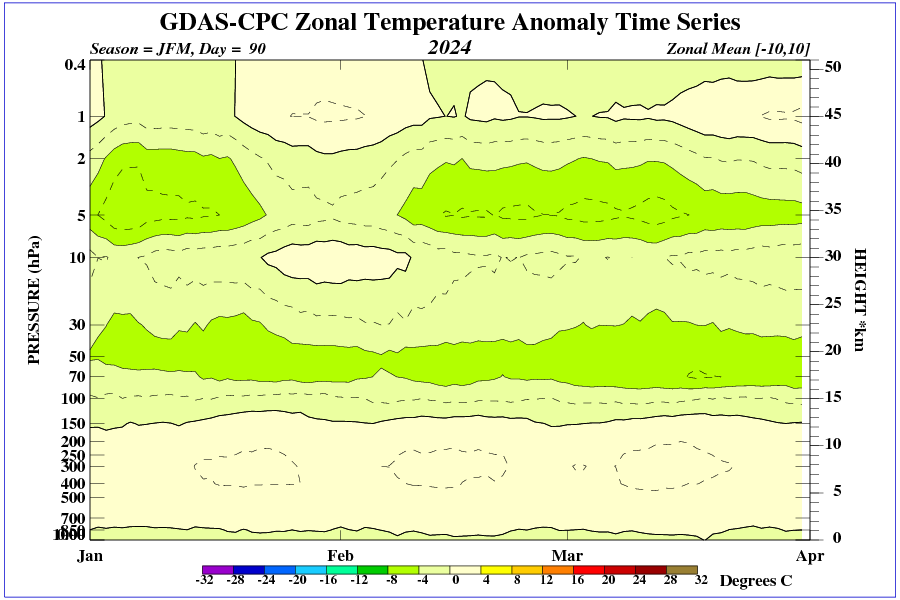
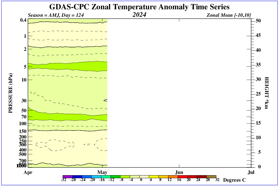
A marked decline in ozone is evident in the upper stratosphere over the southern polar circle.
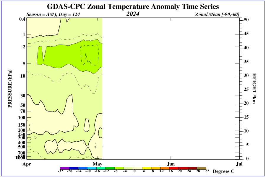
Visible low temperature in the tropics in the upper stratosphere from 25N to 25S.


A sharp drop in temperature in the lower stratosphere is seen from January to April 2024.
The temps of the globe oscillate up and down, and it now appears we are in the process of cooling, although it will take a while before all the heat put into the oceans from geothermal sources radiates out into space, hence the lag between the two.
If you ask yourself if the oceans heat the air or the air heats the ocean, maybe you can figure out it isn’t CO2 that has caused the recent warming phase. There just isn’t enough energy in the atmosphere to do it. South America just recorded it’s coldest May in 75 years and it is heading into winter. If the UAH is just 1deg C above average, the world is not in crisis.
Sunlight heats the oceans much more than the air does. Clouds cover random patches of the planet, about 65% overall….so the ocean surface temperature is controlled by cloud cover in the monthly/seasonally/annually time frame.
The mass of the oceans is about 270 that of the atmosphere plus the sea surface temperature is generally warmer than the air.
It’s specific heat capacity is about 4x that of the atmosphere so its overall capacity is about 1000x that of the atmosphere.
And yet there are still scientifically illiterate clowns that think a tiny change in atmospheric constituents causes the ocean warming.
It really is a totally DUMB anti-science little fantasy, isn’t it !
New Zealand has just had its coldest May in 15 years — NIWA