by Andy May
Introduction
In 2014, Dr. Michael Connolly and Dr. Ronan Connolly posted three important, non-peer reviewed papers on atmospheric physics on their web site. These papers can be accessed online here. The papers are difficult to understand as they cover several fields of study and are very long. But, they present new data and a novel interpretation of energy flow in the atmosphere that should be seriously considered in the climate change debate.
By studying weather balloon data around the world Connolly and Connolly show that the temperature profile of the atmosphere to the stratosphere can be completely explained using the gas laws, humidity and phase changes. The atmospheric temperature profile does not appear to be influenced, to any measurable extent, by infrared active gases like carbon dioxide.

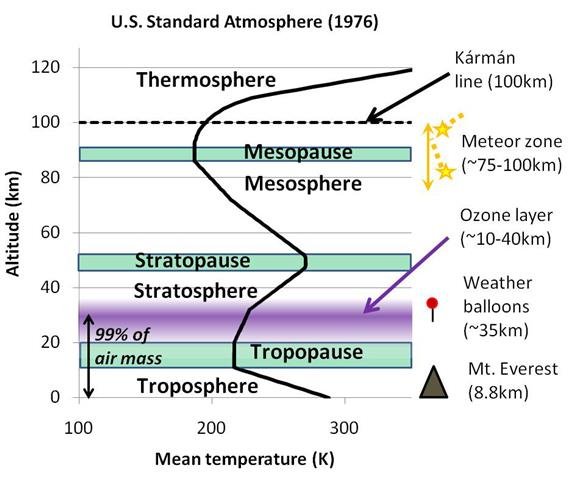
Figure 1, source Connolly and Connolly.
Figure 1 shows the “U.S. standard atmosphere.” The black curve is the standard atmospheric temperature as a function of altitude (Y axis). There are several key points that are important for this post. First, notice that the temperature decreases with altitude in the troposphere, then goes vertical in the tropopause, then it reverses course and increases in the stratosphere. Since we are discussing weather balloon data in this post, we are only concerned about the curve to about 35 kilometers. This region contains about 99% of the atmospheric mass. We will also be discussing the ozone layer, which is at the very top of our layer of investigation.
They evaluate available weather balloon data in terms of molar density and pressure. They find that, above the boundary layer (roughly the surface to 2 kilometers, the atmospheric layer that contains most of our weather), the trend of molar density and pressure is a line until the tropopause is reached. Above the tropopause it is also a line, but with a steeper slope, see figure 2. In figure 2, pressure increases to the right and altitude decreases to the right. Above the tropopause molar density decreases more rapidly with pressure, this suggests a change in the equation of state for the atmosphere above the tropopause. Region 3, the boundary layer, shows much more variability than the higher regions of the graph. This variability is due to changes in humidity and precipitation.
Multimers
A change in the equation of state in the atmosphere means that it will respond to external forces (“forcings”) differently. For the atmosphere, the equation of state is the ideal gas law, modified to account for factors that affect real gases, but not ideal gases. These include varying specific heat capacity, Van der Waals forces and compressibility effects among others. While the molar density versus pressure plots, like figure 2, strongly suggest that the equation of state has changed above the tropopause it does not tell us exactly what happened. Connolly and Connolly think that oxygen and nitrogen multimers form in and above the tropopause (see figure 3). Multimers are called trimers if they contain three molecules and tetramers if they contain four.

Figure 2, after Connolly and Connolly (2014) paper 1.

Figure 3 (source Connolly and Connolly, 2013)
This suggests that the atmosphere above the tropopause has a lower molar density, at a given pressure, than the tropospheric trend would suggest. The atmospheric composition and humidity above and below the tropopause are nearly identical, so composition is not the cause of this change.
The formation of oxygen and nitrogen multimers is a state change that can be called a phase change. If multimers form in the tropopause, they release the energy of formation to the surroundings. This may increase the temperature of the surroundings. The larger multimers have more degrees of freedom than the diatomic monomers (for example O2) and every additional degree of freedom increases the internal energy of a mole of multimers by ½RT. R is the universal gas constant and T is temperature. This is described in more detail in Connolly and Connolly, paper 2, section 2.2. In their section 2.2, the heat of formation (or enthalpy of formation) of the multimer is designated as ΔH. The molar enthalpy (H) of a gas is defined as,
H = U + PV … (1)
Where U is the internal energy of the gas, P is pressure and V is the volume.
U = ½αRT … (2)
The internal energy of the gas is equal to ½ of the degrees of freedom (α) times the gas constant (8.3145) times temperature (T). Degrees of freedom of a gas are defined here as the number of independent ways a gas can have energy. This includes translation, rotation and vibration. Internal energy is the sum of the energy in all the degrees of freedom of the gas. If ΔH is set to zero for a diatomic monomer, it is 4RT with 34 degrees of freedom (α) for a tetramer, according to table 2 from Connolly and Connolly paper 2. So, the heat of formation of a multimer can be significant and will affect the temperature of the tropopause and stratosphere. The formation of oxygen multimers probably involves the emission of microwave radiation.
In the tropopause, the lapse rate is near zero, this means, according to Connolly and Connolly, that the increase in internal energy, due to multimer conversion, is balanced with the loss of thermal energy converted to potential energy, due to gravity, at this altitude. I realize that thermal energy can be defined in different ways, but here we define it as the internal energy of the gas due to its temperature. As altitude increases and we enter the stratosphere, either more multimers are formed or they get larger and internal energy increases more rapidly than thermal energy is converted into potential energy and the air temperature begins to increase. In the troposphere, there are no multimers and thermal energy is transformed into potential energy as the altitude increases and the air temperature steadily decreases (the “lapse rate”). This causes the slope change shown for region 1 (tropopause and stratosphere), seen in figure 2.
Ozone
Ozone concentration starts to increase with altitude in the stratosphere as well. The classical explanation for the formation of ozone is called the Chapman mechanism and it is illustrated in figure 4. Chapman hypothesized that ultraviolet light (UV) striking oxygen molecules will split them into individual oxygen atoms. He then speculates, that some of these would combine with nearby oxygen molecules and form ozone.

Figure 4 (source Connolly and Connolly, 2013)
There are several problems with the Chapman mechanism. First, it requires a great deal of energy to break a diatomic oxygen molecule’s bonds. Further, if the Chapman mechanism were the only mechanism forming ozone, why would ozone concentrations, in the Northern Hemisphere, be the highest in the Arctic in the spring? The equator (the red line in figure 5) receives the most UV from the sun, yet the ozone concentration there is much less than in the Arctic, the dark blue line in figure 5. Further, one would think that the Arctic and Northern Hemisphere ozone concentration would peak in the summer, yet it peaks in the spring and falls in the summer, and begins to increase in the winter. The Chapman mechanism also has other flaws as documented here.
According to classical theory, the extra energy in the tropopause and stratosphere that reverses the negative lapse rate seen in the troposphere, comes from “ozone heating.” Ozone absorbs UV light from the sun and radiates heat which warms the tropopause and stratosphere. Yet, the tropopause stays in place during Arctic and Antarctic winters when there is no sunlight. Given these contradictions, Connolly and Connolly came up with an alternative mechanism.

Figure 5 (source Connolly and Connolly, 2014, paper 2)
Ozone formed directly from oxygen multimers also requires UV radiation, but it requires much less than is required in the Chapman process. Figure 6 shows the process described in Connolly and Connolly (2014). There a multimer of eight oxygen atoms and four oxygen molecules is transformed into two ozone molecules and one regular oxygen molecule. This process requires sunlight and abundant multimers to work, but less energy. Further, the formation of the multimers, themselves, can occur without sunlight and the formation process releases heat of formation, which helps form the tropopause and warms the stratosphere.

Figure 6 (source Connolly and Connolly, 2013)
Their idea allows ozone to form more easily and with less energy and it provides additional energy during the Arctic and Antarctic winters when there is no sunlight for months. The idea that multimers make ozone easier to form, is only one of the potential impacts of possible multimer formation in the tropopause and stratosphere. Multimer formation may also influence tropospheric weather as discussed in Connolly and Connolly paper 2.
The Weather balloon data
Weather balloons record temperature (T), pressure (P) or sometimes altitude (h), horizontal wind speed and direction, and relative humidity. Relative humidity is converted into absolute humidity using the temperature. There have been one to four launches a day from about 1,000 stations around the world – in some cases since the 1950s or earlier. That is about 13 million datasets containing data from the ground to the mid-stratosphere (~30-35km altitude). A weather balloon launch in Chile is shown in figure 7.

Figure 7 (Weather balloon launch in Chile, source: European Southern Observatory)
Nobody had analyzed the weather balloon data in terms of molar density before, but it is quite straightforward to do. Molar density, D = n/V = P/(RT) (where R=8.314, is the universal gas constant). So, all you need to do is divide the P (Pressure) values by the corresponding T values (multiplied by 8.314). The units of “D” are moles/m3.
From a climate perspective, it is better to view the molar density versus pressure plot in terms of temperature and height as in figure 8. To compute temperature, we first have to compute best fit lines to each region of figure 2 to obtain slopes and intercepts. Connolly and Connolly call the slopes “a” and the intercepts “c,” such that:
D = aP + c … (3)
Therefore, since D = P/(RT) and using the ideal gas law:
 … (4)
… (4)
“R” is still the ideal gas constant equal to 8.3145 J/(mol.K). The coefficients, “a” and “c,” are not constants and vary from place to place. Typical a and c coefficients are shown in table 1. In figure 2, the “humid” phase in table 2 is region 3, the “light” phase is region 2 and the “heavy” phase is region 1 or the tropopause and stratosphere. A spreadsheet for computing temperature from the coefficients, using equation 4, is in the supplementary materials for Connolly and Connolly, paper 1. In table 1, there are two entries for the near Artic Norman Wells site. One is for the ground (g) and other is for the tropopause/stratosphere (u). Near the poles the heavy phase (multimer formation) can occur near the ground.

Table 1, from Connolly and Connolly, paper 1.
Using equation 4 and the coefficients of the best fit lines, like those in table 1, we can estimate temperature (T). This has been done in figure 8. Most of the balloon launch sites can be fit with two or three best fit lines. In figure 8, both are fit with three lines. Lake Charles, Louisiana is sub-tropical and the boundary layer requires a separate fit due to high humidity. Norman Wells, Northwest Territories, Canada requires three because the boundary layer, in winter time, can show a phase change very like the phase change observed in the tropopause. This might be due to the formation of multimers at the surface.

Figure 8, after Connolly and Connolly, paper 1
The boundary layer is defined, in the papers, as where the absolute humidity is greater than one gram of water per kg of air. This is roughly greater than 0.1%. As figure 2 shows, the slope is relatively more variable in this region (region 3). Changes in temperature, humidity and precipitation affect the slope in this region. The boundary layer may not exist in the Arctic and Antarctic in winter, where surface humidity can be very close to zero in cold weather. Yet, slope anomalies exist there as well, sometimes going the other way as seen in the Arctic (figure 8B). These Arctic and Antarctic winter anomalies look suspiciously like the tropopause anomalies.
Connolly and Connolly found that there is a change of state, that might be a phase change, at the top of the troposphere and a similar change occasionally at the surface, in the polar regions, in the winter. After accounting for this apparent phase change, they could describe the atmospheric temperature profiles of all ~13 million weather balloons entirely in terms of the thermodynamic properties of the bulk gases and humidity. For the Earth’s atmosphere, the bulk gases are N2, O2, argon and sometimes H2O. By “thermodynamic properties”, they mean the gas laws, the role of gravity, changes in state (i.e., phase changes), differing heat capacities, etc. Of the four bulk gases, only H2O is infrared-active and the influence H2O has on the atmospheric temperature profile has nothing to do with its infrared activity. Instead, it is related to its phase changes and the fact that it has a higher heat capacity than the other bulk gases.
The temperature fits did not require consideration of the CO2 concentration or any of the other infrared-active (“IR-active”) gases. If the effect of CO2 and other greenhouse gases were as strong as predicted by the climate models, one could reasonably expect that they would affect these temperature profiles.
Most versions of “the greenhouse effect” theory argue that the infrared activity of greenhouse gases (“GHG”) alters the atmospheric temperature profile. In particular, the models suggest that as carbon dioxide is added to the troposphere by man’s emissions, the troposphere should warm. This is supposed to be counteracted by increasing the speed of cooling. Thus, they predict that the troposphere warms and the stratosphere cools due to man’s carbon dioxide emissions changing the atmospheric temperature profile. Therefore, a debate exists over whether there is a “tropospheric hotspot” signature from GHG warming. Some also argue that there must be “stratospheric cooling.” But, the key to these theories is that the IR activity of the GHGs is supposed to in some way alter at least some part of the atmospheric temperature profile. This IR-based effect is the greenhouse effect. But, if the IR activity of the GHGs doesn’t influence atmospheric temperatures, as the Connolly’s found, then there isn’t a greenhouse gas greenhouse effect!
As mentioned above, their analysis of molar density versus pressure reveals a change in slope, probably due to a phase change, that occurs above the troposphere. This phase change can explain most, if not all, of the changes in temperature behavior associated with the tropopause and stratosphere. The tropopause and stratosphere are treated as distinct regions from the troposphere because they have different temperature behaviors than the troposphere. That is, the lapse rate approaches zero in the tropopause and becomes positive in the stratosphere. While this is true, the tropopause and stratosphere share the same molar density vs. pressure slope, intercept, and equation of state.
Multimers and the Ozone Layer
In Connolly and Connolly’s paper 2, they argue that the phase change identified in their paper 1 is due to the formation of oxygen (and possibly nitrogen) multimers, i.e., (O2)n, where n>1. The formation of multimers in the atmosphere is not a new idea and has been studied by Slanina, et al., 2001.
They also noted that if multimers are forming in the tropopause and the stratosphere, there is an alternative mechanism for the formation of ozone, which is much more rapid than the standard Chapman mechanism. That is, ozone (O3) could form directly from the photolysis of oxygen multimers, for example, a trimer (three linked O2 molecules) of oxygen could dissociate into two ozone molecules: (O2)3 + uv light → 2O3.
There is a remarkable correlation between the proposed phase change conditions and ozone concentrations, see figure 9. This is consistent with the Connolly’s mechanism for the formation of ozone, and suggests that the ozone is generated rapidly in situ. Table 2 lists the computed phase change conditions for 12 different regions, separated by latitude, around the world:

Table 2, Source: Connolly and Connolly paper 2

Figure 9, Source: Connolly and Connolly paper 2
Figure 9 shows the monthly variation of the optimal phase change pressure for several of the regions versus ozone formation (from NASA’s Total Ozone Mapping Spectrometer) for the same region. The correspondence between them is clear. It is interesting that the optimal pressure conditions for the phase change vary dramatically from month to month in each latitude band in figure 9 and that the level of ozone also varies dramatically from month to month. This suggests that ozone creation is very fast in the upper atmosphere, something that is consistent with the Connolly’s hypothesis, but not consistent with Chapman’s. It is also not consistent with the hypothesis that chlorofluorocarbons destroy the ozone layer, but that is another story.
Local Thermodynamic Equilibrium
Connolly and Connolly have shown, using the weather balloon data, that the atmosphere from the surface to the lower stratosphere, is in thermodynamic equilibrium. They detected no influence on the temperature profile from infrared active (IR-active) gases, including carbon dioxide. This is at odds with current climate models that assume that the atmosphere is only in local thermodynamic equilibrium as discussed by Pierrehumbert 2011 and others.
Climate models split the atmosphere vertically into many different layers, each a few kilometers thick, then the layers are broken up geographically into grid boxes. Each grid box is assumed to be in local thermodynamic equilibrium (LTE). These boxes are assumed to be thermodynamically isolated. However, within each grid box, the total energy content is assumed to be completely mixed. Because each box is isolated from the surrounding boxes, the rates of IR emission and absorption from the box are a function of:
-
The IR flux passing vertically through the box
- The current average temperature of the box
-
The concentrations of each of the IR-active gases in the box
Since they are thermodynamically isolated from each other, if a grid box absorbs more (or less) IR radiation than it emits, this will alter the energy content and average temperature of the box. For this reason, a grid box can develop an energetic imbalance relative to the surrounding grid boxes through radiative processes. Therefore, in the models, the presence of “greenhouse gases” (e.g., CO2) alters the underlying atmospheric temperature profiles. But, is this LTE assumption valid? So far, it has simply been assumed to be the case.
What would happen if the grid boxes are not thermodynamically isolated? Well, if one grid box becomes “hotter” or “colder” due to radiative heating/cooling than the surrounding boxes, then energy would flow between the neighboring grid boxes until thermodynamic equilibrium was restored. If the rates of energy flow are fast enough to maintain thermodynamic equilibrium then the radiatively-induced imbalances from the IR-active gases would disappear. Instead, the atmospheric temperature profile would be determined by the thermodynamic properties of the bulk gases. This is what Connolly and Connolly found was happening.
With thermodynamic equilibrium, we would still expect to see, the often observed, up-welling and down-welling IR radiation. We would also still expect the total outgoing IR radiation to remain roughly in balance with absorbed incoming solar radiation, as we currently observe. And, we would expect the IR spectrum to show the peaks and troughs characteristic of the main IR-active gases, i.e., H2O, CO2 and O3. However, Connolly and Connolly found that the IR-activity of these gases does not alter the atmospheric temperature profile.
Pervection
The standard mechanisms for energy transmission within the atmosphere usually considered are radiation, convection (of which there are three types: kinetic, thermal and latent) and conduction. Because air is a poor heat conductor, conduction’s role in atmospheric energy transmission is negligible. That initially would appear to leave just radiation and convection. Both radiation and convection move thermal energy slowly, too slowly to keep the atmosphere in thermodynamic equilibrium. However, we know from thermodynamics that thermal energy can be converted to work and transmitted and then turned back into thermal energy. Thermal energy transfer is not the only method of energy transfer at work in this equilibrium process.
Connolly and Connolly found that there is almost no experimental data on the rates of vertical convection outside of clouds and above the boundary layer. But, from the limited data they have, the rates of vertical convection appear to be too slow to maintain thermodynamic equilibrium from the surface to the stratosphere.
They found an additional energy transmission mechanism which seems to have been neglected, “through-mass” mechanical energy transmission. Unlike convection where the energy is only transported by a moving air mass, this mechanism allows mechanical energy to be transmitted through the air mass without the air itself having to move significantly. This is like conduction, except that conduction involves the transmission of thermal energy, while this mechanism involves the transmission of mechanical energy. To distinguish it from “convection” (which comes from the Latin for “carried with”), they use the term “pervection” (from the Latin for “carried through”). In this process, molecules collide transmitting mechanical energy to one another. An analogy would be a long tube filled with ping-pong balls and the tube is only wide enough for one ball. If a ping-pong ball is forced in one end of the tube, one will immediately be forced out the other end. None of the ping-pong balls move very far, but the energy is quickly transmitted, mechanically, a long distance.
In Connolly and Connolly paper 3, they designed a series of controlled experiments to try to quantify the relative rates of energy transmission of each of these mechanisms in air. Their experiments showed that, at ground level, energy transmission by pervection (aka “work”) is several orders of magnitude faster than conduction, convection or radiation! This then explains why the troposphere and stratosphere are not thermodynamically isolated, as the climate models assume.
Pervection is a mechanical energy transmission mechanism, not a thermal energy transmission mechanism, in common thermodynamic terms it can be considered “work.” Mechanical and thermal energy can be converted to one another as thermodynamics teaches us. So, either energy transmission mechanism can, and will, act to restore thermodynamic equilibrium. This also highlights why it is important to consider multiple types of energy and energy transmission mechanisms.
Conclusions
The three papers by Connolly and Connolly provide new data and analysis that show the IR-active trace gases in the atmosphere have an insignificant effect on the atmosphere’s vertical temperature profile. They show the atmosphere, at least to the lower stratosphere, is in thermodynamic equilibrium which invalidates the local thermodynamic equilibrium assumption used by the global climate models.
Unlike other critiques (Jelbring, 2003, Johnson 2010, O’Sullivan, et al. 2010, Hertzberg, et al. 2017, and Nikolov and Zeller, 2011) of the carbon dioxide climate control knob hypothesis (Lacis, et al., 2010), this analysis explains two lines of evidence often used to justify the carbon dioxide greenhouse effect:
-
Why is the lapse rate positive (temperature increasing with height) in the stratosphere?
- Why do we observe both upward and downward traveling IR radiation in the atmosphere?
The lapse rate, which averages about -6.5°C per kilometer in the troposphere, goes vertical and eventually reverses sign in the tropopause and stratosphere due, at least in part, to the formation of multimers according to Connolly and Connolly. The formation of multimers releases energy, which can account for at least some of the tropopause and stratospheric heating. IR-active atmospheric gases like water vapor and carbon dioxide do radiate IR in all directions and this can be detected, it is just that this radiation does not affect the atmospheric temperature profile significantly according to Connolly and Connolly’s work.
It takes less energy to form ozone directly from oxygen multimers than from splitting diatomic oxygen molecules, although both require UV light. Further, ozone formation does correlate well with the conditions required for multimer formation. Multimer formation does not require sunlight and can occur at night. Also, ozone concentrations in the ozone layer vary rapidly, suggesting ozone is created and destroyed monthly. This is inconsistent with the Chapman process.
The key problem with the conventional idea of IR-active gases, like carbon dioxide, influencing atmospheric temperatures is the concept that the atmosphere is only in local thermodynamic equilibrium. The weather balloon data strongly suggest that the atmosphere is in thermodynamic equilibrium, meaning IR-active gases have little to no influence on atmospheric temperatures. For this to be true a very fast energy transfer mechanism must be at work. Connolly and Connolly suggest that this transfer mechanism is mechanical in nature. Using thermodynamic terminology, the mechanism is “work.” They have proposed a name for the mechanism and call it “pervection.”
Currently, the multimer formation in the tropopause and stratosphere is speculative and requires experimental verification. Likewise, the details of forming ozone from oxygen multimers need to be worked out and documented. Pervection is a proposed name for a relatively obvious form of energy transfer that we observe all the time and has just been overlooked for some reason in climate science. Air is compressible, of course, but it does transmit mechanical energy. BB guns, air compressors and inflatable tires wouldn’t work without this energy transfer process.
So, clearly the Connolly and Connolly ideas need further work, but they have put together a very coherent and detailed hypothesis that deserves serious consideration. It is, at least, as well documented and supported as the conventional carbon dioxide greenhouse theory.
For those that want to read a more detailed summary of the Connolly’s work that includes a description of their laboratory work, I refer them to the Connolly’s summary here and to their three papers, linked at the top of this post.
A very good article, Andy, that makes accessible the Connolly’s views on the atmosphere.
Their work sounds plausible to somebody as ignorant as myself on these issues, but what really should matter is what the experts think of their proposals. As far as I can tell their work does not contain experiments, but a reinterpretation of the evidence. If they can demonstrate that their reinterpretation is better at explaining the observations, they should not have much problem in getting it published.
However it bothers me that they need a new term to define a vertical transfer of energy in the atmosphere. Scientists have been studying that subject since the dawn of modern science. We are now living in a time with the highest proportion of scientists in society and the highest number by far, and they work in a very competitive environment. They are very intelligent people always on the look for new important discoveries in their areas of study. It is therefore harder than ever for non scientists to make important contributions to science. Not impossible, but not easy at all.
I don’t know, but their pervection sounds quite a lot as the vertical gravity waves that transfer momentum and energy from the surface and troposphere upwards. Scientists have been studying them for the past 50 years and have a good understanding of their physics.
My take on pervection would be the classic Mexican Wave or watching cars/traffic at sets of traffic lights.
So, all is calm in a group of molecules (all at the same temp) then one of them (possibly a CO2 molecule) catches a passing package of energy (photon)
It then, almost instantly ‘jumps’ – it becomes excited or more energetic than its immediate neighbours and gives one of them an almighty jolt.
In turn it ‘jumps’, bumps its neighbour who then bumps the next then the next.
Just like at the traffic lights, each car, in turn, waits for the one in front of it to start moving before it does. Or the Mexican Wave.
Or ripples on a pond when a pebble is thrown in.
And the pebbles come from, or are, packets of energy ‘captured/trapped by ‘green house gases’
More you think about it, it is sound propagation.
Is it directional?
IOW, would/does/do sound waves preferentially accelerate into lower pressure or lower temperature. i.e. go down or up with any preference.
Or sideways by preference which is why climate models can’t/don’t handle them
If this wave formation with vertical energy transport is still further thought, then the mere upward transport of air with convection as a secondary effect can trigger such a transfer of energy from molecule to molecule. Even after the earthquake in Nepal in 2015, it was proved that the ozone layer has been reacting to the earthquake in an incredibly short time (21 minutes). The question now arises, why did he react. Because of electromagnetic waves, which were triggered by the quake or by the displacement of air masses (also air masses have a mass) by the quake and passing of the kinetic energy from molecule to molecule up into the ozone layer.
“As far as I can tell their work does not contain experiments, but a reinterpretation of the evidence.”
It seems to me an obvious experiment would be to detect these trimers and tetramers in gas samples at realistic atmospheric conditions. This should not be too hard to do.
They say there is a phase change. That could be experimentally checked.
Javier, they have experimentally verified the speed of pervection. They have also shown that the lower atmosphere is in thermodynamic equilibrium. The multimer formation is educated speculation, so is the ozone formation mechanism that they propose.
So why do you and the authors prefer this new multimer based explanation as against the ozone formation mechanism which has been demonstrated convincingly for decades via observation ?
Do you have references to ozone formation from lab results using the UV proposed mechanism? The experimental test of such a mechanism should be straightforward at the pressures indicated. The vibrational excitation of the resulting ozone should be measurable.
“The atmospheric temperature profile does not appear to be influenced, to any measurable extent, by infrared active gases like carbon dioxide”
The lapse rate feedback in AGW is small and very difficult to measure given errors in the observation systems
The change in the vertical temperature profile takes a very long time to develop.
Sorry skeptards
http://geotest.tamu.edu/userfiles/216/dessler09.pdf
This appears one of the problems that besets so much of climate science.
It is just like Climate Sensitivity (if any at all) to CO2. The signal is just too difficult to measure, since if there is any signal it has yet to raise its ugly head over and above the noise of natural variability in temperature, notwithstanding the use of our best and most sensitive measurement devices, and the inherent error bounds of the equipment and practices used.
Perhaps one day we will be able to detect it, should it exist.
Steven, bad link at least here…
The details are sooo HARD! It’s sooo much easier to declare the science settled and collect a cheque sitting in front of a computer changing all the input parameters except CO2 effect and feedback signs. If we solved this thing we’d have to get real jobs!
it’s not even hard to find if you look.
It was clear and calm all night.
Steven Mosher, if the effect is that small, then AGW really has little to support it. Which is exactly the point the Connolly’s are making. Interesting point of agreement, I would not have expected you to say that.
Your link is bad Steven, but I’ve seen other articles that also admit that the effect of AGW on the vertical temperature profile is very small. You and the Connolly’s are not the only ones. However, what it means is that AGW is not significant – that point is often lost. If the atmosphere is in thermodynamic equilibrium to 35 km, the whole AGW argument falls apart.
Andy,
Not only is his link bad, so is his attitude. Using “skeptard” is insulting and I certainly think even less of him for it. It belies an arrogance that reflects on his lack of humility.
Very interesting Andy. This is a good example why gatekeeping and settled science propaganda is certain to lead away from good science. I’m with Steve McIntyre on his appraisal of most of the CliSci Team =>
They would be high school science teachers in an earlier generation if they were lucky.
Can multimers be sampled and maybe kept at their ambient pressure and temperature ? Can one take a sample of air in the laboratory and reduce its temperature and pressure to that above the troposphere and make these molecules?
I’m not clear how polymerizing oxygen would alter the density of the air. It has to mean that there are more oxygen atomic units per cubic meter and it still acts like an ideal gas. If the oxy ‘mers’ were stronger oxydizers, they may also react with nitrogen. That would increase the density of the air also, and NO2 is only 4% lighter than a trimer of oxygen. Who knows what the effect on chemistry of upper layers that ultraviolet, cosmic rays, ozone, etc etc have.
The multimers are speculation by the Connolly’s at this point. We are hoping that the lab work will be done at some point.
See this comment for some of what you are asking: https://wattsupwiththat.com/2017/08/22/review-and-summary-of-three-important-atmospheric-physics-papers/comment-page-1/#comment-2587932
The only gasses that form dimers at low pressure and temperature are the organic acids, like acetic acid (the acid in vinegar), and HF which likes to form a cyclic hexamer at least. These molecules do this due to their extreme hydrogen bonding potential. Water, surprisingly, does not form a dimer to an appreciable extent at low pressure, even though it is the king of hydrogen bonding. as my previous comment (yet to be posted, hint hint…) said, the authors need to explain why this multimer formation happens when no one else has measured it.
Well, I started reading the paper, but got stuck early on. It seems that the data they are actually working from is measured pressure and temperature. So they define molar density D = P/RT; the identification of that as density comes from the ideal gas law (which is ideal…).
So then, in Figs 4/5, they plot D against P. Is the slope of this not just 1/RT? And the “regime changes” just changes in T?
Nick, you are not clear. Are you saying that the paper has fundamental problems right at the beginning? I focused on the requirement for a substantial proportion of the atmosphere to exist as “multimers” which seems at first glance to be unlikely, given the energy of the system and the weakness of van der Waal’s forces.
seaice
“Are you saying that the paper has fundamental problems right at the beginning?”
Yes. There’s just no information there. They have readings of P and T. Using the IGL, you can then calculate density. That’s it. You can’t use the calculated density to tell you more about temperature. Or deviations fro IGL, that might lead to multimers or something. For that you need independent data on density, or some such. This stuff is circular.
I tend to agree with you almost. Is it not the rate of change in temperature.?
Nick, the answer you seek is too much for a comment. Read section 3.2 in paper 1. Especially lines 396 to 404. Check figure 8 and the spreadsheet in the supplementary materials. I think that will make it all clear to you.
Andy,
I read it (3.2), but it’s even weirder. We start with measured P and T. Then they fit a line to D=P/RT vs P, and then deduce T from the slope of the line. WUWT?. T was the starting information. Maybe this gives a kind of smoothed version, but it’s very roundabout.
Nick, I’m not going to disagree with your maths analysis, I think you are correct. But, I think what the Connolly’s are getting at is that the change in slope at the tropopause suggests a change in the equation of state. The change in temperature gradient also suggests the same thing, but is harder to interpret. The second unusual aspect of the graphs is that the same line works in the stratosphere, temperature plots make it look like the stratosphere is different. I don’t know what causes the equation of state to change, neither do the Connolly’s, but they came up with a falsifiable hypothesis to explain it. If the lab work is done. maybe we will learn something. I will leave it here and, hopefully, the Connolly’s will chip in.
Nick, One other point. The change in temperature gradient at the tropopause is the question here. If 1/T is the slope, we still have the question of why the temperature gradient changes, right? The temp gradient changes again in the stratosphere, why does the molar density gradient not change there?
Andy,
“The change in temperature gradient also suggests the same thing, but is harder to interpret.”
They aren’t adding anything by this device of doing a bit of algebra so that 1/T turns up at the slope of another curve, so they talk about that instead. The change in temperature gradient at the tropopause has been known for a very long time, and has a standard interpretation that few seem to find even problematic, let alone requiring the postulation of otherwise unknown molecular behaviour.
Andy and Nick: The problem with this “paper” is fairly easy to spot. Equation 8 of Paper 1 is clearly wrong. I says that atmospheric temperature is a function of P and a bunch of constants. So is equation 7, which says that pressure is a simple function of temperature and some constants.
The pressure at any altitude is simply the weight of the air above that altitude. It is not a function of temperature. What Connelly is forgetting is that the VOLUME of air at any location expands of contracts to satisfy the ideal gas law GIVEN the local temperature and pressure. And volume, of course, effects density.
Consult the WIkipedia article on “Scale Height” of the atmosphere. It derives:
dP/P = -dz/H where H = kT/Mg
P = P_0 * exp(-z/H)
For modest changes in z (compared with H), the first two terms of the Taylor expansion give P = P_0*(1 – z/H). H ranges from 8500 m at 290 K to 6000 m at 210 K
In the troposphere, there is a fairly linear relationship temperature and altitude – the lapse rate and an approximately linear relationship of modest changes in altitude between pressure and altitudeIn an isothermal atmosphere he relationship between pressure and altitude. In that domain, Connelly’s D = aP + c can be adjusted to fit radiosonde data. Once one leaves regions where there isn’t a constant lapse rate, this relationship breaks down – as it should. There is NO linear relationship between D and P – there only appears to be in regions with a constant lapse rate and modest changes in altitude compared with H . (The next term in the Taylor expansion is +(z/H)^2/2. At low altitudes where there is a thermal inversion, there are problems.
I don’t claim to have thoroughly read and understood the 30 pages of Paper 1. I presume that derivations in the appendix always are always making an unwarranted assumption: that T is constant and V is a function of P. That V is constant so that T is a function of P. Or that change are adiabatic, so that total energy is conserved with altitude.
Frank and Nick, I think both of you are completely missing the point. See Ronan’s explanation here. He tackles it from a slightly different viewpoint. Their work is very significant and important, but a bit hard to understand. I think if you spend a little more time with their papers you will get it. https://wattsupwiththat.com/2017/08/22/review-and-summary-of-three-important-atmospheric-physics-papers/comment-page-1/#comment-2589151
Frank, Equations 7&8 describe an atmosphere in thermodynamic equilibrium. They are not wrong or right necessarily, simply descriptive. If they hold and match measurements, the atmosphere is in thermodynamic equilibrium. 13 million weather balloons, launched over 50 years, say they describe the atmosphere. You make an assumption, without any evidence to support it, that they can’t be correct. If you can find data that supports your assertions, I’ll listen. I doubt there is any however.
The light phase? That’s the vapor phase in a heat pipe
Like this
https://en.wikipedia.org/wiki/Heat_pipe#Variable_Conductance_Heat_Pipes_.28VCHPs.29
“Norman Wells, Northwest Territories, Canada requires three [separate fits] because the boundary layer, in winter time, can show a phase change very like the phase change observed in the tropopause. This might be due to the formation of multimers at the surface.”
The inversion layer is now caused by *the formation of multimers*, instead of that massive heat sink called *the ground*.
It could be an inversion, I don’t argue that point.
Nick, I am almost with you. Is is not a rate of change in temperature that causes the change in the regime.
Andy,
Thanks for doing this summary of our 3 “Physics of the Earth’s Atmosphere” papers! There’s a lot of material and concepts in the papers, but you’ve done a good job of summarising most of the main points.
Unfortunately, I’m quite busy this week so I might not have time to answer all the comments. But, I’ve time for a few quick responses to some of the questions above, and I’ll try to set aside more time this time tomorrow.
1) On pervection
With regards to “pervection”, for a detailed discussion see Paper 3.
But, the key point is that pervection is not the same as either convection or conduction, but it has some similarities to both.
There are several different types of convection: thermal convection (e.g., movement of hot air), latent convection (e.g., movement of water vapour) and kinetic convection (e.g., constant temperature winds). However, in all cases, energy is transported from one region to another by the physical movement of the energetic molecules. The linguistic roots of the term “convection” mean “carried with”. In what we refer to as “pervection”, the molecules themselves do not have to be physically transported for the energy to be transmitted. Instead, the energy is transmitted “through” the molecules, and the molecules remain where they were (on average). To compare and contrast this with convection, we kept the “-vection” (“carried”) suffix, but used the “per-“ (“through”) prefix instead of “con-“ (“with”).
Conduction is also a “through-mass” energy transmission mechanism. However, it involves the transmission of thermal energy, not mechanical energy.
For those who are uncomfortable using the term “pervection”, you could use the term “through-mass mechanical energy transmission” instead. That was actually our original term for it, but we felt “pervection” was more succinct.
Keith J suggested above that it is “sonic”. Sonic (or acoustic) energy transmission is indeed a form of what we refer to as “pervection”, but from our laboratory measurements we find “acoustic pervection” is at least two orders of magnitude slower than the rapid “through-mass mechanical energy transmission” we are finding.
2) On multimers
In Paper 1, we identified a previously-overlooked phase change associated with the transition between the troposphere and tropopause/stratosphere. In Paper 1, we avoided speculating on what is actually causing this phase change, and instead focused on describing the phase change itself.
In Paper 2, we offer the best explanation we have come up with so far, which is the partial multimerization of O2 (and possibly some N2), and a detailed rationale of why we came up with this theory. However, regardless of whether our multimer theory is correct, incorrect or partially correct, the phase change is remarkably clear and consistent once you start looking at the weather balloon data in terms of molar density vs. pressure.
To illustrate this phase change a bit clearer, here is a video showing the temperature vs pressure (top), molar density vs pressure (middle) and horizontal wind speed vs pressure (bottom) plots for all the weather balloons launched in 2012 from Valentia Observatory (Ireland):
Notice in the molar density (D) vs pressure plots (middle panels) how the rate of change of D with pressure is linear for the troposphere, and linear for the tropopause/stratosphere, but that the slopes of these lines are different?
This change in slope corresponds to the phase change we are referring to.
In Section 2.2 of Paper 2 we provide a detailed justification for our multimer explanation. We spent a long time considering (and discarding) multiple different theories, and that is the only one we’ve come up so far that seems to explain all the data. If anyone has a better explanation for the phase change which also resolves the issues we raised in Section 2.2, we’re open to suggestions. But, if you haven’t read that section yet, I’d recommend reading it first.
Unfortunately, I have to leave now. So, sorry if I haven’t gotten around to addressing all of your comments. But, I will try and get back for more tomorrow.
Mods
This ought to be elevated to the top of the post as it gives further understanding of some of the important concepts involved.
Richard, I put a link near the top.
Thanks very much Ronan, this helps a lot. Looking forward to additional comments. Thanks for taking the time, I know you and your father are very busy.
It’s because the temperature gradient changes !
You are plotting D= P/RT against P therefore a plot of P against P will give a straight line. With a decreasing temperature then you put a bias on one of the P the one you call Density . By increasing temperature you start reversing the bias and there is a change in direction of the graph, there is no new phase! Gas is a gas they are always miscibile all gases are a single phase. Now you speculate on a multi met. But they form with increasing pre sure not decreasing. Send your paper for peer review and you will get the same comments.
No multimers, no second phase in a gas. Gas is a gas. It does not form 2 phases. Liquids can gases by definition do not.
The Connellys are not talking about phase change nor about chemical enthalpy change (like that of oxygen to ozone) but dimerization (or more) of gases to explain the gross deviation of the Ideal Gas Law. IGL deviations are expected at high pressures and low temperatures (compared to standard temperature and pressure).
Water vapor is a gas. It has limited miscibility in air. Somehow it makes its way past the stratopause to form noctilucent clouds in the mesosphere if only in hemispherical summer. This implies mesosphere lapse rate changes with season…why?
Dave, the slope of the line should be 1/T. Why are there 2 slopes? Why is the tropopause slope the same as the stratosphere slope? The formation of multimers is one possible hypothesis, do you have another? I agree multimers, under these conditions, are speculative. Perhaps “phase change” is an inappropriate phrase. But, certainly the equation of state has changed, no doubt about that. The lines, showing a linear relationship between D and P also show no deviation from equilibrium which we should see if greenhouse gases are having an effect.
Between the 1950’s and 1976 NASA (and it’s predecessor the National Advisory Committee for Aeronautics – NACA) were responsible for establishing the properties of the atmosphere to support US military, rocketry and later the space programs.
They developed a model of the atmosphere that was consistent with literally millions of data points from measurements on the ground, from aircraft, and high-altitude research balloons. The final model, published in 1976, is called variously the NASA standard Atmosphere and the US Standard Atmosphere. It is essentially identical to the ISO standard atmosphere.
The model was based on physics and thermodynamics, and is essentially independent of the chemical composition of the atmosphere.
The most important equation for the troposphere, which includes nearly 95% of the air, is the equation for the Adiabatic Lapse Rate, dT/dh = -g/Cp. This describes how the temperature T of the atmosphere varies with height h above the ground because of the acceleration of gravity g and the heat capacity of the air at constant pressure Cp.
For the earth Cp is slightly a function of the heat capacities of the separate components of the air, but the heat capacity of carbon dioxide is nearly the same as those of nitrogen and oxygen. The concentration of carbon dioxide has a negligible influence on the heat capacity of air as a whole.
The only gas that can significantly change the heat capacity of air, depending on its concentration, is water vapor. The adiabatic lapse rate for dry air is a decrease of 9.8 °C/km (5.38 °F per 1,000 ft) (3.0 °C/1,000 ft). The moist adiabatic lapse rate varies strongly with temperature. A typical value is around 5 °C/km, (9 °F/km, 2.7 °F/1,000 ft, 1.5 °C/1,000 ft).
As one’s altitude increases the temperature decreases at this rate. Conversely, as one’s altitude DECREASES, temperature INCREASES accordingly.
The reason the atmosphere of Venus is so much warmer than that of earth is not its CO2 concentration but its mass. The atmosphere of Venus weighs about 92 times as much as that of earth, so pressures are correspondingly higher, and the atmosphere is correspondingly thicker. At an altitude on Venus where the pressure is about the same as that of Earth’s atmosphere at sea level, about 50 kilometers(!), the temperature is about 55°C (328°K versus Earth’s average 288°K). Given that the earth is 38% farther from the sun, and correspondingly the sunlight on earth is weaker, this is not unexpected from simple solar irradiance calculations.
The mythical ‘runaway greenhouse effect’ on Venus is simply a political fiction grown from a pedagogical shortcut created no doubt, to avoid trying to explain the ‘adiabatic lapse rate’ to scientifically untrained minds.
If there is a radiant GHE on Venus, it does not work in the same way as the postulated theory for the radiant GHE on Earth.
At the heart of the radiant GHE theory is that Earth’s atmosphere is largely transparent to the wavelength of incoming solar irradiance but somewhat opaque to the wavelength of outgoing/upwelling LWIR.
Now Venus is very different in that the Venusian atmosphere is almost completely opaque to the wavelength of incoming solar irradiance. The Russian Venera Mission measured solar irradiance received at the surface of Venus at just 17W/m2.
Venus also has sulfuric acid virga. No free water as there is considerable sulfur trioxide gas. This is sulfuric acid anhydride. So it could be said there is oleum controlling the climate of Venus . Compare the physical properties of oleum to water.
tadchem August 22, 2017 at 12:58 pm
The ALR does not describe how the temperature of the atmosphere varies with height, but how the temperature of a RISING or SINKING parcel of air varies with height, assuming the atmosphere surrounding the parcel is in hydrostatic equilibrium and that no heat exchange takes place with the surrounding atmosphere.
“The atmospheric temperature profile does not appear to be influenced, to any measurable extent, by infrared active gases like carbon dioxide.”
So are people going to stop den*ing this now? This has been accurately shown in mathematical models for years. Another paper further detailing this was just published recently.
https://www.omicsonline.org/open-access/New-Insights-on-the-Physical-Nature-of-the-Atmospheric-Greenhouse-Effect-Deduced-from-an-Empirical-Planetary-Temperature-Model.pdf
This has been dealt with in previous posts. Nikolov (or Volokin) are basically doing a curve fitting exercise.
Yes, their work is essentially worthless, and that’s not just my opinion.
I would not be so quick to dismiss out of hand the point being made in that paper.
One reason for which is Mars, and what NASA says about terraforming.
It is generally accepted that despite Mars having some 959,700 ppm of CO2, which, on a physical numerical basis, is an order of magnitude more CO2 molecules than exists in Earth’s atmosphere, Mars has no GHE. The reason put forward is that the Martian atmosphere is not sufficiently dense/it lacks pressure.
Now that reason (ie., the lack of density/pressure of the atmosphere) is coming close to saying that what keeps a planet warm is not molecules of GHGs, but rather the presence of a thick and dense atmosphere.
NASA’s proposal for terraforming is to increase the density of the atmosphere and hence the pressure, not to increase CO2 from 959,700 ppm to say 970,000 ppm. Indeed, NASA wants to create a breathable atmosphere which inevitably means that the concentration of CO2 must be reduced down from 959,700 ppm.
There is yet a lot to learnt and understood.
Ronan said:
“the molecules themselves do not have to be physically transported for the energy to be transmitted. Instead, the energy is transmitted “through” the molecules, and the molecules remain where they were (on average).”
Well you can say that for an atmosphere in hydrostatic equilibrium the molecules all stay in the same place ON AVERAGE but that doesn’t mean much. At best it just means that the atmosphere as a whole remains suspended off the surface indefinitely.
Within the body of an atmosphere there is as much movement up as there is movement down on average so that the whole atmosphere is constantly in motion.
The amount of Potential Energy (PE) required to raise half the bulk of the atmosphere upwards against gravity is huge and the amount of Kinetic Energy (KE) released when half the bulk atmosphere descends with gravity is likewise huge.
Anyone who thinks that those two energy transformation processes are not enough to drive observed atmospheric behaviour are simply wrong.
Energy is not transmitted through stationary molecules. Energy is transformed from heat to form potential energy in uplift and from potential energy to heat in descent.
Our entire global air circulation including the weather systems and climate zones within the troposphere and the Brewer Dobson circulation in the stratosphere are driven by the constantly varying balance of kinetic and potential energies at any given point in three dimensions within the atmosphere.
People should read up on Convectively Available Potential Energy (CAPE in meteorology) and think it through.
Ronan said:
“In Section 2.2 of Paper 2 we provide a detailed justification for our multimer explanation. We spent a long time considering (and discarding) multiple different theories, and that is the only one we’ve come up so far that seems to explain all the data. If anyone has a better explanation for the phase change which also resolves the issues we raised in Section 2.2, ”
The historical understanding is that it is the presence of ozone in the stratosphere that reacts directly with incoming solar radiation so as to heat up and reverse the lapse rate slope.
That being the case could Ronan please paraphrase briefly why he needs to invoke phase changes and multimers for those of us who may not have time to read all his papers.
Stephen, phase changes and multimers were chosen as the most likely explanation that fit all of the data. Experimental verification is still needed. But, the idea fits what we know, alternative explanations are requested if you have one. Experimental data is very welcome.
What we do know, is the atmosphere is in thermodynamic equilibrium to 35 km (99% of the atmospheric mass) and energy transmission is fast enough to maintain equilibrium. These facts alone invalidate AGW. The only way AGW can work is if thermal energy can build up at the surface, that is be delayed on its trip to outer space, due to greenhouse gases like CO2. For the AGW hypothesis to be viable, the vertical temperature profile of the atmosphere has to change. If the atmosphere is in equilibrium, AGW is bovine excrement. Sorry, but that is the way it is.
In what way does ozone creation in the lower stratosphere fail to fit all the data?
As regards AGW I agree with you but the answer is readily available in the broader science without invoking ‘pervection’ or ‘multimers’.
Red oxygen, the multimer they talk of has been characterised at 100 000 atm pressure in solid oxygen. It cannot exist as a gas, if this is their most l ikeley explanation it does not bode well for the rest of their conclusions.
I have pondered the same conundrum. If AGW is defensible, trtropospheric lapse rate should change with increasing carbon dioxide. Because carbon dioxide adds to atmospheric mass and density and because the bulk of convection is water vapor, negative feedbacks cancel any hypothetical forcing.
A plot of density agaist pressure is a plot of pressure divided by temperature against pressure.
Whilst the temperature is decreasing with pressure a bias will be put on the slope of pressure vs pressure. We then start increasing the temperature with pressure , then the slope of pressure/temperature vs pressure wil now change its slope. There that is a much simpler and better explanation than invoicing a second gas phase!
Molar density Dave, not density. Let’s be clear what we are talking about.
Molar density is proportional to density. The kink in the graph will be exactly in the same position i.e. that where the temperature gradient changes, also please see my post on red oxygen. T etramers only exist at 100 000 atmospheres pressure and oxygen is solid
Dave, see my answer to Nick on the same subject. Here:
https://wattsupwiththat.com/2017/08/22/review-and-summary-of-three-important-atmospheric-physics-papers/comment-page-1/#comment-2588435
“Nick, I’m not going to disagree with your maths analysis, I think you are correct. But, I think what the Connolly’s are getting at is that the change in slope at the tropopause suggests a change in the equation of state. The change in temperature gradient also suggests the same thing, but is harder to interpret. The second unusual aspect of the graphs is that the same line works in the stratosphere, temperature plots make it look like the stratosphere is different. I don’t know what causes the equation of state to change, neither do the Connolly’s, but they came up with a falsifiable hypothesis to explain it. If the lab work is done. maybe we will learn something. I will leave it here and, hopefully, the Connolly’s will chip in.”
The same information is in temperature, but that begs the question, why the change in temperature gradient?
The temperature gradient changes at the tropopause because of ozone creation when sunlight acts on oxygen at that height and above. At lower levels in the tropopause the primary heating process for our largely non radiative atmosphere is conduction from the heated surface at the base.
Once one reaches the tropopause, radiative effects involving ozone start to take over. The lower atmospheric density above the tropopause provides less of a shielding effect for the oxygen molecules and so ozone forms more readily and takes over from the effect of conduction at the surface.
What are the effects of H2O vapor and CO2? What are the effects of increasing their concentrations?
The emission and absorption spectra of H2O vapor and CO2 are well-established from laboratory research, and the upward and downward transmission of LWIR have been measured and are reasonably concordant with Planck’s law. (distribution) and the Stefan-Boltzman law (intensity).
Is all of that irrelevant?
For those of us who aren’t chemists, what are the bonds in a multimer?
They are bonds much weaker than covalent bonds. The strongest of these are hydrogen bonds where hydrogen bridges between two atoms of oxygen or fluorine, hence hydrogen fluoride does form multimers but only just under conditions where it is just above its boiling point .The next strongest are dipole attraction, but oxygen does not have a permanent dipole. So that is out. We are then left with London forces which are even weaker and are due to intermittent dipole that exist in non polar molecules. So oxygen has the weakest of all of the forces and is postulated to form tetramers at conditions of temperature well above the boiling point and at low pressures. I am afraid that I cannot believe this without direct proof, because chemical equilibrium laws state that they are formed at high pressures not low, and if they ain’t in the gas when at a full atmosphere pressure, they certainly ain’t in it at lover pressures. A tetramer has been obtained with oxygen but at 100 000 atmospheres pressure, which is not 10 miles up in the sky
Paul Blase August 22, 2017 at 4:33 pm
For those of us who aren’t chemists, what are the bonds in a multimer?
There aren’t really any bonds, were such multimers to form the forces holding them together would be
van der Waals forces which are the weakest class of intermolecular forces (~1kJ/mole). For these forces
to be significant the molecules have to be within a molecular diameter of each other. In the stratosphere
at 220 K and 20 kPa pressure the average molecular separation is about 100 diameters and the molecules
have a mean velocity of ~380 m/s. There’s no way that such multimers could form under those conditions.
The idea that somehow the multimers would reduce the energy needed to form ozone is also bogus, the bond dissociation energy of oxygen is about 500 kJ/mole, a few kJ from van der Waals forces are negligible by comparison. Their idea about the degrees of freedom is flawed because it treats the attractions as if they were actual bonds which they are not. The ‘phase change’ they propose is a non-starter under the conditions of the atmosphere.
The Chapman mechanism does a good job of describing the formation of O3 with a few additional reactions which break down the O3 (such as OH, NO, Cl etc.).
Also, is there a way to directly test for multimer concentrations?
They can be detected spectroscopically or from deviations from the gas law. With oxygen T etramers they were detected by Xray crystalography but are only formed at 100 000 atmosphere pressure in the solid phase
The tetramer of oxygen can be formed at 1500000 psi i.e. 100 000 atmosphere pressure. Please look up red oxygen in wiki. These are conditions well off those expected in our atmosphere. Oxygen multimers in our atmospheres do not exist
“Connolly and Connolly found that there is at most no experimental data on the rates of vertical convection outside of clouds and above the boundary layer. But, from the limited data they have, the rates of vertical convection appear to be too slow to maintain thermodynamic equilibrium from the surface to the stratosphere.”
And this is why ‘thermalization’ of energy absorbed by GHG’s isn’t really happening. The predominate mode for an energized CO2 molecule to return to the ground state is by the emission of a photon and not ‘thermalizing’ that energy into the translational energy of the other gases in the atmosphere.
co2isnotevil August 22, 2017 at 6:04 pm
And this is why ‘thermalization’ of energy absorbed by GHG’s isn’t really happening. The predominate mode for an energized CO2 molecule to return to the ground state is by the emission of a photon and not ‘thermalizing’ that energy into the translational energy of the other gases in the atmosphere
In the lower troposphere thermalization via collisional deactivation is the predominant mode not re-emission of a photon.
Phil,
Please explain how all the state energy of an energized GHG molecule is converted into the energy of matter in motion in a single event, as required by Quantum Mechanics? Bear in mind that the energy of a typical LWIR photon is about the same as the total kinetic energy of an atmospheric gas molecule in motion.
@co2isnotevil
I am not sure whether you are still following the Consensus of Convenience Article. I have just made a short comment on that post which I set out below for convenience. I do not know the data on the vertical profile of CO2, and not sure where and how this has been measured.
Are you aware that CO2 is very poorly mixed at low altitudes, and varies greatly locally.
This is why the IPCC rejects the Beck reanalysis of the 19th and 20th Century Chemical Analyses which showed CO2 at more than 400 ppm in the 1930 and 1940s.
At low altitude, one can see CO2 varying from around 280 ppm to over 700 ppm.
CO2 is only a well mixed gas (ie., varying by around +/- 10 ppm) at high altitude. Indeed, this is also one reason why Mauna Loa was chosen.
co2isnotevil August 22, 2017 at 9:54 pm
Phil,
Please explain how all the state energy of an energized GHG molecule is converted into the energy of matter in motion in a single event, as required by Quantum Mechanics?
A N2 molecule collides with an CO2 molecule at the excited state of v=1, J=7 and removes sufficient energy to reduce it to v=1, J=6. A subsequent event takes it down to v=1, J=5, there’s no requirement for all the excess energy to be removed in one collision.
Bear in mind that the energy of a typical LWIR photon is about the same as the total kinetic energy of an atmospheric gas molecule in motion.
About 96% of the molecules at STP have less kinetic energy than a 15 micron photon.
Potential energy is thermalised when it is converted to kinetic energy in descending columns of air. If you reach the conclusion that ghgs are not thermalising energy then that is the only remaining option.
KE from PE in descending air is the elephant in the room.
Yep, it power the heat engine that keeps the surface from cooling under clear skies.
wildeco2014,
Energy stored by energized GHG’s is not potential energy, so I don’t see how this argument is relevant.
Perhaps you are making the same assumption that Perry and Pierrehumbert make which is that Equipartition of Energy holds in the limit as delta space goes to zero.
It actually can’t go to zero and can only go as far as the size of a single molecule. Obviously Equipartition of Energy can’t hold true for a single molecule. There are 3 degrees of freedom in motion, x, y and z and if each degree of freedom had the same energy, the molecule would stay in the same place and have an effective temperature of absolute zero. Equipartition and even Kirchoff’s Law are bulk properties and do not necessarily hold in the limit.
wildeco2014.
I should have said that if Equipartition held for individual molecules, they would all be going in the same direction instead of random directions relative to x, y and z (or theta and phi if you prefer).
Andy,
The adiabatic lapse rate has been explained by Spencer years ago. It’s not controversial. It’s basic atmospheric physics.
http://www.drroyspencer.com/2011/12/why-atmospheric-pressure-cannot-explain-the-elevated-surface-temperature-of-the-earth/
Dr Spencer has failed to consider the thermal effect of kinetic energy being recovered from potential energy within descending air masses which comprise half of the bulk atmosphere at any given moment.
That is the same error as committed by the AGW supporters which is why they need to propose a net surface warming from back radiation to make the energy budget balance.
In reality, the heat energy required to raise surface temperature above S-B comes from those descending columns of air with the net effect of back radiation being zero due to convective adjustments within the bulk atmosphere neutralising it.
If it were not so then hydrostatic equilibrium could not be maintained and the atmosphere would be lost.
Air rising (thermal) increases potential energy. Since you cannot create energy, it must come somewhere. It comes from heat via solar radiation. Air is heated, it expands (lower density) Surrounding air has higher density. Buoyant force pushes warm air upward. It leaves a lower pressure area near the ground. Surrounding air has higher pressure. It rushes to fill the low pressure area. There’s no thermal effect of descending air. It’s purely pressure differential that moves the air. The only thermal effect is solar radiation. It drives convection. Convective heat transfer is just mixing of warm and cool air at different altitudes driven by solar radiation.
Dr. Strangelove August 23, 2017 at 6:31 am
Descending air warms according the (D)ALR, just as rising air cools according the ALR’s.
See eg the Föhn wind or the Chinook wind.
Chinook is warm to begin with from ocean. It cools and warms with the adiabatic lapse rate. Read Spencer’s article on what causes the ALR
[3} Andrew H. Horvitz, et al. On September 13, 2002 citing a unanimous recommendation from the National Climate Extremes Committee, The Director of NCDC accepted the Loma, Montana 24-hour temperature change of 103F degrees, making it the new official national record.
I am sure that you accept that Montana is somewhat away from warm oceans Your explanation does not adequately deal with the point made by Ben Wouters.
I think it’s actually warmed by IR from condensing water vapor as the air mass descends, that’s what that warm muggy feeling is from at 5am on a clear night hours after the cooling rates slowed. It also has high 90’s% rel humidity, so air temps are pushing against dew points, that means for air temps to drop any lower water vapor has to be condensed out. I think above 65% or so, the amount of water vapor that condenses, but reevaporates becomes significant enough to reduce the net rate of outgoing radiation.
That’s what the net radiation here is showing, and you can see how it changes the cooling curve when the net drops.
richard verney August 23, 2017 at 9:06 am
I’m amazed at the number of people that believe the ALR’s have anything to say about the temperature profile of the ‘static’ atmosphere.
I like this graphic of the Föhneffect:
http://images.slideplayer.com/14/4348000/slides/slide_22.jpg
Nicely shows the warming effect and that rain is a requirement for the Föhneffect to develop.
I reacted to one of your other posts:
https://wattsupwiththat.com/2017/08/22/review-and-summary-of-three-important-atmospheric-physics-papers/comment-page-1/#comment-2588370
Interested in your reaction.
I’m sure you accept Siberia is somewhat away from warm Hong Kong. Go to Hong Kong in January and feel the temperature drop to 13 C due to Siberian wind
Rain is a requirement for the Fohn warming effect because rain is condensation of water vapor in the air. It releases the latent heat that warms the non-condensable gases (nitrogen and oxygen) The heat is not due to decrease in potential energy of air. The decrease in PE is converted to increase in kinetic energy of the wind as it speeds up going down the mountain slope. Going up the mountain slope, kinetic energy decreases as potential energy increases.
All matter that fall (decrease elevation) accelerates (increase kinetic energy) It’s Newton’s 2nd law F = m a
F is gravitational force, m is mass of descending air, a is acceleration (increase in velocity)
This can be written in the form of conservation of potential and kinetic energy
PE = KE
m g dh = ½ m (v2^2 – v1^2)
g dh = (v2^2 – v1^2)/2
where g is acceleration due to gravity, dh is change in elevation, v1 is initial velocity, v2 is final velocity
It’s all mechanical energy. No thermal energy involved
KE is thermal energy whereas PE is not so any transformation between the two involves a change in thermal energy.
The heating of dry descending air on the downslope is due to adiabatic heating. The latent heat of condensation released at the top where the water vapour condensed out merely affects the starting temperature prior to the descent.
Dr. Strangelove August 23, 2017 at 11:48 pm
Seems you’re mixing up things. The rain falls on the upslope part of the flow, when PE is increasing.
Without rain the upslope air cools according the DALR untill clouds form. Thereafter the SALR is valid.
Downslope the air warms according SALR until cloudbase, which is at the same height as on the upslope flow.Thereafter warming according the DALR.
With rain the cloudbase in the downslope flow is much higher, giving a longer warming traject according the DALR, giving the higher temperatures when the air reaches the same height again as were it started.
Windspeed is not relevant for the process. At the top of the mountain range the windspeed may even be higher due to the venturi effect.
The opposite of a Chinook is a Walla Walla wind.
Connolly and Connolly have shown, using the weather balloon data, that the atmosphere from the surface to the lower stratosphere, is in thermodynamic equilibrium.
Always? That would seem to be true only in circumstances that do not destroy the weather balloons. How about during thunderstorms and other heavy rainfalls, which are common in tropical and temperate regions in some seasons, e.g. summer in the Philippines?
Is the atmosphere in thermodynamic equilibrium when moist thermals are forming clouds? later, when the rain is falling?
Below the top of the boundary layer (approx. 2 km up) precipitation and humidity have a lot of influence and this is seen at the higher pressure end of the plots. Above the top of the boundary layer, where water vapor is less than 0.1% (absolute), the plots are a line.
Well sure. A considerable amount of energy transfer occurs from the surface to the cloud condensation layer; how is this accounted for by Connolly and Connolly? How does it change if surface temperature changes?
Keeps the ground warm. This is the “GHG” effect. except it’d be better described as the water cycle effect.
But the “Crow” effect will be fine 😉
Yesterday’s eclipse gives a big insight into the effectiveness of so called GHGs, and the results of that and other eclipses need to be considered carefully..
GHGs impede the passage of photons of LWIR emitted from the surface finding their way to TOA and thence being radiated to the void of space. They do not prevent that journey. GHGs are not a brick wall creating a barrier that cannot be crossed.
Thus the issue is a simple one. <b.Does the planet during the hours of darkness have sufficient time to shed all the energy that it received during the day? If there is not sufficient time during the hours of darkness to dissipate the energy received during the day, then temperatures will slowly rise.
Under the eclipse, temperatures fell by up to 20 deg F, with 10 to 12 degF being typical. The planet was able to dissipate and get rid of a lot of heat in a very short period of time. After all, totality only lasted approx 2 1/2 minutes.
The experience under the eclipse suggests that GHGs such as CO2 may change the temperature profile of the day, and put back slightly the timing of the coldest period of the 24 hour cycle. It may be that if there was no CO2, the coldest period would be say 02:30 hrs, but with CO2 it is 03:00. Perhaps with more CO2, it will become 03.20 hrs etc. But it would appear that there is no build up of temperature since the planet has sufficient time during the hours of darkness to get rid of all the heat generated during the hours of sunlight.
Of course further study of eclipses is required since these provide a real opportunity to test the effectiveness of GHGs as operating in the real world condition of Earth’s atmosphere. (not laboratory conditions)
Thank you. I was wondering about the temperature change during the eclipse and what that might imply for greenhouse theory, and you’ve supplied an answer.
Couldn’t considerations of the eclipse also give us information about TSI and its impacts?
Richard every night the sun goes down offering a chance to measure the response.

Here is a clear calm sky night
And overall there is no trapping over night, but Min T does follow dew points
Thanks your info.
It seems to me that leaving aside the issue with station drop out (circa 1970), the temperature today is no warmer than it was in the 1940s. Which I have long been suggesting is the case, if we were only to re-measure the Northern Hemisphere properly (eg., to retro fit the best 150 to 200 sited stations with the same LIG thermometers as each station used in the 1930s/1940s and then observe using the same practice as each individual used in the 1930s/1940s.)
It is sensible to start the comparison around the 1940s since some 95% of all manmade CO2 emissions date from that time.
The rise of CO2 from ~300 ppm to ~400 ppm does not appear to have done much.
No, not really. And daily average range doesn’t have a trend, it has swings.
Actually, if people only paid attention to how much the temp dropped during the eclipse, they woukd have to come to the conclusion co2 dies not impact cooling in any significant amount. How can it drop 10F, half a nights cooling in 2:30 minutes? Remember co2 is well mixed, it is everywhere!
Temperature starts dropping before totality during an eclipse, but is most pronounced at totality. Only a very narrow band experiences maximum totality. At the edges of the zone of totality, it’s more like 40 seconds, at least in the PNW, where the shadow came ashore.
Richard
Agreed, Micro6500 has been pounding this for over a year now.
lol, that was mostly my head your heard 🙂
Yep, Yeah! More believer, you can see the same globally after El Nino’s, same effect.
Water vapor goes away, once the Sun goes down, temps drop like a rock.
Where is the evidence that the stratosphere is full of “multimer?” That formation of ‘multimer’ is exothermic and how much heat is released? “Phase change” is a misnomer. It only applies to solid, liquid and gas of same elements and compounds. Diatomic oxygen to ozone is not a phase change.
“Pervection is a mechanical energy transmission mechanism, not a thermal energy transmission mechanism, in common thermodynamic terms it can be considered “work.”
Have they never heard of kinetic molecular theory and the 1st law of thermodynamics? Heat is just the random motion of atoms and molecules. Of course heat and work are interchangeable. That’s the 1st law. If they are familiar with thermodynamics, they don’t have to invent new words.
Dear Dr Stangelove, the multi met they talk is formed at 100 000 atm pressure. This is way off what is in the atmosphere which by definition is about 1 atm pressure at sea level and considerably less at the altitude they claim. The equilibrium law states that p (O2)^4 / p(O8) =Kp thus at lower pressure less will be formed. I.e. T etramers do not exist in the air,
Weather balloons record temperature (T), pressure (P) or sometimes altitude (h), horizontal wind speed and direction, and relative humidity. Relative humidity is converted into absolute humidity using the temperature. There have been one to four launches a day from about 1,000 stations around the world – in some cases since the 1950s or earlier. That is about 13 million datasets containing data from the ground to the mid-stratosphere (~30-35km altitude). A weather balloon launch in Chile is shown in figure 7.
That got me to wondering: Have they ever been launched in matched pairs, say one inside a vortex of ascending moist hot air over a Kansas (say) region in early summer, and the second in the downwelling (at a lower rate) of cool, dry air between vortexes (or vortices)? Neither place is “in equilibrium”, and the contrast ought to be informative. I mentioned Kansas, but the summertime Equatorial Pacific, or Guam or Diego Garcia Island, the Amazon or Congo River basins — lots of places that experience relatively rapid non-radiative energy flows from surface to mid-troposphere ought to be informative. Too much of this discussion is based on equilibrium approximations whereas the public policy interest relates to the hypothetical (i.e. possibly real) change in the dynamics effected by a change in the CO2 concentration.
This is part of what I have been explaining.
Water vapor at night during clear calm sky cooling, controls the end MinT you have in the morning, by altering the cooling rate, BASED on Air Temp vs Dew Point Temp, and how long night is.
Say an increase in co2 caused this afternoons clear sky MaxT be 2F higher. The cooling rate stays in the high cooling rate until the same required temp is reached, which is at about 65%RH. The 2F warmer just takes say 30 minutes longer to cool to 65%RH. But cooling is nonlinear. Once it reaches that point the cooling rate drops, sometimes as low as 0.5F/hr. that extra 40 minutes, since it happens at the high cooling rate, that is replaced by 40 minutes at the slow, end of night cooling rate.
This is how you make regulators and amplifiers with transistors.
So, at 2F increase in afternoon temps, will be about 0.5F, and will be lower as the days get even longer because it just doesn’t cooling any more, the ground has reached equilibrium.
And since there is not positive feedback, a doubling will start about 1.1C, and will be reduced by 75%-80%.
As you’ve seen in the plots, it’s all there.
Andy wrote: “There are several problems with the Chapman mechanism. First, it requires a great deal of energy to break a diatomic oxygen molecule’s bonds. Further, if the Chapman mechanism were the only mechanism forming ozone, why would ozone concentrations, in the Northern Hemisphere, be the highest in the Arctic in the spring?”
The amount of ozone present depends on the rate at which ozone is being generated and the rate at which is is being consumed (decomposed). It is meaningless to discuss changes in ozone concentration due to one of these processes without considering the other.
Frank, Not sure I understand what you are saying. But, if you mean we should be talking about ozone creation and destruction and the time frame of each, I agree with that. The delta-O3 varies fairly rapidly everywhere, suggesting that ozone is created and destroyed in significant amounts over time frames of a month or less. Another mechanism for this could be circulation in the stratosphere. But, Brewer-Dobson circulation is very slow, too slow to create the observed changes. So how to explain the O3 distribution? Once possibility is the process the Connolly’s propose. see here: https://courses.seas.harvard.edu/climate/eli/Courses/EPS281r/Sources/Stratospheric-circulation/2-Cordero-etal-chapter-6.3.pdf
Andy: At steady state, the amount of chemical species present depends on BOTH the rate at which it is created and the rate at which it is destroyed. For species that are very stable and last a long time, we (like Ronan) tend to focus only on the rate of creation – but one doesn’t reach a steady state until the rate of creation and destruction are equal. Ozone, however is not a very stable molecule. It is photodissociated by UV light and catalytically destroyed by many radicals, most notoriously Cl* from CFCs. The lifetime of radicals in the stratosphere is difficult to study in the laboratory, because radical-radical recombination (chain termination) ends the lifetime of a radical before it can destroy more ozone.
Andy: I am under the impression that models do a reasonably good job of predicting the variation in O3 with altitude and latitude. For example, see Figure 7 of http://onlinelibrary.wiley.com/store/10.1029/2000JD900124/asset/jgrd7498.pdf?v=1&t=j6qy53sr&s=e53c36e2d22f0ebbc8b3ac08e558d4a89d38a6ce
Sorry Frank your link is broken and I don’t have access to the pdf.
McLinden et al JGR 105 14653 (2000)
http://onlinelibrary.wiley.com/doi/10.1029/2000JD900124/pdf
Hi everyone,
Sorry I haven’t been available for most of this discussion. I’ll try to address some of the main comments/questions now, but apologies if I don’t get around to answering them all & I’ll try to reply again tomorrow.
On convection vs. pervection
There still seems to be some confusion over what we are referring to as “pervection” and why we feel it is distinct from both convection and conduction. So, to summarise:
Pervection is a through-mass mechanical energy transmission mechanism
Convection is a with-mass energy transmission mechanism – it can involve the transmission of either thermal/latent energy (“enthalpic convection”) or mechanical energy (“kinetic convection”)
Conduction is a through-mass thermal energy transmission mechanism
Radiation is a mass-less energy transmission mechanism (it can operate in a vacuum)
Acoustic energy transmission is a (very well studied!) form of pervection… but not the only form of pervection.
In the original draft of Paper 3, we reported our laboratory measurements of the relative transmission rates of these different mechanisms (for our laboratory setup) in terms of maximum velocities, as we thought (perhaps incorrectly!) that this would be a relatively intuitive way of describing the data. We didn’t specifically report the values for acoustic energy transmission as our laboratory setup was intentionally designed to minimise acoustic energy transmission, and we assumed (incorrectly, as it happens!) that this would have been apparent.
However, we also calculated the relative rates of energy transmission (for our particular laboratory set-up) in terms of power flux, i.e., energy transmission in Watts/metre squared (W/m2). We didn’t include these calculations in the original paper. At some point, we plan on updating the paper with these calculations, but in case anyone is interested, I’ve summarised the results below:
Conduction = 1.5 x 10^-4 W/m2
Kinetic convection = 7.5 x 10^-6 W/m2
Enthalpic convection = 0.14 W/m2
Radiation = 0.29 W/m2
Acoustic (acoustic component of pervection) = 1.37 W/m2
(Non-acoustic) pervection = 2400 ± 80 W/m2
Some people have wondered why we carried out our experiments using a highly confined and controlled laboratory setup when the atmosphere is, of course, an open system where all of the different energy transmission mechanisms simultaneously occur.
This was actually the point! Because the atmosphere is an open system and all of these energy transmission mechanisms are in operation, it is very difficult to isolate the energy transmission from each of the different mechanisms. We designed the laboratory set-up so that we could specifically distinguish between each of these energy transmission mechanisms.
As we discuss in the paper, the specific ratios between the energy transmitted by each of these different mechanisms will vary throughout the atmosphere. But, the two main points of Paper 3 we emphasised were:
1) Energy transmission by pervection is rapid enough that it should be able to maintain thermodynamic equilibrium over distances of 30-35km at least, i.e., the distance between ground and mid-stratosphere.
2) In our laboratory set-up at least, energy transmission via (non-acoustic) pervection was several orders of magnitude faster than either conduction, convection or radiation (or acoustic). That is, pervection is an important energy transmission mechanism which needs to be considered when dealing with the atmosphere, and is distinct from the other mechanisms.
Again, I appreciate that some of you don’t like us coining a new term, “pervection”, to describe this specific energy transmission mechanism. But, as we discuss in Paper 3 in detail, it is distinct from the other mechanisms, and so a different term is required to avoid confusion.
If you don’t want to use the term pervection, you could say “through-mass mechanical energy transmission” instead.
To distinguish between acoustic pervection and non-acoustic pervection, you could then say “non-acoustic through-mass mechanical energy transmission”.
Hi, Ronan.
Please could you say why a transformation of energy between PE and KE within a vertically moving mass of air is not sufficient to account for observations without the need to suggest a ‘through-mass mechanical energy transmission mechanism’.
It seems to me that the former is a well established process whereas the latter is just a speculative suggestion on your part but both are theoretically capable of producing the same outcome.
Stephen, Their experiments show that convection (carrying heat energy with the air) is too slow to maintain equilibrium.
Andy,
Transformation between KE and PE is a separate mechanism that operates instead of carrying heat energy with the air. It can therefore be an alternative to the concept of pervection. During uplift the heat energy simply disappears into potential energy which is not heat and so the heat does not get carried with the air.
Stephen Wilde, OK, put that way, meaning the mass does not have to move the full distance, I think I agree with you in part. I’d be interested in what Ronan or Michael would say. But, that said, if the mass is not moving the full distance and we are just swapping KE for PE or vice-versa, causing an internal energy change, resulting in a temperature change, isn’t that simply through-mass energy transmission via work?
Andy, I believe it’s working like a open heat pipe, operating on water vapor, and the stored energy in the atm column as it cools at night. And it slows cooling with irradiation from water vapor condensing (much of which re-evaporates) and releasing 4.21J/g.
No, it is WITHIN mass energy TRANSFORMATION via work.
Since it is adequately described by the Gas Laws and the adiabatic process involved in uplift and descent I don’t see why you need pervection or the through mass concept at all.
The thing is that at base the authors are right but because they are not meteorolgists they are trying to reinvent the wheel.
Micro6500, the process you describe is a working process, but only in the boundary layer where there is sufficient water vapor. Above 2km it doesn’t work.
Stephen, What you say makes sense. But, the climate models people use do not treat convection that way. They don’t include the work/mechanical component of convection, only the moving mass part. For that reason they underestimate the speed and range of energy transfer and go to local thermodynamic equilibrium (LTE). They haven’t checked or validated LTE, they’ve just assumed it. The Connolly’s did check it and found it doesn’t exist.
It’s operating across your light Phase indicated here:
And it’s effect is the bending of the curve in the bottom heavy phase. And likely the upper heavy phases as well.
I’ve just spent my effort on the bottom effect of reducing cooling rates under clear night skies.
Maybe just the bottom phase, just not completely sure on what all of the specific differences between them are, as well as the height of what I’ve been measuring from the surface.
I’d like to hear the details of the experiment and see your thermometer that can measure 7.5 microwatts of heat flow!
Unless you’re referring to the uniform motion of air, your definition of ‘pervection’ is equivalent to conduction because work (mechanical energy) is equivalent to heat (thermal energy) The mechanical equivalence of heat has been known to Joule since 1850
work = heat
W = Q
The ideal gas law is an expression of the mechanical equivalence of heat
PV = n R T
The left side of the equation is equivalent to work
W = d(PV)
Where d(PV) is change in pressure and volume of gas
The right side of the equation is equivalent to net heat flow
Q = n R dT
Where dT is change in temperature of gas
It means gas temperature changes in response to heat flow or work done since W = Q
This equation has been known to Maxwell since 1865. If after 150 years, somebody claims that W is ‘pervection’ and Q is conduction and W is not equal to Q, that would be strange indeed
Dr. Strangelove, What you say is true and it is the point that the Connolly’s are making as well. Their point (and yours I think) is that the climate models do not take the equivalency of work and thermal energy into account. They are just pointing out this obvious fact. But, sometimes “obvious” is only in 20/20 hindsight.
“the climate models do not take the equivalency of work and thermal energy into account”
Correct, they do not. Work with gravity in descent transforms PE into thermal energy and work against gravity in ascent transforms thermal energy into PE.
The weather that results is a consequence of DIFFERENTIALS in densities caused by different KE/PE imbalances in adjacent air masses.
That is what gives us the whole caboodle including violent jet streams where the differentials are greatest.
Study Convectively Available Potential Energy (CAPE) in meteorology.
Ronan and others: If one is interested in seeing how gas molecules form multimers and dissociate near their boiling point, there is a wonderful online molecular dynamics simulation of the behavior of gas molecules. The simulation contains a 6-14 Leonard-Jones potential field, simulating the van der Waals force between molecules. To see multimers, use a box with about 100 molecules and the slowest possible time step. Adjust the temperature (faster and slower) until there is no liquid phase, but some molecules cling to each other.
There are all sorts of other things that can be done with this teaching tool. In particular, one can turn on gravity, see molecules fall to the bottom of the box, heat up and then watch that heat diffuse vertically. The result is a box with a density gradient, but no temperature gradient. In other words, themo-gravity doesn’t operate in this system – at least when more than a handful of molecules are present. With one molecule in a box, thermogravity operates. It doesn’t operate in the troposphere.
Nick Stokes and Dave on plotting P vs. P/RT
When we first started analysing the weather balloon data, we expected it would be exactly how Nick Stokes and Dave described. We would have expected a plot of molar density (D=P/RT) vs. P to yield a simple linear plot of slope 1/RT. But, instead, the data consistently shows a bi-linear behaviour. We analysed over 13 million weather balloons (taken from over 1,000 stations with some data going back to the 1950s), and this bi-linear phenomenon occurred for all of the balloons.
I showed this video in my reply yesterday, but in case anyone missed it, here are the plots for one year’s data for the Valentia Observatory station in Ireland. The D vs P plots are shown in the middle panels. For comparison, the top panels show the standard T vs P equivalents:
In all cases, the circular dots represent the experimental data. The two lines in the middle panels illustrate the change in slope. As Nick pointed out, this slope should in theory be constant (1/RT) for the entire plot. But, as Andy pointed out, it’s not.
I realise that many in the climate science field argue that if the data doesn’t match the theory, there must be something wrong with the data. However, we’re a bit more old-fashioned, so when we find an apparent conflict between the theory and the data, we try to consider the possibility that the theory might be wrong.
On our atmospheric temperature profile fits
In Nick Stokes’ August 22, 2017 at 3:23 pm comment, he criticises our analysis in Section 3.2 of Paper 1.
For those who haven’t read this section yet, we point out there that, for a given balloon, after obtaining the linear fits for each of the two linear regions, you can then use the slopes and intercepts to estimate the atmospheric temperature profile. When you compare these estimates to the original observations, the fits are remarkably good (in our opinion), i.e., the residuals are very small. Andy has shown some of these plots in his post. We think it is striking that the entire atmospheric temperature profile can be described so well merely in terms of the fitting parameters of two (or sometimes three) straight line fits. To us, this suggests that using D vs. P plots could be a very powerful tool for meteorologists.
Ronan,
Please could you specify why you think that the historically accepted process of ozone creation above the tropopause could not fit the observation that the lapse rate slope changes above the tropopause.
Ronan: I haven’t read your work in full, but I suspect I understand why you have obtained unusual results: The atmosphere doesn’t have a fixed volume. A layer of atmosphere at a particular altitude/pressure can have any temperature because its volume/thickness can expand or contract with temperature. We almost alway apply PV = nRT to closed systems and the atmosphere is not closed at the top.
Furthermore, the temperature profile of the troposphere is dominated by a moist ADIABATIC lapse rate, but the atmosphere in general is NOT adiabatic. The stratosphere is warmer than the tropopause because oxygen and ozone absorbed incoming UV from the sun. Temperature – and therefore volume and density – don’t depend on pressure. Temperature and pressure are two totally independent variables with pressure determined by altitude and temperature BY ENERGY FLOW. In general, temperature can not be expressed as a function of pressure and some other constants, nor pressure expressed as a function of temperature and some other constants. Eqns 7 and 8 in paper #1. They can and do vary independently as the volume of the atmosphere VARIES. P = (n/V)RT. Or P/RT = n/V. Whatever pressure and temperature exist somewhere in the atmosphere, there is a volume – and therefore density appropriate for that combination of pressure and temperature.
Do you not get two lines because you have a part of the atmosphere where the temperature decreases with lowering pressure, then at higher altitude, the situation is reversed temperature increases with decreasing pressure. Now Temperature and Pressure are measured directly so a nice plot will show two slopes to the graph of density(and even molar density) against pressure. Try it and come back to me with the result
Dave, the answer is yes. The temperature gradient changes, but both temperature gradients (Troposphere and tropopause/stratosphere) fall on lines. The question we are trying to answer is why? We know it is not composition. We know the O3 concentration (very small) starts to change. We know the tropopause and the stratosphere fall on the same line. So, why?
Ronin, Andy and others: For an ideal gas, V = nRT/P. This is how we calculate that one mole of any ideal gas occupies 22.4 L at 1 atm and 273K. Rearrange for density: n/V = P/RT. Given a temperature and pressure, the density (moles or molecules per unit volume) depends on both P and T. In the atmosphere, T and P can adopt “any” values, so one can not predict density from P and some constants alone (or T and some constants alone) despite Ronan’s eqns 7 and 8.
Now, what happens if the gas dimerizes without taking up or releasing any heat. n is cut in half and so is V. If all of the N2 between 10 and 16 km suddenly dimerized or trimerized, it would suddenly be only 3.6 or 2.8 km thick. (3 km and 2 km if the atmosphere were 100% N2). If all of the nitrogen molecules dissociated into nitrogen atoms, the layer would expand to 10.8 km. The pressure wouldn’t change; pressure is due to the weight of the gas above. Raising or lowering the gas above involves work, so the temperature of the gas will change. Real chemical reactions almost certainly would involve uptake or release of heat. The same principles apply to partial changes
We already know how to do most of these calculations, because the problem has been worked out for water vapor. Water vapor doesn’t dimerize or trimerize, it aggregates into a liquid phase, the ultimate multimer, releasing a lot of heat. Since water vapor only occupies about 1% of the volume of the atmosphere, its aggregation into 1/1000th its original volume doesn’t produce much PV work compared with the release of latent heat (but I suspect that calculation has been done somewhere).
In much of the troposphere, there is a well defined relationship between T and P, because the temperature in the troposphere is controlled by adiabatic expansion and contraction – producing the adiabatic lapse rate. (PV^gamma = constant). Add water vapor and get a moist adiabatic lapse rate. Consequently convective regions in the tropics and seasonally in the temperate zone all have the same moist potential temperature. Given an altitude (and Ts and humidity), one knows the temperature and pressure. In this region, T and P don’t vary independently and one can express density as a simple function of P and some constants.
Once temperature is not controlled by an adiabatic process, the relationship observed between P and density in the troposphere no longer applies. Adiabatic expansion should make the stratosphere cooler than the tropopause, but absorption of UV by O2 and O3 changes the temperature away from an adiabatic relationship. Thermal inversions near the surface are also regions were the adiabatic lapse rate frequently breaks down.
Good summary Frank. I think this is the thought process that Ronan and Michael went through. Equations 7&8 don’t have to hold above the boundary layer, but they do. Why? And if they do hold, what is the implication for the CO2 greenhouse effect? What causes the change in slope at the tropopause? Why the same equation for the tropopause and the stratosphere?
Is it the case that equations 7 and 8 must produce the same result through the entire height of an atmosphere in hydrostatic equilibrium?
The significance for AGW theory is that if that be the case then the Greenhouse effect is mass and density induced via the mechanical process of work done against gravity in rising columns and work done with gravity in descending columns.
The greenhouse effect is a result of gases conducting and convecting within a gravitational field and thus not a radiative phenomenon at all.
The fact is that the atmosphere as a whole is, on average, in equilibrium but no specific component of it ever is due to constant motion.
Water vapour with its phase changes and being lighter than air simply enhances the ability of convection to neutralise radiative imbalances. Even without water vapour convection would successfully maintain equilibrium but would have to run convective turnover at a faster rate.
Frank August 24, 2017 at 2:07 pm
Frank, most of what you write makes good sense to me (not being a chemist 😉
The following does not:
This implies that you believe that much of the troposphere is continuously moving up and/or down.
Personal experience tells me otherwise.
Have you data to back this up?
The atmosphere is anything but adiabatic. Energy is continuously flowing from the solar heated surface through the atmosphere to space. What needs to be described is this energy flow and the resulting temperatures for an atmosphere that is in hydrostatic equilibrium.
On top of this we have layers that are directly heated by the sun (stratosphere and thermosphere)
The entire atmosphere is constantly rising or falling. All areas with lower than average pressure are rising and all areas with higher than average pressure are falling.
Adjustments in speed deal with radiative imbalances such as those from GHGs.
Thus GHGs do have an effect on the global air circulation but since the sun and oceans constantly cause huge variations we would never notice any effect from our GHGs.
Stephen Wilde August 25, 2017 at 5:14 am
Without water vapor there wouldn’t be much convection to speak off. Assuming the same average lapse rate as we have today (~6,5 K/km) the dry adiabatic lapse rate (~9,8 K/km) makes sure that any convection is stopped almost immediately. The WV-less atmosphere would be very stable.
Stephen Wilde August 25, 2017 at 11:09 am
It isn’t. The Hadley circulation stretches between Equator and ~30 N/S (half the surface area of planet earth) and consists mostly of air flowing along at its density level.
The run of the mill low pressure area reaches ~20.000-25.000 feet where the air flows out horizontally.
High pressure areas start around 20.000 feet and horizontal outflow begins around 5000 feet (subsidence inversion). Air descends with ~150 feet / hour so the adiabatic assumption doesn’t hold for this kind of process times. Enough time for radiation to change the temperature of the air.
Small scale convection doesn’t reach much above 7000-8000 feet or so.
So the entire atmosphere is definitely not constantly rising or falling.
Ben, that is incorrect. Air never flows perfectly horizontally. It is always spiralling down towards the nearest low pressure cell or upwards towards the nearest high pressure cell.
There is even convective overturning in the stratosphere.
I’m not sure exactly Stephen’s point, but isn’t the atm a different height between day and night?
Ben Wouters: “This implies that you believe that much of the troposphere is continuously moving up and/or down. Personal experience tells me otherwise. Have you data to back this up?”
Excellent question! How fast do I need to prove the atmosphere is moving up and down? Based on the amount of water vapor in the atmosphere (total column water) and the average rate of precipitation (2.7 mm/day), it is easy to calculate that the average water molecule remains in the atmosphere for 9 days after it evaporates. It is 5 days in the tropics. So air must be carrying water vapor upward on that time scale. Modelers say it takes about two weeks for a typical packet of air to make a round trip from the top of the boundary layer to the tropopause and back, with a lot of up and down due to solar heating in the daytime.
We see a linear adiabatic lapse rate in much of the atmosphere, which implies – to me – that VERTICAL heat transfer by bulk convection is FASTER than any other mechanism. We also see no fractionation of gas molecules by molecular weight, which implies bulk convection (not thermo-gravity). Calculations show that purely radiative heat transfer should at equilibrium cause temperature to rise linearly with optical density, which would be exponentially as we approach the surface. We don’t observe the exponential, so we know radiation isn’t the dominant mechanism. When that exponential gets too steep, the lapse rate is “unstable” and buoyancy-driven convection spontaneously develops.
In polar regions, there isn’t as much water vapor in the air (lower optical density) and unstable lapse rates don’t develop. Adiabatic is inappropriate there. The stratosphere absorbs a lot of UV (given its low density and heat capacity). Adiabatic is inappropriate there. Thermal inversions are created near the surface at night by faster radiative cooling of the surface. Adiabatic is inappropriate there.
On Venus, there is a linear adiabatic lapse rate from the surface to about 70 km. IMO, convection must be responsible. It is the only mechanism consist with observation – an extremely weak form of “proof”. On Earth, we have a lot more supporting evidence.
For a more sophisticated discussion with data, see: https://scienceofdoom.com/2012/02/12/potential-temperature/
Andy wrote: Good summary Frank. I think this is the thought process that Ronan and Michael went through. Equations 7&8 don’t have to hold above the boundary layer, but they do. Why? And if they do hold, what is the implication for the CO2 greenhouse effect? What causes the change in slope at the tropopause? Why the same equation for the tropopause and the stratosphere?
One set of constants works for soundings above the boundary layer but below the tropopause because T and P are linked by adiabatic expansion/contraction. You need different constants elsewhere.
The introduction to a properly written science paper lays out the context for the author’s new work. Here is what conventional models for the atmosphere predict and this is what observation shows. Then the authors tell us what their novel contribution is – what part of the conventional model they have CHANGED. Then readers can be sure they understand precisely what is new about their proposal. Amateurs start with their new idea. It isn’t clear what part of the textbook explanation for the atmosphere they understand and accept – and what part they are changing. In my experience, it is rarely rewarding to wade through 50-100 pages of manuscript to find out what textbook knowledge the authors accept and what they are changing. Anyone who hasn’t gone to the trouble to check their work against the textbook and who doesn’t clearly understand both the textbook and what they are doing differently, probably isn’t worth my time.
All of the gases found in the atmosphere have had their infrared spectrum studied in great detail at a wide variety of temperatures and pressures. If new chemistry was caused by merely temperature or pressure, it would have been observed. Le Chatlier’s principle means that lower pressure should not produce multimers. The warmer regions of the stratosphere are not particularly cold (270 K). It would be stupid to suggest that UV radiation in stratosphere could not produce new chemical species that would be missed by simple laboratory experiments. However, given CFCs and ozone depletion, a lot of sophisticate experiment with UV have been done.
Stephen Wilde August 26, 2017 at 7:52 am
<blockquote Air never flows perfectly horizontally. It is always spiralling down towards the nearest low pressure cell or upwards towards the nearest high pressure cell.
Take eg jetstreams. Will flow mostly horizontal for (very) long distances.
The outflow near the surface in a high pressure area follows the surface. Not much change in height there, unless some mountains are in the way.
Jet streams undulate up and down as they thread between low and high pressure cells. If closer to a low pressure cell they are higher and if closer to a high pressure cell they drop lower.
Under a high pressure cell, once the air reaches the surface it starts to flow towards the adjacent area of low pressure. The change from spiralling downwards to spiralling upwards occurs at about 1000 mb which is the average pressure for the globe as a whole.
micro6500 August 26, 2017 at 4:57 pm
Will be some change, but much more relevant is the expansion due varies surface temperatures.
see eg http://eesc.columbia.edu/courses/ees/climate/lectures/gen_circ/Z300_CLIM.html
Show geopotential height for the 300 hPa pressure level. Over 1000m difference between lowest and highest height.
Frank August 26, 2017 at 5:26 am
The DALR is the same for the bulk of the atmosphere: 9,8 K/km. The SALR is not linear.
My point is that you only can ‘see’ the adiabatic lapse rates when air is moving vertically.
eg Adiabatic compression in a high pressure area is happening, but the vertical speed is so slow that other energy transfer modes must have an important role.
After all the atmosphere radiates on average ~200 W/m^2 to space. (240 W/m^2 minus surface radiation trough the atmospheric window.)
Ben Wouters wrote: “The DALR is the same for the bulk of the atmosphere: 9,8 K/km. The SALR is not linear. My point is that you only can ‘see’ the adiabatic lapse rates when air is moving vertically. &f=1
&f=1
eg Adiabatic compression in a high pressure area is happening, but the vertical speed is so slow that other energy transfer modes must have an important role. After all the atmosphere radiates on average ~200 W/m^2 to space. (240 W/m^2 minus surface radiation trough the atmospheric window.)”
Frank replies: Your criticisms of my oversimplifications are generally accurate and your comments appreciated. The SALR is slightly curved, but in the opposite direction from what would be predicted for an atmosphere in radiative equilibrium. Under radiative equilibrium, temperature rises linearly with optical density, which is exponentially as one approaches the surface. So I still assert that the lapse rate we see in much of the troposphere is the product of convection eliminating lapse rates that are unstable toward buoyancy-driven convection = aka radiative-convective equilibrium. Excerpts from textbook derivations of this physics can be found at the scienceofdoom.com, in particular:
https://scienceofdoom.com/2010/08/08/vanishing-nets/
The observed lapse rate for various regions of the planet at various seasons can be found on the right side of the page at the link below. In the troposphere, the profiles look fairly linear to me, but I don’t know if they have been simplified. Some atmospheric scientists use this software (MODTRAN) for radiative transfer calculations through our atmosphere. It is an older research tool.
http://climatemodels.uchicago.edu/modtran/
At every altitude in the atmosphere at steady state, incoming SWR and outgoing LWR + convected latent and simple heat must be equal. At the surface, this is roughly 160 W/m2 of SWR, 60 W/m2 of net radiation (OLR-DLR) and 80 W/m2 of latent and 20 W/m2 of simple heat. At the TOA, this is 240 W/m2 of both SWR and LWR. (80 W/m2 SWR is absorbed by the atmosphere and clouds on the way to the surface.) The amount of heat being convected upward at any altitude is due to the inadequacy of LWR radiative cooling – at current temperature. At the surface, the shortage is 100 W/m2. By the tropopause, radiative cooling alone is adequate; convection is no longer needed. Pick an altitude where the upward convective (non-radiative) flux is 50 W/m2. To keep steady state at that altitude, radiative cooling via LWR must be 50 W/m2 more than the absorbed upward flux of LWR and absorbed downward flux of SWR.
I’m going to follow the newer post on the Connelly’s work.
@frank, if my understanding is correct. No one uses MODTRAN right. From reading the instructions you select from typical atmospheric conditions, and the do a surface to space line by line analysis.

The problem is they need to run that atm through an entire 24 hour solar day, and then figure the profile.
During the night under clear skies, it stops cooling, and it’s not equilibrium.
Ronan writes about his video: “When we first started analysing the weather balloon data, we expected it would be exactly how Nick Stokes and Dave described. We would have expected a plot of molar density (D=P/RT) vs. P to yield a simple linear plot of slope 1/RT. But, instead, the data consistently shows a bi-linear behavior.”
Unfortunately, 1/RT is not a constant. T varies with altitude. So you should NOT observe a simple straight line. Since T only varies between 200 K and 280 K, 1/RT is approximately constant. So the line looks approximately straight.