Guest essay by Joe Born
In a recent post Christopher Monckton identified me as a proponent of the following proposition: The observed decay of bomb-generated atmospheric-carbon-14 concentration does not tell us how fast elevated atmospheric carbon-dioxide levels would subside if we discontinued the elevated emissions that are causing them. He was entirely justified in doing so; I had gone out of my way to bring that argument to his attention.
But I was merely passing along an argument to which a previous WUWT post had alerted me, and the truth is that I’m not at all sure what the answer is. Moreover, semantic issues diverted the ensuing discussion from what Lord Monckton probably intended to elicit. So, at least in my view, we failed to join issue.
In this post I will attempt to remedy that failure by explaining the weakness that afflicts the position attributed (again, understandably) to me. I hasten to add that I don’t profess to have the answer, so be forewarned that no conclusion lies at the end of this post. But I do hope to make clearer where at least this layman thinks the real questions lie.

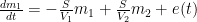
To start off, let’s review the argument I made, which is that the atmospheric-carbon-dioxide turnover time is what determined how long the post-bomb-test excess-carbon-14 level took to decay. That argument was based on the “bathtub” model, which Fig. 1 depicts. The rate at which the quantity <i>m</i> of water the tub contains changes is equal to the difference between the respective rates <i>e</i> (emissions) and <i>u</i> (uptake) at which water enters from a faucet and leaves through a drain:

The same thing can, <i>mutatis mutandis</i>, be said of contaminants (read carbon-14) in the water. But in the case of well-mixed contaminants one of the <i>mutanda</i> is that the rate at which the contaminants leave is dictated by the rate at which water leaves:

where 

Consequently, if the water quantity increases for an interval during which <i>e</i> exceeds <i>u</i>, it will thereafter remain elevated if the emissions rate <i>e</i> then falls no lower than the drain rate <i>u</i>. If a dose of contaminants is added to the water, though, the resultant contaminant amount falls, even when there’s no difference between <i>u</i> and <i>e</i>, in accordance with the <i>turnover</i> rate, i.e., with the ratio of <i>u</i> to <i>m</i>. So, to the extent that this model reflects reality’s relevant aspects, we can conclude that the rate at which the carbon-14 concentration decays tells us nothing about what happens when total-CO2 emissions return to a “normal” level.
But among the foregoing model’s deficiencies is that it says nothing about a possible dependence of overall drain rate <i>u</i> on the water quantity <i>m</i>, whereas we may expect biosphere uptake (and emissions) to respond to the atmosphere’s carbon-dioxide content. Nor does it deal with the possibility that after contamination has flowed out the drain it will be recycled through the faucet. In contrast, the biosphere no doubt returns to the atmosphere at least some of the carbon-14 it has previously taken from it.

A model that takes such factors into account could support a conclusion different from the one to which the bathtub led us. Consistently with my last post’s approach, Fig. 2 uses interconnected pressure vessels to represent one such model. In this case there are only two vessels, the left one representing the atmosphere and the right one representing carbon sinks such as the ocean and the biosphere.
The vessels contain respective quantities 


Those equations tell us that the carbon quantity 
![m_1(t) = \left[ \frac{V_1}{V_1+V_2}+\frac{V_2}{V_1+V_2} \exp\left(-\frac{V_1+V_2}{V_1V_2}St \right)\right] m_0 ,](https://s0.wp.com/latex.php?latex=m_1%28t%29+%3D+%5Cleft%5B+%5Cfrac%7BV_1%7D%7BV_1%2BV_2%7D%2B%5Cfrac%7BV_2%7D%7BV_1%2BV_2%7D+%5Cexp%5Cleft%28-%5Cfrac%7BV_1%2BV_2%7D%7BV_1V_2%7DSt+%5Cright%29%5Cright%5D+m_0+%2C+&bg=ffffff&fg=000&s=0&c=20201002)
which the substitutions 

Note that in the Fig. 2 system any constituent of the gas would be exchanged between vessels in accordance with the partial-pressure difference of that constituent alone, as if it were the only component the vessels contained. By thus constraining the flow from (and to) the first, atmosphere-representing vessel, this model supports the conclusion that the overall-carbon-dioxide quantity would, contrary to my previous argument, decay just as the excess, bomb-caused quantity of atmospheric carbon-14 did.

Could providing more than one sink enable us to escape that conclusion? Not necessarily. Consider the more-complex system that Fig. 3 depicts. Just as the system that my previous post described, this one can embody the TAR Bern-model parameters. As that post indicated, describing such a system requires a fourth-order linear differential equation. So that system does have more degrees of freedom in its initial conditions and can therefore exhibit a wider range of responses.
But it still constrains the flow among its four vessels linearly in accordance with partial pressures, just as the Fig. 2 system does. From complete equilibrium, therefore, its behavior for any constituent is the same as for any other constituent as well as for the contents as a whole. In other words, this model, too, seems to support the notion that the bomb-test results do indeed tell us how long excess carbon dioxide will remain if we stop taking advantage of fossil fuels.
In a sense, though, the models of Figs. 2 and 3 beg the question; they use the same uptake- and emissions-process-representing
So one question is how significant that difference is in the present context. I don’t have the answer, although my guess is, not very. But readers attempting to answer that question could do worse than start by referring to a previous WUWT post by Ferdinand Engelbeen.

Another way in which carbon-14 differs from the other two carbon isotopes is that it’s unstable. So, if the Fig. 3 model is adequate for carbon-12 or -13, a different model, which Fig. 4 depicts, would have to be used for carbon-14 if its radioactive decay is significant. That diagram differs from Fig. 3 in that it includes a flow 
To the extent that those different models produce different responses, using bomb-test data to predict the total carbon content’s behavior is problematic. But the Engelbeen post mentioned above seems to say that even deep-ocean residence times tend to be only a minor fraction of carbon-14’s half-life: this factor’s impact may be small.
A possibly more-significant factor is that the carbon cycle is undoubtedly non-linear, whereas the conclusions we tentatively drew from the models above depend greatly on their linearity. Before I reach that issue, though, I should point out an aspect of the Bern model that was not relevant to my previous post. The Bern equations I set forth in my last post were indeed linear. But that does not mean that their authors meant to say that the carbon cycle itself is. Although for the sake of simplicity I’ve discussed the models’ physical quantities as though they represented, e.g., the entire mass of carbon in a reservoir, their authors no doubt intended their (linear) models’ quantities to represent only the differences from some base, pre-industrial values. Presumably the purpose was to limit their range enough that the corresponding real-world behavior would approximate linearity.
But such linearization compromises the conclusions to which the models of Figs. 2 and 3 led us. A linear system is distinguished by the fact that its response to a composite stimulus always equals the sum of its individual responses to the stimulus’s various constituents; if the stimulus equals the sum of a step and a sine wave, for example, the system’s response to that stimulus will equal the sum of what its respective responses would have been to separate applications of the step and the sine wave. And this “superposition” property was central to drawing the conclusions we did from those models: the response to a large stimulus is proportionately the same as the response to a small one.

To appreciate this, consider Fig. 5, which depicts scaled values of the Fig. 2 model’s left-vessel total-carbon and carbon-14 contents. Initially, the system is at equilibrium, with zero outside emissions 


At time t = 5, a bolus of carbon-14 appears in the (atmosphere-representing) left vessel. Compared with the total carbon content, the added quantity is tiny, but it is large enough to double the small existing carbon-14 content. As the distance between the red dotted vertical lines shows, the resultant increase in carbon-14 content decays toward its new equilibrium value with a time constant of just about seven years. (I’ve assumed that the processes greatly favor the sink-representing right vessel—i.e., that its “volume” is much greater than the left vessel’s—so that the new equilibrium value is not much greater than the original.)
Now consider what happens at t = 45, when the left vessel’s total-carbon quantity suddenly increases. Although the two quantities are scaled to their respective initial values, this total-carbon increase is orders of magnitude greater than the t = 5 carbon-14 increase. Yet, as the black dotted vertical lines show, the decay of the left vessel’s total-carbon content proceeds just as fast proportionately as the much-smaller carbon-14 content did. As was observed above, this could tempt one to conclude that the carbon-14 decay we’ve observed in the real world tells us how fast the atmosphere would respond to our discontinuing fossil-fuel use.
![clip_image009[1]](http://wattsupwiththat.files.wordpress.com/2013/12/clip_image0091.png?quality=75 "clip_image009[1]")
But now consider what can happen if we relax the linearity assumption. Specifically, let’s say that the Fig. 2 model’s proportionality “constant”

In that plot, the red lines show that the carbon-14 decay occurs just as fast as in the previous plot, the carbon-14 content falling to exp(-1) above its new equilibrium value in around seven years. But the much-larger total-carbon increase brings the system into a lower-efficiency range, so that quantity subsides at a more-leisurely pace, taking over forty years. If such results are any indication, bomb-test results are a poor predictor of how long total-carbon content will settle.
Now permit me a digression in which I attempt to forestall pointless discussion of precisely what the quantities are that the graphs show. I believe the exposition is clearest if it is directed, as in Figs. 5 and 6, to ratios that carbon 14 and total carbon bear to their own initial values. But it appears customary to express the carbon-14 content instead in terms of its ratio to total carbon content. This means that, since total carbon has been increasing, the numbers commonly used in carbon-14 discussions could fall below the pre-bomb values, even though total carbon-14 has in fact increased.
For the sake of those to whom that issue looms large, I have attached Fig. 7 to illustrate how the values for carbon-14 itself could differ from those of its ratio to total carbon in a situation in which new (carbon-14-depleted) carbon is continually injected into the atmosphere.

But that’s a detail. More important is the issue that Fig. 6 raises.
Now, I “cooked” Fig. 6’s numbers to emphasize the point that nonlinearity can undermine conclusions based on linear models. Specifically, Fig. 6 depicts the results of making the flows proportional only to the fifth root of the carbon content.
But non-linearity must have some effect. How much? I don’t know. Together with the differences in behavior between carbon-14 and its stable siblings, though, it is among the considerations to take into account in assessing how informative the bomb-test data are.
As I warned at the top of the post, this post draws no conclusions from these considerations. But maybe the foregoing analysis will prompt knowledgeable readers’ comments that help narrow the issues.
Discover more from Watts Up With That?
Subscribe to get the latest posts sent to your email.
Myrrh says:
December 17, 2013 at 6:39 pm
and as volcanic CO2 contributions are effectively indistinguishable from industrial CO2 contributions
Most volcanoes (all subduction volcanoes and many of the deep magma volcanoes) have δ13C levels between -8 and +2 per mil. Any substantial extra release from that source would INcrease the δ13C level of the atmosphere, which is currently at -8.2 per mil and fast decreasing in ratio with human emissions, which are at -24 per mil.
A geologist who doesn’t know that needs to look again at his course books…
The largest eruption in the past decades was the Pinatubo, emitting a factor 100 times the amounts of CO2 etc. of an average volcano. Not even measurable in the atmosphere: even a drop of the CO2 increase rate caused by the drop in temperature.
Thus if you have any indication that a lot of volcanoes are emitting more and more CO2 at the same moment that humans also emitted more and more CO2, then you may have a story. Until then it is just attempts to divert the attention from human emissions, which are the real cause of the increase…
@ferdinand meeus
“What rain is doing is some of the extra CO2 releases bringing back to the surface.”
To me that does not add up, though you have stated the idea clearly. The idea falters on the concept that the warm oceans are a net source, not a net sink of CO2. There are so many buffering options awaiting the arrival of enough CO2 that I will remain skeptical that rain, with a high CO2 content, falling from all sorts of heights, is merely cycling back to the ocean what just emerged from it. For a start this cycle should be represented in common pictograms of the carbon cycle. It is a significant path and it is in addition to air-water exchanges. That is not a whinge at you, it is a whinge at the oversimplification of the processes at work.
When cold rain falls on cold seas, there is a net uptake, agreed? The North Atlantic comes to mind. All that rain is carrying CO2 into the oceans at a rate well above the supposed air-water exchange. I have seen in articles the claim that the surface area Is a limiting factor, but the rain path is never considered even though it exceeds it.
“Most of it is simply recycling and one the main CO2 flows still is from the equator to the poles via the atmosphere and back via the deep oceans: ~40 GtC/yr.”
I am pretty sure this contradicts the claims made about where the CO2 comes from north of 60. I don’t have an opinion on that. I didn’t calculate it yet. Just observing.
“Other fluxes are mainly seasonal between ocean surface and atmosphere (~50 GtC back and forth) and between vegetation and atmosphere (~60 GtC back and forth) . Human emissions are ~10 GtC/yr and the carbon circulating through the water vapour cycle is ~0.5 GtC/yr.”
You have omitted the cycling of CO2 into and out of atmospheric water droplets, and in fact the whole cryosphere. Ice and snow contain virtually no CO2 at all – that I checked ad nauseum. There is nothing left to find. Ice expels CO2 and in NH winter, the cryosphere kicks out a great deal – enough to move the pointer up 5 ppm. I remember many years ago a warmista blaming the winter rise on fossil fuel burning in cold countries!!
The CO2 released from ice and snow is circulated SOUTH in NH winter and is detectable in Hawaii. Right now the mass of ice and snow is building rapidly, and the CO2 thus liberated is diffusing southward on ‘polar winds’. This is part of the water vapour cycle so I sincerely doubt the figure of ‘~0.5 GtC/yr’. If you want to express it in terms of C and not CO2, it is closer to ~10 GtC/yr or 20 times as much as is commonly assumed. In my view the hydrosphere and cryosphere are very poorly considered in models of the carbon cycle, which is odd given the propensity for water to absorb, and ice to release, CO2.
One of the easiest ways to consider the amount of CO2 passing through the systems is that the pH of rain is about ~5.6 (as a poster noted above) and the pH of the ocean is ~8.1. The ocean processes (life) gobbles it up and gives back what else it can’t hold, if it didn’t sink out of sight. That is not cycling the same CO2 round and round using rain. Rain pumps CO2 down.
Crispin in Waterloo says:
December 18, 2013 at 7:18 am
One of the easiest ways to consider the amount of CO2 passing through the systems is that the pH of rain is about ~5.6 (as a poster noted above) and the pH of the ocean is ~8.1. The ocean processes (life) gobbles it up and gives back what else it can’t hold, if it didn’t sink out of sight. That is not cycling the same CO2 round and round using rain. Rain pumps CO2 down.
The pH is related to the presence of buffers not the concentration of CO2, seawater absorbs more CO2 than freshwater.
Crispin
The idea falters on the concept that the warm oceans are a net source, not a net sink of CO2.
The upwelling zones in the equator bring oversaturated seawater from the cold deep up to the surface, where it warms and releases a lot of CO2, quantified some 40 GtC that is circulating through the atmosphere and the deep oceans.
The pCO2 of the warm oceans is measured and shows high levels, a lot higher than in the atmosphere:
http://www.pmel.noaa.gov/pubs/outstand/feel2331/mean.shtml
(BTW, the 2.2 GtC/yr absorbed by the oceans they mention is the net uptake, not how much circulates.)
pH is certainly an important factor in the amounts of CO2 that can be absorbed by the ocean waters vs. fresh water. But it is exactly the low pH which is the result of the dissolution of CO2 into bicarbonate/carbonate and hydrogen ions that makes that the solubility of CO2 in fresh water is quite low.
All what the large surface of raindrops do is increasing the speed with which the equilibrium between CO2 in air and water is reached, but it doesn’t change the total amount absorbed: that depends of the total amount of water, its temperature and the partial pressure of CO2 in the atmosphere.
The maximum is 1.32 mg/liter at near freezing and 0.0004 bar CO2 in the atmosphere, that really is all and much lower than you expect…
I don’t think that the cryosphere is the main source of the increase in the atmosphere: the 13C/12C ratio changes too, which points to more release from decaying vegetation than from the oceans or the cryosphere. The decay of organic debris goes on even in mid-winter from under the snowdeck…
@Phil. says:
>The pH is related to the presence of buffers not the concentration of CO2, seawater absorbs more CO2 than freshwater.
Yes I am aware of that and didn’t feel a need to repeat it or get into the total CO2 v.s. the total free CO2. I am of course referring to the CO2 solvated in the water/sea water.
@ferdinand meeus: I am aware that you and many other do not consider the cryosphere is a major or the main source of CO2. The 13C/12C argument is not convincing, however. The decaying of organic vegetation carries on in water as well but is stunted greatly by freezing. (There are a few papers available on Alaskan CO2 and CH4 emissions from decaying tundra.) I would be most interested in seeing some proof of a detectable seasonal change in the ratio and the cause of that change. My numbers show that the cessation of vegetative growth in winter is not sufficient to explain the large rise in CO2. Certainly half of it, at least, seems to come from freezing water. When the ice melts the water reabsorbs CO2. The CO2 concentration line follows the ice timeline better than the area of vegetative growth. Check it out.
The implication is significant: if large ice masses are melted, the resulting water, either fresh of salt, will absorb a large amount of CO2. I believe models do not include this basic fact. ‘Melt’ 1/4 of the ice on Antarctica and see what you calculate. Add Greenland’s ice sheet. It’s a lot.
Crispin in Waterloo says:
December 18, 2013 at 8:17 pm
Here the seasonal CO2 and δ13C changes from Barrow and Mauna Loa:
http://www.ferdinand-engelbeen.be/klimaat/klim_img/seasonal_CO2_d13C_MLO_BRW.jpg
averages are from 1990-2012, each year is zeroed for the January values.
Barrow is most of the year a frozen area, except during the short summer. Despite the huge melt/refreeze of ice in its neighbourhood, the main change in CO2 is accompanied by a main change in δ13C which points to vegetation as main cause of the variation.
There is hardly any seasonal change in the SH, neither much δ13C change. That means that sea ice freezing and thawing doesn’t play much role in the CO2 burget.
While I am familiar with that data, I need some time to read through that and consider the implications of the δ13C change. There are two profs I want to consult with before responding. The CO2 level at Point Barrow (there is a WUWT correspondent there) is strongly correlated with freezing/melting ice which your chart shows so I want to consider how that influences that you conclude. The Barrow local concentration is an exaggerated version of the Mauna Loa change which I consider an important indicator. Someone on another thread suggested that the freezing of the ice caps the oceans and the CO2 piles up waiting for spring. On a mass basis sea water contains roughly 0.6 kg per cubic metre (solvated) or about 400 ppm(v). Agreed or not? Adjust as necessary.
The Arctic sea ice alone requires freezing enough water to expel about 20 gigatons of CO2. There is a heck of a lot more frozen water that just the sea ice in an NH winter. A while ago a correspondent suggested the CO2 goes into the sea water ‘as it cools’ but the Arctic sea water doesn’t cool meaningfully. The ice is heated from below, not above.
My motto is ‘never assume anything’. I will return to this topic one another thread. I have nothing substantial to add at this time. I want to read a bit on δ13C which is absorbed preferentially by some sea and land plants. You say the main variation is caused by vegetation, but we were also assured not that long ago the CO2 rise in winter was caused by human emissions from fossil fuels. It is contributory but minimal. I would like to know if fresh water or things in it preferentially take up δ12C. Many things are possible, which is why bananas are ‘radioactive’.
Thanks
C
Crispin in Waterloo says:
December 19, 2013 at 10:14 am
The Arctic sea ice alone requires freezing enough water to expel about 20 gigatons of CO2. There is a heck of a lot more frozen water that just the sea ice in an NH winter. A while ago a correspondent suggested the CO2 goes into the sea water ‘as it cools’ but the Arctic sea water doesn’t cool meaningfully. The ice is heated from below, not above.
One point, once the surface ice forms, any ice which forms underneath has no route to expel the CO2 to the atmosphere, so it must either remain in the form of bubbles in the ice or dissolve in the seawater below the ice
I had thought something similar, Phil. Presumably an extra amount of CO2/bicarbonate-rich brine flows downwards? And would this also increase as the annual FLUX of sea ice increases (i.e. as more sea-ice melts in summer, a larger amount of fresh sea-ice forms in winter)?