Models Fail: Greenland and Iceland Land Surface Air Temperature Anomalies

I’m always amazed when global warming enthusiasts announce that surface temperatures in some part of the globe are warming faster than simulated by climate models. Do they realize they’re advertising that the models don’t work well for the area in question? And that their shouting it from the hilltops only helps to highlight the limited value of the models?

Greenland is a hotspot for climate change alarmism in more ways than one. A chunk of glacial ice sits atop Greenland, and as it melts, it contributes to the rise in sea levels. If surface temperatures in Greenland warm in the future, the warming rate will impact how quickly Greenland ice melts and its contribution to future sea levels. Greenland is also one of the locations around globe where land surface air temperatures in recent decades have been warming faster than simulated by models. See Figure 1, which is a model-data comparison of the surface air temperature anomalies of Greenland and its close neighbor Iceland. Somehow, that modeling failure turns into proclamations of doom, with the Chicken Littles of the anthropogenic global warming movement proclaiming we’re going to drown because rising sea levels.

Figure 1

Figure 1

A more detailed discussion of Figure 1: It compares the new and improved UK Met Office CRUTEM4 land surface air temperature anomalies for Greenland and Iceland (60N-85N, 75W-10W), for the period of January 1970 to February 2013, and the multi-model ensemble-member mean of the models stored in the CMIP5 archives, based on the scenario RCP6.0. As you’ll recall, the models in the CMIP5 archive are being used by the IPCC for its upcoming 5th Assessment Report. Based on the linear trends, since 1970, Greenland and Iceland surface air temperatures are warming at a rate that’s about 65% faster than predicted by the models. That’s not a very good showing for the models. And, for example, the disparity between the models and observations is even greater if we start the comparison in 1995, Figure 2. During the last 18 years, Greenland and Iceland land surface temperatures have been warming at a rate that’s more than 2.5 times faster than simulated by models. Obviously the modelers haven’t a clue about what causes land surface temperatures to warm there.

Figure 2

Figure 2

LOOKING AT THE RECENT WARMING PERIOD DOESN’T TELL THE WHOLE STORY

The data in Figure 1 covers a period of a little more than 40 years. Let’s look at a model-data comparison for the 40-year period before that, January 1930 to December 1969. Refer to Figure 3. During that multidecadal period, land surface air temperature anomalies in Greenland and Iceland actually cooled, and they cooled at a significant rate. On the other hand, the models show a miniscule long-term cooling from 1930 to 1969, but the trend is basically flat. The models fail again.

Figure 3

Figure 3

In our example in Figure 2, we looked at the trends from 1995 to present, so Figure 4 compares the models and data from January 1930 to December 1994. The data show cooling at a significant rate, about 0.25 deg C per decade, but now the models show warming.
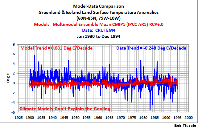
Figure 4

Figure 4

TWO MORE REASONS FOR THIS EXERCISE

In addition to showing you how poorly the models simulate the land surface temperatures of Greenland and Iceland, another point I wanted to make was that you have to be wary of the start year of any study of Greenland surface temperatures. Figure 5 compares the models and data for Greenland and Iceland from 1930 to present. In it, the data and model output have been smoothed with 13-month running-average filters to minimize the monthly variations. Greenland and Iceland obviously cooled for much of the period since 1930. The break point between cooling and warming is probably debatable. But the most outstanding feature in the data is the extreme dip and rebound in the early 1980s. That dip appears about the time of the eruption of El Chichon in Mexico, and there’s another dip in 1991, which is when Mount Pinatubo erupted. Mount Pinatubo was a stronger eruption, so the 1982 dip appears unusual. Bottom line: keep in mind that any study of the recent warming of Greenland and Iceland surface temperatures will be greatly impacted by the start year.
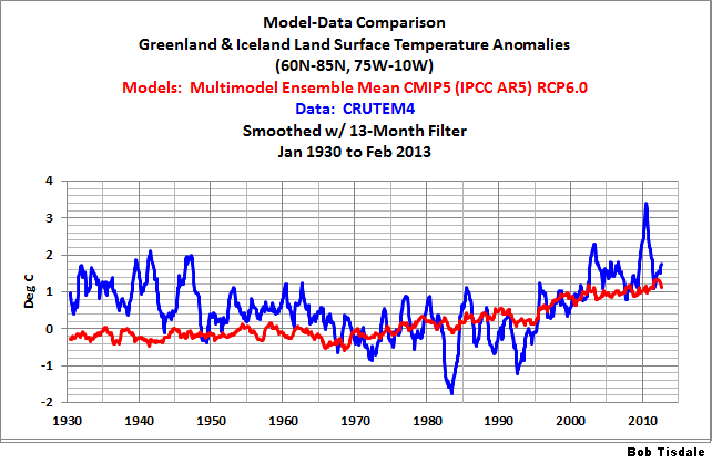
Figure 5

Figure 5

The other point: Based on the linear trends (of the monthly data not the illustrated smoothed versions), land surface air temperature anomalies for Greenland and Iceland have not warmed since 1930. See Figure 6. Phrased another way, Greenland and Iceland surface temperatures have not warmed in 80+ years. But the models show they should have warmed about 1.3 deg C during that time. Granted, land surface temperatures now are warmer than then were in the 1930s and ’40s, but the models can’t simulate the cooling that took place from the 1930s to the latter part of the 20th Century, and they can’t be used to explain the recent warming.

Figure 6

Figure 6

Again, the models show no skill at being able to simulate surface temperatures. No skill at all. Even for critical locations like Greenland.

STANDARD BLURB ABOUT THE USE OF THE MODEL MEAN

We’ve published numerous posts that include model-data comparisons. If history repeats itself, proponents of manmade global warming will complain in comments that I’ve only presented the model mean in the above graphs and not the full ensemble. In an effort to suppress their need to complain once again, I’ve borrowed parts of the discussion from the post Blog Memo to John Hockenberry Regarding PBS Report “Climate of Doubt”.

The model mean provides the best representation of the manmade greenhouse gas-driven scenario—not the individual model runs, which contain noise created by the models. For this, I’ll provide two references:

The first is a comment made by Gavin Schmidt (climatologist and climate modeler at the NASA Goddard Institute for Space Studies—GISS). He is one of the contributors to the website RealClimate. The following quotes are from the thread of the RealClimate post Decadal predictions. At comment 49, dated 30 Sep 2009 at 6:18 AM, a blogger posed this question:

If a single simulation is not a good predictor of reality how can the average of many simulations, each of which is a poor predictor of reality, be a better predictor, or indeed claim to have any residual of reality?

Gavin Schmidt replied with a general discussion of models:

Any single realisation can be thought of as being made up of two components – a forced signal and a random realisation of the internal variability (‘noise’). By definition the random component will uncorrelated across different realisations and when you average together many examples you get the forced component (i.e. the ensemble mean).

To paraphrase Gavin Schmidt, we’re not interested in the random component (noise) inherent in the individual simulations; we’re interested in the forced component, which represents the modeler’s best guess of the effects of manmade greenhouse gases on the variable being simulated.

The quote by Gavin Schmidt is supported by a similar statement from the National Center for Atmospheric Research (NCAR). I’ve quoted the following in numerous blog posts and in my recently published ebook. Sometime over the past few months, NCAR elected to remove that educational webpage from its website. Luckily the Wayback Machine has a copy. NCAR wrote on that FAQ webpage that had been part of an introductory discussion about climate models (my boldface):

Averaging over a multi-member ensemble of model climate runs gives a measure of the average model response to the forcings imposed on the model. Unless you are interested in a particular ensemble member where the initial conditions make a difference in your work, averaging of several ensemble members will give you best representation of a scenario.

In summary, we are definitely not interested in the models’ internally created noise, and we are not interested in the results of individual responses of ensemble members to initial conditions. So, in the graphs, we exclude the visual noise of the individual ensemble members and present only the model mean, because the model mean is the best representation of how the models are programmed and tuned to respond to manmade greenhouse gases.

CLOSING

Will the warming continue in Greenland and Iceland? If so, for how long? Or will the surface temperatures in Greenland and Iceland undergo another multidecadal period of cooling in the near future? The models show no skill at being able to simulate land surface air temperatures in Greenland and Iceland, so we can’t rely on them for predictions of the future.

We can add the surface temperatures of Greenland and Iceland to the growing list of climate model failures. The others included:

Scandinavian Land Surface Air Temperature Anomalies

Alaska Land Surface Air Temperatures

Daily Maximum and Minimum Temperatures and the Diurnal Temperature Range

Hemispheric Sea Ice Area

Global Precipitation

Satellite-Era Sea Surface Temperatures

Global Surface Temperatures (Land+Ocean) Since 1880

And we recently illustrated and discussed in the post Meehl et al (2013) Are Also Looking for Trenberth’s Missing Heat that the climate models used in that study show no evidence that they are capable of simulating how warm water is transported from the tropics to the mid-latitudes at the surface of the Pacific Ocean, so why should we believe they can simulate warm water being transported to depths below 700 meters without warming the waters above 700 meters?

I’ve got at least one more model-data post, and it’s about the land surface temperatures of another continent. The models almost double the rate of warming there.

Looks like I’ve got a lot of ammunition for my upcoming show and tell book. It presently has the working title Climate Models are Crap with the subtitle An Illustrated Overview of IPCC Climate Model Incompetence.

It’s unfortunate that the IPCC and the government funding agencies were only interested in studies about human-induced global warming. They created their consensus the old fashioned way: they paid for it. Now, the climate science community is still not able to differentiate between manmade warming and natural variability. They’re no closer to that goal than they were when they formed the IPCC. Decades of research efforts and their costs have been wasted by the single-sightedness of the IPCC and those doling out research funds.

They got what they paid for.

0 0 votes
Article Rating
78 Comments
Oldest
Newest Most Voted
Inline Feedbacks
View all comments
July 6, 2013 7:20 am

Gavin Schmidt replied with a general discussion of models:
Any single realisation can be thought of as being made up of two components – a forced signal and a random realisation of the internal variability (‘noise’). By definition the random component will uncorrelated across different realisations and when you average together many examples you get the forced component (i.e. the ensemble mean).
===============
Climate models represent weather over time. The variability in weather is not noise, it is chaos. While chaos appears random, it is not. You cannot average chaos to get the forced component.
This is why the ensemble mean is worthless as a prediction of future climate. As time increases the chaotic component of the signal does not average to zero as does random noise. Rather, it causes the temperature to vary unpredictably, making is impossible to separate the forced components from the chaotic components.

Roberto
July 6, 2013 7:26 am

In most statistics, one of the most important things you have to publish is the significance of the measurements. Nobody says “this is significant” without saying HOW significant. How was that statement validated?
The same with normal computer models. You validate them again and again. You don’t go around saying they passed or they failed without having the data to show HOW they passed or failed. The test cases. Precisely what did the model say, and how well was that supposed to match reality? What were the criteria?
I can’t imagine a computer professional who doesn’t know that and live it.
But the alarmist fans have a clearly non-normal approach. “These models are marvelous”, with little clue how they know that or how marvelous they are supposed to be before we trust them.

July 6, 2013 7:32 am

The climate model do however have value when interpreted correctly. What the spaghetti graph of climate models does demonstrate is the natural variability of the system. The models are telling us that due to natural variability alone, any one of the many, many different results are possible, and there is no way to know which one will actually occur.
What the spaghetti graph of climate models shows is that due to natural variability alone, we may get wide increases or decreases in temperature, with the identical forcings. This variability however is not “noise”, it is chaos. Thus, the reliability of the mean does not improve over time.

July 6, 2013 7:45 am

Roberto says:
July 6, 2013 at 7:26 am
I can’t imagine a computer professional who doesn’t know that and live it.
============
Commercial software lives and dies depending on whether its results match the NEEDS of its customers. Academic software however lives and dies depending on how well its results match the BELIEFS of those controlling the grant monies.
Thus, commercial software requires validation to ensure that it is working correctly. However, in academic software such validation will work against you if the beliefs of those controlling the grant monies do not match reality. Thus, there is no value in validating academic software and good reasons not to.

Editor
July 6, 2013 7:52 am

ferd berple says:
July 6, 2013 at 7:32 am

The climate model do however have value when interpreted correctly. What the spaghetti graph of climate models does demonstrate is the natural variability of the system. The models are telling us that due to natural variability alone, any one of the many, many different results are possible, and there is no way to know which one will actually occur.

Unless there’s code in the models that tries to model that natural variablility, I’d argue that the models are merely showing the chaotic behavior of what they do model.
Once they are better at modeling things like the PDO, the NAO, and water vapor to cloud transitions, and everything else that makes up “natural variability” then I might agree they’re modeling that. Until then, I see that phrase more as a screen for things the modelers don’t understand than something visible in model output.

Jim G
July 6, 2013 7:52 am

“And that their shouting it from the hilltops only helps to highlight the limited value of the models?”
Mr. Berple has put his finger upon the real issue. Climate is a multivariate chaotic system and “limited value” is a vast overstatement with regards to value of existing models of same. Their abuse of statistics is monumental.

July 6, 2013 8:02 am

Eyeballing figure 6 tells me that the model results are completely different to the data.
The models and data are just two wiggly lines laid one on top of the other – they don’t match at all.
Bob’s right: the models are cr*p

Alaska Mike
July 6, 2013 8:26 am

Bob Tisdale:
Figure one and two show data through 2013. Why was figure four cutoff at 1995? If you have the data why not show it through the present date?

noaaprogrammer
July 6, 2013 9:01 am

The core algorithm for simulating future climate should be the random walk of a drunk.

William Astley
July 6, 2013 9:02 am

I fully support the scientific logic of this thread. Increases in atmospheric CO2 are evenly distributed in the atmosphere. The potential for CO2 forcing due to the increase in atmospheric CO2 should therefore be more or less equal by latitude. As the actual amount of warming due to the CO2 increase should be proportional to the amount of emitted radiation at the latitude in question, the greatest amount of warming due to the CO2 mechanism should be in the tropics. That is not observed. The latitude pattern of warming does not match the signature of the CO2 forcing mechanism.
To explain the observed latitudinal pattern of warming – ignoring the second anomaly that there has been no warming for 16 years which requires a smart mechanism to turn off the CO2 forcing mechanism or suddenly to hid the CO2 forcing energy imbalance – using the CO2 forcing mechanism there would need to be a smart natural forcing mechanism that would inhibit warming in the tropics and amplify warming in other latitudes.
The observed warming in the last 70 years is not global, evenly distributed. What is observed is the most amount of warming is in the Northern hemisphere at high latitudes (The Northern hemisphere has warmed twice as much warming as the global as whole and four times as much warming as the tropics). The idiotic warmists ignore the fact that the latitudinal pattern of warming disproves their hypothesis and the no warming for 16 also invalidates the modeling of the CO2 mechanism and their assertion that the majority of the 20th century warming was caused by CO2. The warmists are not interested in solving a scientific problem, therefore any warming is good enough to support CO2 warming. AGW is being used to push the green parties’ and green NGO’s political agenda which is a set of very expensive scams.
Fortunately or unfortunately CO2 is not the primary driver of climate. Clouds in the tropics increase or decrease to resist forcing change by reflecting more or less sunlight off into space. Super cycle changes to the solar magnetic cycle are the driver of both the 1500 year warming/cooling cycle and the Heinrich abrupt climate events that initiate and terminate interglacials.
The warmists also ignore the fact that the same warming pattern that we are now observing has occurred cyclically in the past and the past cycles correlate with solar magnetic cycle changes. Ironically, if significant global cooling and crop failures’ ending the climate wars is considered to be ironic rather than tragic, the sun is rapidly heading to a deep Maunder like minimum. The planet is going to cool. The physics of past and future climate change is independent of the climate wars and incorrect theories. Greenland ice temperature, last 11,000 years determined from ice core analysis, Richard Alley’s paper.
http://www.climate4you.com/images/GISP2%20TemperatureSince10700%20BP%20with%20CO2%20from%20EPICA%20DomeC.gif
http://www.solen.info/solar/images/comparison_recent_cycles.png
Gavin Schmidt also stated that if the planet did not amplify forcing changes and CO2 has not the primary driver of climate that climatologists could not explain the glacial/interglacial cycle.
Gavin Schmidt needs to read through the following books. (Unstoppable warming every 1500 years or so is of coursed followed by unstoppable cooling when the sun enters a deep Maunder like minimum.)
http://www.amazon.com/Unstoppable-Global-Warming-Updated-Expanded/dp/0742551245
http://www.amazon.com/dp/1840468661
Limits on CO2 Climate Forcing from Recent Temperature Data of Earth
The global atmospheric temperature anomalies of Earth reached a maximum in 1998 which has not been exceeded during the subsequent 10 years (William: 16 years and counting).
…1) The atmospheric CO2 is slowly increasing with time [Keeling et al. (2004)]. The climate forcing according to the IPCC varies as ln (CO2) [IPCC (2001)] (The mathematical expression is given in section 4 below). The ΔT response would be expected to follow this function. A plot of ln (CO2) is found to be nearly linear in time over the interval 1979-2004. Thus ΔT from CO2 forcing should be nearly linear in time also. … ….2) The atmospheric CO2 is well mixed and shows a variation with latitude which is less than 4% from pole to pole [Earth System Research Laboratory. 2008]. Thus one would expect that the latitude variation of ΔT from CO2 forcing to be also small. It is noted that low variability of trends with latitude is a result in some coupled atmosphere-ocean models. For example, the zonal-mean profiles of atmospheric temperature changes in models subject to “20CEN” forcing ( includes CO2 forcing) over 1979-1999 are discussed in Chap 5 of the U.S. Climate Change Science Program [Karl et al.2006]. The PCM model in Fig 5.7 shows little pole to pole variation in trends below altitudes corresponding to atmospheric pressures of 500hPa.
If the climate forcing were only from CO2 one would expect from property #2 a small variation with latitude. However, it is noted that NoExtropics is 2 times that of the global and 4 times that of the Tropics. Thus one concludes that the climate forcing in the NoExtropics includes more than CO2 forcing… ….Models giving values of greater than 1 would need a negative climate forcing to partially cancel that from CO2. This negative forcing cannot be from aerosols. …
These conclusions are contrary to the IPCC [2007] statement: “[M]ost of the observed increase in global average temperatures since the mid-20th century is very likely due to the observed increase in anthropogenic greenhouse gas concentrations.”
http://www-eaps.mit.edu/faculty/lindzen/236-Lindzen-Choi-2011.pdf
On the Observational Determination of Climate Sensitivity and Its Implications Richard S. Lindzen1 and Yong-Sang Choi2
http://icecap.us/images/uploads/DOUGLASPAPER.pdf
A comparison of tropical temperature trends with model predictions
We examine tropospheric temperature trends of 67 runs from 22 ‘Climate of the 20th Century’ model simulations and try to reconcile them with the best available updated observations (in the tropics during the satellite era). Model results and observed temperature trends are in disagreement in most of the tropical troposphere, being separated by more than twice the uncertainty of the model mean. In layers near 5 km, the modelled trend is 100 to 300% higher than observed, and, above 8 km, modelled and observed trends have opposite signs. These conclusions contrast strongly with those of recent publications based on essentially the same data.

LT
July 6, 2013 9:08 am

Without removing El-Chichon and Pinatubo effects you cannot say for sure what the real trend is

D. J. Hawkins
July 6, 2013 9:15 am

Bob Tisdale;
avast! is flagging your e-mail as carrying some malware. Don’t know if it’s something hinky with avast!, but you might want to double check.

D. J. Hawkins
July 6, 2013 9:17 am

Bob Tisdale;
More specifically:
Infection Details
URL: http://bobtisdale.files.wordpress.com/20
Process: C:\PROGRA~1\Google\GOOGLE~1\GOEC62~1.DLL
Infection: URL:Mal

Alan S. Blue
July 6, 2013 9:22 am

Stop comparing ‘trendline to trendline’ smoothed or unsmooothed. The model (or ensembles of models) is a prediction. Compare the least-squared error month-by-month to the actual observations.

July 6, 2013 9:30 am

Iceland’s (Reykjavik) temperatures closely follow ocean currents response to the geo-tectonics; in the winter along Reykjanes Ridge (to the south) and in the summers Kolbeinsey Ridge (to the north), giving decadal predictive or forecasting opportunity. Annual temperatures forecast is obtained by averaging of the above two:
http://www.vukcevic.talktalk.net/RF.htm

Robert Austin
July 6, 2013 10:55 am

ferd berple says:
July 6, 2013 at 7:32 am

The climate model do however have value when interpreted correctly. What the spaghetti graph of climate models does demonstrate is the natural variability of the system.

I can’t say that I agree that climate models have value as predictors of future climate. Perhaps they have some kind of academic value as a kind of “Sim City” exercise in producing the climate of an artificial and fictitious world. The spaghetti graph of multiple climate models does not demonstrate natural variability, it simply shows that the output of different models produces notably differing results. It is the variation in the runs of an individual model that is alleged to show natural variability. So the mean of a number of runs of an individual model perhaps has some meaning as filtering out what the designer thinks as climate noise or natural climate variability. This is totally different from the practice of the ensemble averaging multiple models. Since there is no way of knowing which if any of the climate models is closest in projecting the actual trajectory of empirical data, averaging the results of different models has no actual validity. I guess at best the average of the model ensemble might be construed as the “concensus” of the modelers!

Leo Morgan
July 6, 2013 10:57 am

Could somebody ask a professional on my behalf, what is the expected effect on temperature of Earth’s declining magnetic field?
Just how much energy did the strong field deflect? Is it nothing or is it a significant amount? Did the effect warm the earth’s interior? Are all those charged particles now going into the atmosphere to warm it?
Could the decline in the Earth’s magnetic field be a factor in the underestimate of the warmth of the atmosphere above Greenland and iceland?
P.S. can anyone refer me to a site that analyses the amount we’ve spent on not changing the world’s temperature?

Stephen Rasey
July 6, 2013 11:15 am

Yes, the models don’t match the data in Iceland.
But what is the DATA? How has it been adjusted?
GHCN’s Dodgy Adjustments In Iceland, or what I call The Smoking Shotgun in Iceland. Iceland is the test case that exposes the shenanigans going on is adjustment of temperatures records.
So the real question in Iceland and Greenland is, “Are the ‘Data’ from CRUTEM4 worth anything?” Are they any better than GHCN/GISS? With the initials “CRU…”, I’m skeptical.

Jimbo
July 6, 2013 11:15 am

Here are some paper abstracts showing more rapid or similar rates of warming in Greenland covering the period between 1920 to 1940 as well as one paper which says:

…we conclude that the current decadal mean temperature in Greenland has not exceeded the envelope of natural variability over the past 4000 years,….

All occurred under the ‘safe’ level of co2 at 350ppm.

Jimbo
July 6, 2013 11:18 am

How will Greenland ice sheet respond to the speculated global mean temperature at the end of the century? I don’t have a clue but we can look at the Eemian very warm inter-glacial (warmer than the hottest decade evaaaaah).

(Nature – 2013) “…a modest ice-sheet response to the strong warming in the early Eemian…”
http://www.nature.com/nature/journal/v493/n7433/full/nature11789.html

Paul Penrose
July 6, 2013 11:28 am

I have to agree with Fred here; the ensemble means are meaningless. It is obvious that the individual runs of DIFFERENT models are not single realizations of the same thing, so it is meaningless to average them together. Even averaging individual runs of the same model is questionable. Has anyone even tried to characterize the “noise”? I’ll bet it’s far from a normal distribution. So the whole thing is just an exercise in statistical shenanigans.

Stephen Rasey
July 6, 2013 11:28 am

ferd berple: What the spaghetti graph of climate models does demonstrate is the natural variability of the system.
Robert Austin: The spaghetti graph of multiple climate models does not demonstrate natural variability, it simply shows that the output of different models produces notably differing results.
I side with Robert. The Spaghetti graph at best shows the uncertainty in the mean signal from uncertainty in global alleged physical parameters with attempts to calibrate to the historical data. Show me where the calibration to natural variability exists in the process? We only have one run of the real data, if you discount the various revisions of the historical record.

rogerknights
July 6, 2013 12:47 pm

Looks like I’ve got a lot of ammunition for my upcoming show and tell book. It presently has the working title Climate Models are Crap with the subtitle An Illustrated Overview of IPCC Climate Model Incompetence.

How about “Climola”? (Followed by one or more explanatory subtitles.) This lets you avoid using the word “crap” explicitly, but suggesting it by way of “climola’s” chiming subconsciously with “shinola” and “shinola’s” association with “sh*t”.

rogerknights
July 6, 2013 1:16 pm

Or how about “Garbage Out: The Fruit of the IPCC’s Climate Models”?
Whatever the subtitle, I think that “Garbage Out” is a really “strong” title–it’s a “grabber”–and a winner.
“Fruit” brings to mind the advice to judge the models by their fruits–i.e., the outcome of their predictions (which are garbage).
By further subconscious association, “Garbage Out” suggests “take out the garbage”–i.e., get rid of the models.

July 6, 2013 1:30 pm

More proof that models are worse than useless – they are nothing but a priori constructs fully intended to deceive rather than enlighten, a positive evil.

rogerknights
July 6, 2013 1:34 pm

PS: One last (hah!) tweak:
Garbage Out: The Wormy “Fruit” of the IPCC’s Climate Models
The sneer quotes around Fruit more strongly link it to Garbage and also imply that the word is being used figuratively, as in the Gospels and bringing to mind their advice.
Or maybe here’s another tweak, one that brings to mind the phrase, “Gospel in, Garbage out.”
Garbage Out: The Wormy “Fruit” of the IPCC’s Climate Gospel
The downside of that one is that the word “model” is omitted explicitly. But it may not be necessary to include it, since the whole title suggests it. (But probably this is one tweak too far.)

rogerknights
July 6, 2013 2:15 pm

PPS: Someone has probably used “Garbage Out” as a title already. But book titles aren’t copyrighted. Some titles have been used on as many as eight different books.

Alaska Mike
July 6, 2013 2:22 pm

Bob Tisdale:
Thank you for answering my curiosity of “Why was figure four cutoff at 1995? If you have the data why not show it through the present date?” and steering my attention to your point. I had to re-read your article a second time. I freely admit I’m not the “Sharpest Statistical Tool in the shed,” but I do try. Again, I appreciate your personal note, and everything all contributors do for Anthony and WUWT.
Alaska Mike

Stephen Rasey
July 6, 2013 3:11 pm

I like “Gospel In, Garbage Out” “Gospel” may or may not be the Truth, depending upon your point of view and upbrining, but it is definately the foundation consensus of the sect. It also brings in the religious furvor of CAGW believers. Now, if there was only a way to work in: “Drinking the Climate Change Cool-aid.”

July 6, 2013 3:17 pm

BT: with the Chicken Littles of the anthropogenic global warming movement proclaiming we’re going to drown because rising sea levels.
BPL: I think you underestimate the danger. A city doesn’t have to be underwater to be threatened by rising sea levels. The water only has to get high enough to back up sewers and seep into aquifers. Without sewage disposal, and without fresh water, a city becomes a death trap.
And the rise won’t be perfectly even. It will come in a series of stochastic events–storm surges. Some will flood cities and some won’t.
But you’re right that rising sea level is not the most immediate danger from global warming. That would be agricultural failure due to rising drought in continental interiors.

Scott
July 6, 2013 4:06 pm

If there is localised heating above the Model projection then for the models to be valid given the models main driver, there must be higher CO2 levels in Greenland.
Are there any CO2 measurements in Greenland? because without it they just have an epic fail regardless of what else is happening.

July 6, 2013 6:02 pm

A usually overlooked feature of these IPCC climate models is that they provide no information to a policy maker about the outcomes from his or her policy decisions thus being useless for the purpose of making policy. That they seem to policy makers to be useful for this purpose suggests these policy makers have been deceived through applications of the equivocation fallacy on the part of IPCC climatologists ( see http://wmbriggs.com/blog/?p=7923 for proof ).

Stephen Rasey
July 6, 2013 7:49 pm

That they seem to policy makers to be useful for this purpose suggests these policy makers have been deceived
Who has been deceived?
Policy makers aren’t deceived, but will embrace a model that supports the decision they want.
CBO: Obamacare Will Spend More, Tax More, and Reduce the Deficit Less Than We Previously Thought Forbes: 7/27/’12
No One believed the CBO estimates. But Democrats used it as cover and to shift responsibility for busting the budget.
The same thing is happening with the use of climate models. Policy makers don’t believe the models, but they use the models as a “Get out of Jail” card.

Terry Oldberg
Reply to  Stephen Rasey
July 6, 2013 8:55 pm

Stephen Rasey:
As you suggest, policy makers may not have been deceived by IPCC climatologists. Instead, they may have been a party to this deception. If they did it for money, they were guilty of civil and criminal fraud under the laws of the U.S.

July 6, 2013 7:53 pm

Some of the mistakes made by the IPCC and the Consensus are revealed at http://consensusmistakes.blogspot.com/

Theo Goodwin
July 6, 2013 8:43 pm

Ric Werme says:
July 6, 2013 at 7:52 am
Ric Werme has this right. Let us constrast actual reasoning and Schmidt’s reasoning. In actual reasoning, one might create several models of the flight pattern of migrating geese, average the models, and come up with a “Vee” shape. By contrast, consider Schmidt’s reasoning:
“Any single realisation can be thought of as being made up of two components – a forced signal and a random realisation of the internal variability (‘noise’). By definition the random component will uncorrelated across different realisations and when you average together many examples you get the forced component (i.e. the ensemble mean).”
All this says is that the several scatter diagrams will reveal the “correct shape” after they are averaged. The models have to be about something. And the average of the scatter diagrams have to reveal some thing that was hypothesized in all the models. In other words, we need some geese, some pictures of them migrating, and so on. As Ric says:
“Once they are better at modeling things like the PDO, the NAO, and water vapor to cloud transitions, and everything else that makes up “natural variability” then I might agree they’re modeling that. Until then, I see that phrase more as a screen for things the modelers don’t understand than something visible in model output.”
Finally, as ferd berple says:
“This variability however is not “noise”, it is chaos. Thus, the reliability of the mean does not improve over time.”
I do not know that it is chaos but I do know that it is indistinguishable from chaos.

Theo Goodwin
July 6, 2013 9:11 pm

Paul Penrose says:
July 6, 2013 at 11:28 am
“I have to agree with Fred here; the ensemble means are meaningless. It is obvious that the individual runs of DIFFERENT models are not single realizations of the same thing, so it is meaningless to average them together. Even averaging individual runs of the same model is questionable. Has anyone even tried to characterize the “noise”? I’ll bet it’s far from a normal distribution. So the whole thing is just an exercise in statistical shenanigans.”
Right. In this context, only Schmidt has a clue what the characteristics of “the noise” are. And he has been unable to enlighten the rest of us. Until he does enlighten the rest of us, I strongly suggest that we stop talking about “the noise.”

July 6, 2013 9:13 pm

A simple equation at http://climatechange90.blogspot.com/2013/05/natural-climate-change-has-been.html calculates average global temperatures since they have been accurately measured world wide (about 1895) with an accuracy of 90%, irrespective of whether the influence of CO2 is included or not. The equation uses a single external forcing, a proxy which is the time-integral of sunspot numbers. A graph in that paper, shows the calculated temperature anomaly trajectory overlaid on measurements.
‘The End of Global Warming’ at http://endofgw.blogspot.com/ expands recent (since 1996) temperature anomaly measurements by the five reporting agencies and includes a graph showing the growing separation between the rising CO2 and not-rising average global temperature.

Terry Oldberg
Reply to  Dan Pangburn
July 6, 2013 10:01 pm

Dan Pangburn:
That the theory which you reference ( http://climatechange90.blogspot.com/2013/05/natural-climate-change-has-been.html) has an accuracy of less than 100% signifies that it is invalidated by the evidence. Hence, this theory is logically rejected.

nevket240
July 6, 2013 10:10 pm
July 6, 2013 11:46 pm

http://www.adriankweb.pwp.blueyonder.co.uk/Climate_Change.htm
Leo Morgan on July 6, 2013 at 10:57 am
Climate Change and the Earth’s Magnetic Poles,
A Possible Connection
Cheers Adrian

July 7, 2013 9:28 am

: “If a single simulation is not a good predictor of reality how can the average of many simulations, each of which is a poor predictor of reality, be a better predictor, or indeed claim to have any residual of reality?
A valid question to which Gavin Schmidt replied:
Any single realisation can be thought of as being made up of two components – a forced signal and a random realisation of the internal variability (‘noise’). By definition the random component will uncorrelated across different realisations and when you average together many examples you get the forced component (i.e. the ensemble mean).”
To which you responded “To paraphrase Gavin Schmidt, we’re not interested in the random component (noise) inherent in the individual simulations; we’re interested in the forced component, which represents the modeler’s best guess of the effects of manmade greenhouse gases on the variable being simulated.
Are you not aware that noise removal by signal averaging is a standard signal-processsing techinique? It works quite well, to the extent that the variations are truly random (i.e. not systemic bias etc). https://en.wikipedia.org/wiki/Signal_averaging
So, I don’t think it’s the case that he’s “not interested” in the noise, but intends to improve the signal-to-noise ratio of the ensemlbe model output by averaging out the noise orthogonal to the true signals.

Brian H
July 7, 2013 9:54 am

The multi-model KISS principle:
The average of a suite of incorrect assumptions is the average incorrect assumption.
Duh.

Terry Oldberg
Reply to  Bob Tisdale
July 7, 2013 12:26 pm

Bob Tisdale and John Day:
The term “signal” is inappropriate when used in reference to a predictive model, for as it comes to us from the future, this “signal” has to travel at superluminal speed with consequential violation of Einsteinian relativity. The term “signal-to-noise ratio” is inappropriate for the same reason.
While Einsteinian relativity bars the propagation of a signal from the future, it does not bar us from receiving information about the outcomes of events that will be observed in the future. That this is so is why we are able, in some cases, to control systems.
In controlling a system, one places this system in that state which, in the future, will produce the desired outcome with a degree of reliability. Unfortunately, the climate models which have thus far been produced supply us with no information about the outcomes of events and thus the climate is insusceptible to being controlled.

July 7, 2013 10:57 am


It sure seems as though, in very plain terms, that if he was pursuing the forced component, which is the better predictor, then he was not interested in the random component or noise.
You seem to agree that he’s trying to eliminate noise by separating the ‘forced component’ from the “random component”, assumed to be uncorrelated, by averaging. So, I guess I don’t understand how wanting to get rid of noise equates to being “not interested” in noise.
When you solve a problem, you often have to eliminate distracting or irrevlevant details. Don’t you agree that some ‘interest’ in these details is required to characterize them and then eliminate them?
First of alll, I’m not making any claims that his models have any skill in predicting climate, but if they did have some skilll, even a little, this technique should boost the SNR (if the random noise was truly uncorrelated (orthogonal in a vector sense) to the “real” signal (i.e. some predictions). (The principle behind this is simply that the expected value of centered random noise is zero).
So are you claiming that these “random” components are actually correlated to the true climinate signal, and that there are no uncorrelated signals to process like this? To paraphrase Leif Svalgaard, “The Earth is a noisy place”, so I’m inclined to believe that averaging should work to some extent by eliminating some random components in the signals.
Do you think that’s wrong? You seem to be surprised that time-series signals can be decomposed into determiinistic (“forced”) and stochastic (“random”) components. (http://en.wikipedia.org/wiki/Wold's_theorem) .Assuming stationarity of course, but if not statiionary a series can be further partittioned to piecewise approximation of stationarity.
I think that’s all what Schmidt was trying to do. It won’t perform miracles (i.e. resurrect a dead model), but might produce some useful SNR enhancements.

Theo Goodwin
July 7, 2013 11:02 am

John Day says:
July 7, 2013 at 9:28 am
“Are you not aware that noise removal by signal averaging is a standard signal-processsing techinique? It works quite well, to the extent that the variations are truly random (i.e. not systemic bias etc).”
How much background knowledge, context, are you willing to take for granted? If I gave you the raw output of 100 computer models, strings of numbers, would you be willing to say that the average has some meaning? Of course not, because you do not know what the models represent or any differences among them. Yet in reference to his spaghetti graphs of many models Schmidt does not tell us the differences among the models. And he assumes, without explanation, that all the models represent world climate. So, how are we supposed to separate noise from the model differences?
Climate science cannot be just computer models and statistical magic. At some point, some part of it has to connect to our experiential knowledge of climate.

July 7, 2013 11:24 am

@TheoGoodwin
How much background knowledge, context, are you willing to take for granted? If I gave you the raw output of 100 computer models, strings of numbers, would you be willing to say that the average has some meaning?
I confess that I know nothing about the particular models that Schmidt was averaging, so perhaps he didn’t do this correctly.
But I was specifically reacting to Bob Tisdale’s comment that implied that merely trying to separate signal from noise is wrong because it means you are “not interested” in the noise. That seemed “wrong headed” to me, but perhaps I am misunderstaning what Tisdale wrote.
:-:

Theo Goodwin
July 7, 2013 12:05 pm

John Day says:
July 7, 2013 at 11:24 am
“But I was specifically reacting to Bob Tisdale’s comment that implied that merely trying to separate signal from noise is wrong because it means you are “not interested” in the noise. That seemed “wrong headed” to me, but perhaps I am misunderstaning what Tisdale wrote.”
As I wrote earlier, would you be willing to take the raw data from 100 unidentified models and apply your formula to separate signal from noise? Of course not. That is what Schmidt asks us to do. He cares nothing for the differences among the models. He cares nothing for the relative validation of models. He makes no effort to present information about validation or differences.
What he offers us is a perfectly circular argument. Assume the models are validated with regard to climate and assume that the differences among them are not important then average the models to separate climate signal from noise. Obviously, he has assumed his conclusion, namely, that the models are validated and in the same ballpark. Typical Alarmist reasoning.

July 7, 2013 2:43 pm

@TheoGoodwin
As I wrote earlier, would you be willing to take the raw data from 100 unidentified models and apply your formula to separate signal from noise? Of course not. That is what Schmidt asks us to do. He cares nothing for the differences among the models. He cares nothing for the relative validation of models. He makes no effort to present information about validation or differences.
Q: What’s difference between “raw data” taken from a _model_ and “raw data” taken from _direct measurement_?
A: None. No reliable scientific measurements can be done without using a model.
Some models are so simple and reliable that we take them for granted and don’t realize that they are indeed “models”. So, measurements made using a common yardstick, for example, are only as reliable as the graduation markings incribed on them, which are subject to error in design/manufacturiing, or later through warping or expansion/contraction of the stick itself. The set instructions which determine the design of the graudation spacings and choices of construction methods and materials comprise the “model”.
Even if I could somehow manufacture a perfect yardstick, perfectly inscribed and guaranteed not to change its dimensions, the “readings” from it would still be subject to human errors of observation. E.g. I could misread “6” as a “9”.
And, even if I could somehow validate the readings (perhaps by averaging a series of measurements), my “validated yardstick” would return certainly bosgus results if I tried to use if for measuring the diameter of a human hair, or the distance between New York and Paris.
The same arguments can be applied to any other instrument readings, e.g. thermometers and clocks used in climate studies. They all rely on “internal models” based on the thermal expansion or conductivity properties of materials, and simulation of time using “click and tick” emulations. No such instrument, made by humans, can be validated for all possible ranges of physical measurements. Some are these models (“proxies”) are more reliable than others. But they all return incorrect data when not “used as directed”.
George Box was right, all models are wrong. Some are useful.
So, yes Theo, I actuallly would be willing to take raw data from Schmidt’s different models, and try to use them for prediictive modeling. And I wouldn’t be too concerned about any ‘validation’ that he may or may not have performed. That’s because validations are rather limited in scope, carrying no rigid guarantees for future applicability. I also would not be too concerned, up front, about “differences among the models”, because that might uust be ‘noise’. (Which I will be ‘highly interested’ in, for the purpose of segmenting and eliminating it)
I _would_ be concerned about “harmonizing” the data from the different models, in terms of temporal and spatial synchronization, physical units of meaures etc. so that the data can be consistently interpreted as an ensemble of data.
From my “data modeler’s” perspective, the only important attribute of data, ulitimately, is the accuracy of explanations and predictions made by models using this data.
So does Schmidt’s (or anybody’s) “ensemble model” work better than the individual models it is composed of? We can test this hypothesis by observing the ensemble model’s skill at predicting the future (no data available) by making it predict the past (tons of data available). If a model consistently scores high on predicting the past, we can be somewhat confident that it will continue to peform well at least into the near future (assuming boundary conditions don’t change too much etc).
My understanding is that the current crop of NOAA/IPCC climate models have had rather poor performance in this regard. But we should not bash research just because an experiment (or two) has failed. That’s the nature of science.
Preliminary models are often completely wrong and need to be retuned or replaced until they work reliably at predicting/explaining the past.Then we might finally have one of those so-called “useful models”
😐

Terry Oldberg
July 7, 2013 4:07 pm

John Day:
Contrary to your assertion, the CMIP5 ensemble model does not make predictions. It makes projections. The word “prediction” has a distinct meaning and this meaning differs from the meaning of the word “projection.”
When the two words are treated as synonyms, the result is to create a polysemic term, that is, a term with more than one meaning. When such a term is used in making an argument, this argument is an example of an “equivocation.” By logical rule, a proper conclusion may not be drawn from an equivocation. To draw a conclusion from an equivocation is the deceptive argument that is known to philosophers as the “equivocation fallacy.” Participating climatologists use the equivocation fallacy in creating the misimpression that their pseudoscience is a science ( http://wmbriggs.com/blog/?p=7923 ).
By the way, George Box’s claim is incorrect. Using available technology, it is possible to build a model that is not wrong.

Theo Goodwin
July 7, 2013 4:21 pm

John Day says:
July 7, 2013 at 2:43 pm
‘@TheoGoodwin
“As I wrote earlier, would you be willing to take the raw data from 100 unidentified models and apply your formula to separate signal from noise? Of course not. That is what Schmidt asks us to do. He cares nothing for the differences among the models. He cares nothing for the relative validation of models. He makes no effort to present information about validation or differences. ”
Q: What’s difference between “raw data” taken from a _model_ and “raw data” taken from _direct measurement_?
A: None. No reliable scientific measurements can be done without using a model.’
I should not have used the word ‘data’. I meant to use the word ‘output’. By “raw,” I meant only that the datat cannot be identified by you. The source of two sets of output might be a model of climate and a model of erosion throughout the world. The point being that Schmidt refuses to discuss the differences among the models averaged. How can we identify the noise if we do not know the differences?
As regards the remainder of your reply, I will cut to the chase and address the following:
“So does Schmidt’s (or anybody’s) “ensemble model” work better than the individual models it is composed of? We can test this hypothesis by observing the ensemble model’s skill at predicting the future (no data available) by making it predict the past (tons of data available). If a model consistently scores high on predicting the past, we can be somewhat confident that it will continue to peform well at least into the near future (assuming boundary conditions don’t change too much etc).”
The evidence for the failure of his “ensemble model” is clear as a bell. In his spaghetti graph of the ensemble, the model closest to the bottom of the spaghetti reads higher than observed temperatures but is closer than all other models to observed temperatures. The model that is second from the bottom does second best and so on for all the models. The “ensemble average” is in the middle. The paradoxes that follow from this are endless. I will leave you with just one.
How can it be that the model at the bottom of the spaghetti is closest to observed temperatures yet contains as much or more noise than all the other models? In other words, how can the model on the bottom of the spaghetti graph be both closest to observed temperatures yet farthest from the “ensemble mean” that, according to Schmidt, most accurately shows the true signal?

Theo Goodwin
July 7, 2013 4:24 pm

Correction:
“By “raw,” I meant only that the datat cannot be identified by you.”
should read:
By “raw,” I meant only that the output cannot be identified by you.
I have a glitchy keyboard. Pardon me.

July 7, 2013 4:52 pm

Terry O – It’s not a theory, it’s a calculation. No one else has done anywhere near that well.

Paul Penrose
July 7, 2013 5:17 pm

Gavin can prattle on about “random noise” which “cancels out when averaged” all he wants. But until someone proves that this “noise” has a normal distribution, averaging is completely inappropriate. This is just stats 101 people.

July 7, 2013 5:44 pm

@TheoGoodwin
> The evidence for the failure of his “ensemble model” is clear as a bell.
Ok, I have no problem with knowing that a particular ensemble model has failed. I wasn’t trying to argue that it must always succeed, only that researchers shouldn’t be demonized for the failure of their experiments.
However, a government researcher’s failure to provide sufficient information about the experiments, such that other researchers can attempt to duplicate (or even fix) these experiments is another matter, is hard to justify, unless it’s classified or proprietary (which I don’t think would apply to climate research).
What I was really trying to understand was Tisdale’s paraphrasing of Schmidt, implying that attempting to separate the noise component from a signal should be considered being “not interested” in the noise. I think if you’re concerned enough to try to remove noise, then that qualifies as “being interested”
Oldberg
>Contrary to your assertion, the CMIP5 ensemble model does not make predictions. It makes projections.
That’s sarcasm, right? If not, can you explain the difference between a “prediction” and “projection”, and why this is important for modeling purposes? (For extra credit, contrast both of terms with “forecast”, and justify these distinctions)
>By the way, George Box’s claim is incorrect. Using available technology, it is possible to build a model that is not wrong.
More trollish humor? If not, please tell me where I can get this technology. I’ve been modeling for several decades, and have yet to find a model that is never wrong.
What’s that? Oh, you meant to say “a model that is always right, some of the time”. Like a stopped clock, for example?
😐

Terry Oldberg
Reply to  John Day
July 7, 2013 9:20 pm

John Day:
I explore the distinction between a “projection” and a “prediction” and the logical necessity for maintenance of this distinction in the peer reviewed article at http://wmbriggs.com/blog/?p=7923 .
In implying that I am a troll, you lower yourself to making an ad hominem argument. Such an argument is illogical and misleading.
Box’s claim that all models are wrong is refuted by a single example of a model that is non- wrong; by “non-wrong” I mean that the claims of this model have been tested without being refuted.. Modus Ponens is one example. Thermodynamics is a second example. Quantum theory is a third example. Shannon’s theory of communication is a fourth example. For a tutorial on a technology that is particularly adept in generating these and other non-wrong models, see the peer reviewed articles at http://judithcurry.com/2010/11/22/principles-of-reasoning-part-i-abstraction/ , http://judithcurry.com/2010/11/25/the-principles-of-reasoning-part-ii-solving-the-problem-of-induction/ and http://judithcurry.com/2011/02/15/the-principles-of-reasoning-part-iii-logic-and-climatology/ .

July 7, 2013 5:47 pm

BT: the planet is greening not browning, Barton Paul Levenson. Haven’t you been paying attention?
BPL: Yes. In fact, I’m studying just that. The planet is not “greening.” The fraction of Earth’s land surface in “severe drought” (PDSI -3.0 or below) has doubled since 1970, to about 20%. What’s more, the increase is accelerating.

milodonharlani
July 7, 2013 6:37 pm

Barton Paul Levenson says:
July 7, 2013 at 5:47 pm
Why would you tell such a blatantly outrageous lie, so easily checked?
http://drought.wcrp-climate.org/workshop/Talks/Shrier.pdf
Even the shamelessly cooked books of CRU & IPCC show you up.

July 7, 2013 7:57 pm

Bob Tisdale says:
July 7, 2013 at 6:53 pm
John Day says: “So, I guess I don’t understand how wanting to get rid of noise equates to being ‘not interested’ in noise.”
And I don’t understand your statement.

Perhaps I misunderstood your paraphrasing. I thought you were disagreeing with Schmidt’s assertion that averaging removes the random noise component, thus improving the estimate of the deterministic component of the model.
If were you merely agreeing with that then I was mistaken. Sorry for confusing your intent.

Terry Oldberg
July 7, 2013 9:32 pm

Dan Pangburn:
When you say “It’s not a theory, it’s a calculation,” I don’t know what you mean. Please amplify.

July 8, 2013 3:11 am

My statement is based on time-series analysis of the PDSI, as revised to use the Penman-Monteith equation for evapotranspiration rather than the older Thornthwaite equation. “Severe drought” averaged about 10% of Earth’s land surface from 1948 to 1970, and since then has risen, irregularly, to about 20%. The trend is up, statistically significant, and accelerating. What’s more, I can explain 86% of the variance using air temperatures and past drought. I’m currently writing a paper on the subject.

July 8, 2013 5:28 am

@TerryOldberg
Box’s claim that all models are wrong is refuted by a single example of a model that is non- wrong; by “non-wrong” I mean that the claims of this model have been tested without being refuted.. Modus Ponens is one example.
You said one could “build a model that was not wrong”. That’s not the same as saying a model has been “tested without being refuted” so far. The next test may falsify it. So you haven’t falsified Box’s dictum.
Box was referring to models that make predictions based on observations or measurments. All such models are necessariliy “idealized” approximations, therefore not always correct.
For example, the notion of a “circle” which perfectly obeys the model “r²=x²+y²” is an idealized concept. No such object exists in the real world. The orbits of physical bodies or shapes of floating globs of mercury are always perturbed slightly by other objects (including the observer) such that a “perfect circle” can’t really exist, except in our minds. But this simple formula for a circle is still very useful, nevertheless. Close enough for most real-world applications.
Modus Ponens is a law of logic which states that if we know that “A logically implies B”, then knowing “A is true” proves that “B is true”. Problem is, in the real word, we don’t have access to such infallible truths. So applying Modus Ponens to propositions like “Smoke implies Fire”, will not produce absolute truth.
The closest proposition to Absolute Truth that I’ve found so far is: “There are unused icons on your desktop”. But the logical implications of this truth are still unclear to me.
😐

Terry Oldberg
Reply to  John Day
July 8, 2013 11:32 am

John Day:
Box claims to know that “all models are wrong.” Science, though, contains numerous models not known to be wrong. These models are the scientific theories. As the set of scientific theories is not empty it may be concluded that Box’s claim is incorrect. It is incorrect even though one or more of today’s scientific theories may be found wrong in future testing.
Thermodynamics is an example of a scientific theory. Abstraction is a generally useful idea in theorizing and is one of the ideas that yields thermodynamics. Let A1, A2,… represent descriptions of a system that provide microscopic detail. In thermodynamics, these states are called “microstates.” Let B represent a description of a system that provides macroscopic detail. In thermodynamics, this state is called the “macrostate.” The macrostate is formed from the microstates by abstracting (removing) the description from some of the details. An abstraction may be formed by placement of the microstates in an inclusive disjunction. The resulting macrostate desciption is: A1 OR A2 OR…
Usually, in theorizing, more than one abstraction is a logical possibility. In this circumstance, the principles of entropy minimization and maximization distinguish the one correct abstraction from the many incorrect ones. Thermodynamics has entropy maximization embedded in it as the second law of thermodynamics. The second law states that the entropy of the inferred microstate is maximized under the constraint of energy conservation. The entropy of the inferred microstate is the missing information about the microstate, per event. Entropy minimization and maximization are principles of reasoning.

barry
July 8, 2013 9:20 am

I fully support the scientific logic of this thread. Increases in atmospheric CO2 are evenly distributed in the atmosphere. The potential for CO2 forcing due to the increase in atmospheric CO2 should therefore be more or less equal by latitude.

The tropics have much more water vapour than the poles. The impact of CO2 increase on different latitudes is different. CO2 has more impact where there are less greenhouse gases (less WV at the poles). Polar amplification, especially in the North Pole in the shorter term, is what is anticipated. Polar data should be comprehensive to test this, not just from one region.
The South Pole is relatively thermally isolated from the rest of the planet by circumpolar winds and ocean currents. Amplified warming can be seen at this time outside that zone, but not within it.

July 8, 2013 12:43 pm

Terry Oldberg said:
“Science, though, contains numerous models not known to be wrong. These models are the scientific theories.”
You are either a troll, or a dunce. Take your pick.
All scientific “theories” are just that: theories.
http://en.wikipedia.org/wiki/Scientific_method#Properties_of_scientific_inquiry
“Scientific knowledge is closely tied to empirical findings, and always remains subject to falsification if new experimental observation incompatible with it is found. That is, no theory can ever be considered completely certain, since new evidence falsifying it might be discovered.”

Terry Oldberg
Reply to  Johanus
July 8, 2013 2:20 pm

Johanus:
By attacking my character, you’ve made an ad hominem argument. An argument of this kind is illogical, irrelevant and illegal.
The material that you quote from Wikipedia is consistent with my understanding and with the quote that you attribute to me. Thus, aside from your inaccurate and defamatory characterizations of me, there seem to be no areas of disagreement between us.

July 8, 2013 6:34 pm

Terry O – I mean what I said. Perhaps you should try reading the papers at all of the links all the way through. Maybe http://lowaltitudeclouds.blogspot.com/ will help.

Brian H
July 14, 2013 7:07 pm

Christopher Essex, professor of Applied Mathematics at the University of Western Ontario,… discusses the folly of attempting to find scientific meaning in an ensemble of un-validated climate models.

“Ensemble averaging does not cleanse models of their fundamental, enormously challenging deficiencies no matter how many realisations are included. As more and more model realisations are rolled into some ad hoc averaging process, there is no mathematical reason whatsoever why the result should converge to the right answer, let alone [or even] converge at all in the limit. Why ever would anyone but the most desperate of minds dare to hope otherwise?”