Guest post by David Middleton
INTRODUCTION
Anyone who has spent any amount of time reviewing climate science literature has probably seen variations of the following chart…

A record of atmospheric CO2 over the last 1,000 years constructed from Antarctic ice cores and the modern instrumental data from the Mauna Loa Observatory suggest that the pre-industrial atmospheric CO2 concentration was a relatively stable ~275ppmv up until the mid 19th Century. Since then, CO2 levels have been climbing rapidly to levels that are often described as unprecedented in the last several hundred thousand to several million years.
Ice core CO2 data are great. Ice cores can yield continuous CO2 records from as far back as 800,000 years ago right on up to the 1970’s. The ice cores also form one of the pillars of Warmista Junk Science: A stable pre-industrial atmospheric CO2 level of ~275 ppmv. The Antarctic ice core-derived CO2 estimates are inconsistent with just about every other method of measuring pre-industrial CO2 levels.
Three common ways to estimate pre-industrial atmospheric CO2 concentrations (before instrumental records began in 1959) are:
1) Measuring CO2 content in air bubbles trapped in ice cores.
2) Measuring the density of stomata in plants.
3) GEOCARB (Berner et al., 1991, 1999, 2004): A geological model for the evolution of atmospheric CO2 over the Phanerozoic Eon. This model is derived from “geological, geochemical, biological, and climatological data.” The main drivers being tectonic activity, organic matter burial and continental rock weathering.
ICE CORES
The advantage of Antarctic ice cores is that they can provide a continuous record of relative CO2 changes going back in time 800,000 years, with a resolution ranging from annual in the shallow section to multi-decadal in the deeper section. Pleistocene-age ice core records seem to indicate a strong correlation between CO2 and temperature; although the delta-CO2 lags behind the delta-T by an average of 800 years… 
Ice cores from Greenland are rarely used in CO2 reconstructions. The maximum usable Greenland record only dates as far back as ~130,000 years ago (Eemian/Sangamonian); the deeper ice has been deformed. The Greenland ice cores do tend to have a higher resolution than the Antarctic cores because there is a higher snow accumulation rate in Greenland. Funny thing about the Greenland cores: They show much higher CO2 levels (330-350 ppmv) during Holocene warm periods and Pleistocene interstadials. The Dye 3 ice core shows an average CO2 level of 331 ppmv (+/-17) during the Preboreal Oscillation (~11,500 years ago). These higher CO2 levels have been explained away as being the result of in situ chemical reactions (Anklin et al., 1997).
PLANT STOMATA
Stomata are microscopic pores found in leaves and the stem epidermis of plants. They are used for gas exchange. The stomatal density in some C3 plants will vary inversely with the concentration of atmospheric CO2. Stomatal density can be empirically tested and calibrated to CO2 changes over the last 60 years in living plants. The advantage to the stomatal data is that the relationship of the Stomatal Index and atmospheric CO2 can be empirically demonstrated…

When stomata-derived CO2 (red) is compared to ice core-derived CO2 (blue), the stomata generally show much more variability in the atmospheric CO2 level and often show levels much higher than the ice cores…

Plant stomata suggest that the pre-industrial CO2 levels were commonly in the 360 to 390ppmv range.
GEOCARB
GEOCARB provides a continuous long-term record of atmospheric CO2 changes; but it is a very low-frequency record…

The lack of a long-term correlation between CO2 and temperature is very apparent when GEOCARB is compared to Veizer’s d18O-derived Phanerozoic temperature reconstruction. As can be seen in the figure above, plant stomata indicate a much greater range of CO2 variability; but are in general agreement with the lower frequency GEOCARB model.
DISCUSSION
Ice cores and GEOCARB provide continuous long-term records; while plant stomata records are discontinuous and limited to fossil stomata that can be accurately aged and calibrated to extant plant taxa. GEOCARB yields a very low frequency record, ice cores have better resolution and stomata can yield very high frequency data. Modern CO2 levels are unspectacular according to GEOCARB, unprecedented according to the ice cores and not anomalous according to plant stomata. So which method provides the most accurate reconstruction of past atmospheric CO2?
The problems with the ice core data are 1) the air-age vs. ice-age delta and 2) the effects of burial depth on gas concentrations.
The age of the layers of ice can be fairly easily and accurately determined. The age of the air trapped in the ice is not so easily or accurately determined. Currently the most common method for aging the air is through the use of “firn densification models” (FDM). Firn is more dense than snow; but less dense than ice. As the layers of snow and ice are buried, they are compressed into firn and then ice. The depth at which the pore space in the firn closes off and traps gas can vary greatly… So the delta between the age of the ice and the ago of the air can vary from as little as 30 years to more than 2,000 years.
The EPICA C core has a delta of over 2,000 years. The pores don’t close off until a depth of 99 m, where the ice is 2,424 years old. According to the firn densification model, last year’s air is trapped at that depth in ice that was deposited over 2,000 years ago.
I have a lot of doubts about the accuracy of the FDM method. I somehow doubt that the air at a depth of 99 meters is last year’s air. Gas doesn’t tend to migrate downward through sediment… Being less dense than rock and water, it migrates upward. That’s why oil and gas are almost always a lot older than the rock formations in which they are trapped. I do realize that the contemporaneous atmosphere will permeate down into the ice… But it seems to me that at depth, there would be a mixture of air permeating downward, in situ air, and older air that had migrated upward before the ice fully “lithified”.
A recent study (Van Hoof et al., 2005) demonstrated that the ice core CO2 data essentially represent a low-frequency, century to multi-century moving average of past atmospheric CO2 levels.

It appears that the ice core data represent a long-term, low-frequency moving average of the atmospheric CO2 concentration; while the stomata yield a high frequency component.
The stomata data routinely show that atmospheric CO2 levels were higher than the ice cores do. Plant stomata data from the previous interglacial (Eemian/Sangamonian) were higher than the ice cores indicate…

The GEOCARB data also suggest that ice core CO2 data are too low…

The average CO2 level of the Pleistocene ice cores is 36ppmv less than GEOCARB…

Recent satellite data (NASA AIRS) show that atmospheric CO2 levels in the polar regions are significantly less than in lower latitudes…


So… The ice core data should be yielding lower CO2 levels than the Mauna Loa Observatory and the plant stomata.
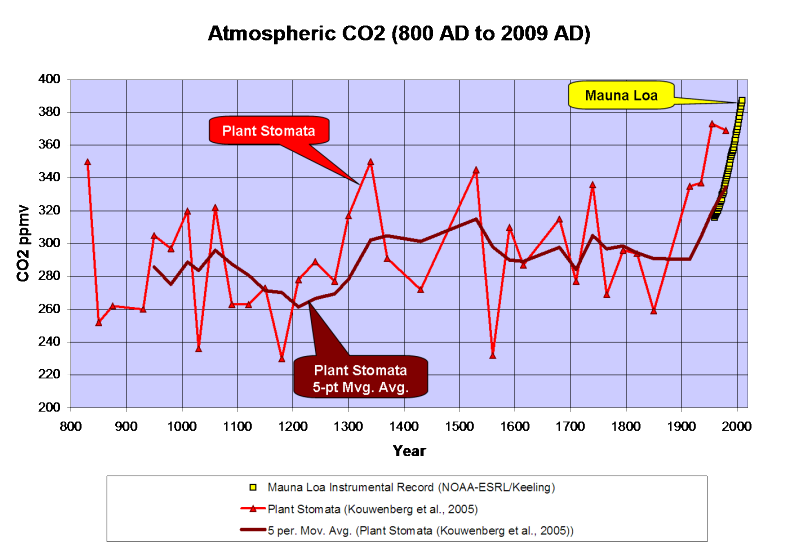
Kouwenberg et al., 2005 found that a “stomatal frequency record based on buried Tsuga heterophylla needles reveals significant centennial-scale atmospheric CO2 fluctuations during the last millennium.”
Plant stomata data show much greater variability of atmospheric CO2 over the last 1,000 years than the ice cores and that CO2 levels have often been between 300 and 340ppmv over the last millennium, including a 120ppmv rise from the late 12th Century through the mid 14th Century. The stomata data also indicate higher CO2 levels than the Mauna Loa instrumental record; but a 5-point moving average ties into the instrumental record quite nicely…

A survey of historical chemical analyses (Beck, 2007) shows even more variability in atmospheric CO2 levels than the plant stomata data since 1800…

WHAT DOES IT ALL MEAN?
The current “paradigm” says that atmospheric CO2 has risen from ~275ppmv to 388ppmv since the mid-1800’s as the result of fossil fuel combustion by humans. Increasing CO2 levels are supposedly warming the planet…

However, if we use Moberg’s (2005) non-Hockey Stick reconstruction, the correlation between CO2 and temperature changes a bit…

Moberg did a far better job in honoring the low frequency components of the climate signal. Reconstructions like these indicate a far more variable climate over the last 2,000 years than the “Hockey Sticks” do. Moberg also shows that the warm up from the Little Ice Age began in 1600, 260 years before CO2 levels started to rise.
As can be seen below, geologically consistent reconstructions like Moberg and Esper are in far better agreement with “direct” paleotemperature measurements, like Alley’s ice core reconstruction for Central Greenland…

In fairness to Dr. Mann, his 2008 reconstruction did restore the Medieval Warm Period and Little Ice Age to their proper places; but he still used Mike’s Nature Trick to slap a hockey stick blade onto the 20th century.
What happens if we use the plant stomata-derived CO2 instead of the ice core data?

We find that the ~250-year lag time is consistent. CO2 levels peaked 250 years after the Medieval Warm Period peaked and the Little Ice Age cooling began and CO2 bottomed out 240 years after the trough of the Little Ice Age. In a fashion similar to the glacial/interglacial lags in the ice cores, the plant stomata data indicate that CO2 has lagged behind temperature changes by about 250 years over the last millennium. The rise in CO2 that began in 1860 is most likely the result of warming oceans degassing.
While we don’t have a continuous stomata record over the Holocene, it does appear that a lag time was also present in the early Holocene…

Once dissolved in the deep-ocean, the residence time for carbon atoms can be more than 500 years. So, a 150- to 200-year lag time between the ~1,500-year climate cycle and oceanic CO2 degassing should come as little surprise.
CONCLUSIONS
-
Ice core data provide a low-frequency estimate of atmospheric CO2 variations of the glacial/interglacial cycles of the Pleistocene. However, the ice cores seriously underestimate the variability of interglacial CO2 levels.
-
GEOCARB shows that ice cores underestimate the long-term average Pleistocene CO2 level by 36ppmv.
-
Modern satellite data show that atmospheric CO2 levels in Antarctica are 20 to 30ppmv less than lower latitudes.
-
Plant stomata data show that ice cores do not resolve past decadal and century scale CO2 variations that were of comparable amplitude and frequency to the rise since 1860.
Thus it is concluded that:
-
CO2 levels from the Early Holocene through pre-industrial times were highly variable and not stable as the Antarctic ice cores suggest.
-
The carbon and climate cycles are coupled in a consistent manner from the Early Holocene to the present day.
-
The carbon cycle lags behind the climate cycle and thus does not drive the climate cycle.
-
The lag time is consistent with the hypothesis of a temperature-driven carbon cycle.
-
The anthropogenic contribution to the carbon cycle since 1860 is minimal and inconsequential.
Note: Unless otherwise indicated, all of the climate reconstructions used in this article are for the Northern Hemisphere.
References
Anklin, M., J. Schwander, B. Stauffer, J. Tschumi, A. Fuchs, J.M. Barnola, and D. Raynaud, CO2 record between 40 and 8 kyr BP from the GRIP ice core, Journal of Geophysical Research, 102 (C12), 26539-26545, 1997.
Wagner et al., 1999. Century-Scale Shifts in Early Holocene Atmospheric CO2 Concentration. Science 18 June 1999: Vol. 284. no. 5422, pp. 1971 – 1973.
Berner et al., 2001. GEOCARB III: A REVISED MODEL OF ATMOSPHERIC CO2 OVER PHANEROZOIC TIME. American Journal of Science, Vol. 301, February, 2001, P. 182–204.
Kouwenberg, 2004. APPLICATION OF CONIFER NEEDLES IN THE RECONSTRUCTION OF HOLOCENE CO2 LEVELS. PhD Thesis. Laboratory of Palaeobotany and Palynology, University of Utrecht.
Wagner et al., 2004. Reproducibility of Holocene atmospheric CO2 records based on stomatal frequency. Quaternary Science Reviews 23 (2004) 1947–1954.
Esper et al., 2005. Climate: past ranges and future changes. Quaternary Science Reviews 24 (2005) 2164–2166.
Kouwenberg et al., 2005. Atmospheric CO2 fluctuations during the last millennium reconstructed by stomatal frequency analysis of Tsuga heterophylla needles. GEOLOGY, January 2005.
Van Hoof et al., 2005. Atmospheric CO2 during the 13th century AD: reconciliation of data from ice core measurements and stomatal frequency analysis. Tellus (2005), 57B, 351–355.
Rundgren et al., 2005. Last interglacial atmospheric CO2 changes from stomatal index data and their relation to climate variations. Global and Planetary Change 49 (2005) 47–62.
Jessen et al., 2005. Abrupt climatic changes and an unstable transition into a late Holocene Thermal Decline: a multiproxy lacustrine record from southern Sweden. J. Quaternary Sci., Vol. 20(4) 349–362 (2005).
Beck, 2007. 180 Years of Atmospheric CO2 Gas Analysis by Chemical Methods. ENERGY & ENVIRONMENT. VOLUME 18 No. 2 2007.
Loulergue et al., 2007. New constraints on the gas age-ice age difference along the EPICA ice cores, 0–50 kyr. Clim. Past, 3, 527–540, 2007.
DATA SOURCES
CO2
Etheridge et al., 1998. Historical CO2 record derived from a spline fit (75 year cutoff) of the Law Dome DSS, DE08, and DE08-2 ice cores.
NOAA-ESRL / Keeling.
Berner, R.A. and Z. Kothavala, 2001. GEOCARB III: A Revised Model of Atmospheric CO2 over Phanerozoic Time, IGBP PAGES/World Data Center for Paleoclimatology Data Contribution Series # 2002-051. NOAA/NGDC Paleoclimatology Program, Boulder CO, USA.
Kouwenberg et al., 2005. Atmospheric CO2 fluctuations during the last millennium reconstructed by stomatal frequency analysis of Tsuga heterophylla needles. GEOLOGY, January 2005.
Lüthi, D., M. Le Floch, B. Bereiter, T. Blunier, J.-M. Barnola, U. Siegenthaler, D. Raynaud, J. Jouzel, H. Fischer, K. Kawamura, and T.F. Stocker. 2008. High-resolution carbon dioxide concentration record 650,000-800,000 years before present. Nature, Vol. 453, pp. 379-382, 15 May 2008. doi:10.1038/nature06949.
Royer, D.L. 2006. CO2-forced climate thresholds during the Phanerozoic. Geochimica et Cosmochimica Acta, Vol. 70, pp. 5665-5675. doi:10.1016/j.gca.2005.11.031.
TEMPERATURE RECONSTRUCTIONS
Moberg, A., et al. 2005. 2,000-Year Northern Hemisphere Temperature Reconstruction. IGBP PAGES/World Data Center for Paleoclimatology Data Contribution Series # 2005-019. NOAA/NGDC Paleoclimatology Program, Boulder CO, USA.
Esper, J., et al., 2003, Northern Hemisphere Extratropical Temperature Reconstruction, IGBP PAGES/World Data Center for Paleoclimatology Data Contribution Series # 2003-036. NOAA/NGDC Paleoclimatology Program, Boulder CO, USA.
Mann, M.E. and P.D. Jones, 2003, 2,000 Year Hemispheric Multi-proxy Temperature Reconstructions, IGBP PAGES/World Data Center for Paleoclimatology Data Contribution Series #2003-051. NOAA/NGDC Paleoclimatology Program, Boulder CO, USA.
Alley, R.B.. 2004. GISP2 Ice Core Temperature and Accumulation Data. IGBP PAGES/World Data Center for Paleoclimatology Data Contribution Series #2004-013. NOAA/NGDC Paleoclimatology Program, Boulder CO, USA.
VEIZER d18O% ISOTOPE DATA. 2004 Update.
P. Solar says:
December 30, 2010 at 12:49 am
Interesting accumulation of data but this is meaningless without showing the associated uncertainties.
Ice cores tell us nothing about the changes on a timescale comparable to the industrial period.
The available data is not able to prove or disprove that this is in anyway different or “unprecedented”. The whole discussion is totally without foundation.
Please, before writing such things, have a look at the existing data! The data of many ice cores are available at:
http://www.ncdc.noaa.gov/paleo/icecore/current.html
There are data from ice cores with very high accumulation (1.2 meter ice equivalent per year) like Law Dome and very low accumulation (a few mm per year) like Vostok and Dome C. The highest accumulation ice cores have a resolution of about a decade and span some 150 years. Some others have a 40 years resolution and go back 1,000 years and Dome C has a resolution of 560 years but goes back some 800,000 years.
For the past 1,000 years, that gives the following combination of datapoints from different ice cores with available points:
http://www.ferdinand-engelbeen.be/klimaat/klim_img/antarctic_cores_001kyr.jpg
While the accumulation rate and temperature and salt/dust inclusions are quite different for the different cores, the CO2 levels found are quite identical for the same gas age (+/- 5 ppmv). The highest accumulation cores of Law Dome (with an accuracy of +/- 1.2 ppmv – 1 sigma) even have an overlap of some 20 years with direct measurements of the South Pole:
http://www.ferdinand-engelbeen.be/klimaat/klim_img/law_dome_sp_co2.jpg
Thus while Mann’s HS was certainly fabricated, the CO2 HS is quite real, at least for the past 10,000 years and probably 800,000 years: one need quite rapid and large changes of temperature to induce rapid and large changes of CO2… The CO2 : temperature ratio in the long run was about 8 ppmv/°C. To obtain a 100 ppmv increase in 150 years by natural causes, one need an increase of 12°C in the same time span. Not completely unprecedented (the end of the Younger Dryas), but quite uncommon and not global. And not lasting for long: even the 560 years resolution of Dome C would notice a 100 ppmv increase lasting over a 20 years time span.
David Middleton says:
December 29, 2010 at 6:36 am
Your question does beg the converse questions… “How much of the lower variability in the Antarctic ice cores is due to the lower resolution due to the low snow accumulation rates? How much of the lower variability is due to the relative meteorological isolation of Antarctica? How much of the lower variability is due to the effects of burial compaction?”
Burial compaction makes that the layers are smaller with depth and thus the resolution get worse.
Then the resolution goes down together with the accumulation rate, but is sufficient over the past 1,000 years to show the influence of the MWP-LIA difference on CO2 levels (about 6 ppmv for an about 0.8°C temperature difference) in a few ice cores. The isolation of Antarctica for CO2 is that the whole SH lags the NH with about one year, which shows that the main source of extra CO2 is in the NH. And the SH has less influence of the seasonal variations (which are caused by vegetation growth and decay). That doesn’t play much role for the averaging of the ice cores, which is about a decade for the fastest accumulating ones. In contrast, CO2 levels over land have a positive bias and are highly variable, even if they show a similar trend as the South Pole data (and thus the ice core data). Here the monthly averages of Giessen (a few hundred km SW of one of the main places where stomata data were taken over the past millennium in The Netherlands)
http://www.ferdinand-engelbeen.be/klimaat/klim_img/giessen_mlo_monthly.jpg
here compared to the (“cleaned”) Mauna Loa monthly averages, the South Pole data are less seasonably influenced and some 3 ppmv below the MLO data with a similar trend.
I am pretty sure that the CO2 variability at St. Odiliënberg (where the stomata data were taken) is as high as in Giessen. Reason why I think that any CO2 data taken over land, be it directly (historical, wet methods) or indirectly (via stomata) must be taken with some grains (or a lot of) salt…
Here a few days in summer of the raw (!) CO2 data from Giessen, Barrow (Alaska), Mauna Loa and the South Pole at full scale:
http://www.ferdinand-engelbeen.be/klimaat/klim_img/giessen_background_zero.jpg
Thus in how far the variability seen in the stomata data is reflecting “global” changes of CO2 remains an open question for me.
Ferdinand,
The last sentence of your most recent comment is the perfect example of a scientific thought process…
In science, most questions should remain open.
As always, thank you for the very constructive input.
Ferdinand Engelbeen says:
December 30, 2010 at 5:09 pm
Here a few days in summer of the raw (!) CO2 data from Giessen, Barrow (Alaska), Mauna Loa and the South Pole at full scale:
http://www.ferdinand-engelbeen.be/klimaat/klim_img/giessen_background_zero.jpg
Hi Ferdinand,
Do you have a plot of seasonal variation at Giessen?
Thanks
tallbloke says:
December 31, 2010 at 4:05 am
Hi Ferdinand,
Do you have a plot of seasonal variation at Giessen?
Should be visible in the monthly averages, but is hardly detectable in the huge noise over more than a decade of data:
http://www.ferdinand-engelbeen.be/klimaat/klim_img/giessen_mlo_monthly.jpg
I have no idea what caused the few extreme peaks in the Giessen data, but in general CO2 levels taken over land are very noisy and influenced by crops, industry, traffic, heating,… and what/how much of these sinks and sources are present in the main wind direction of that particular month. Or growing season for stomata data: according to Dr. Tom Van Hoof, stomata density of new leaves is based on CO2 levels in the previous growing season.
Here another plot of land based monthly CO2 averages near Kennedy Space Centre (Florida, USA), compared to several “baseline” stations over a few years:
http://www.ferdinand-engelbeen.be/klimaat/klim_img/month_2002_2006_ken.jpg
Again hardly any seasonal variation detectable in the huge noise…
The Kennedy Space Center Scrub Oak site is located within the Merritt Island National Wildlife Refuge at the Kennedy Space Center (KSC) on the east coast of central Florida, within a 10 ha park. See:
http://public.ornl.gov/ameriflux/Site_Info/siteInfo.cfm?KEYID=us.ksc_scruboak.01
That is part of the Ameriflux network, aimed to obtain more details about the back and forth fluxes of CO2 over vegetation (and human sources) over the seasons. Not an easy task… See more details at:
http://public.ornl.gov/ameriflux/dataproducts.shtml
Pieter Tans of NOAA has a few plots of the Wisconsin tall tower of summer/winter CO2 taken at different heights at:
http://www.esrl.noaa.gov/gmd/ccgg/about/co2_measurements.html
Ferdinand Engelbeen, I understand it’s hard to wade thru all these comments, so I’ll ask again.
How does the time-lag of CO2 diffusion affect the apparent time-lags of CO2 vs temp? It’s been assumed to be ~800 yrs at the interglacial start and ~1200 yrs at the beginning of the glacial period. Or is the data not detailed enough to determine this?
I looked at your site & couldn’t find anything about this directly.
beng says:
December 31, 2010 at 5:29 am
Ferdinand Engelbeen, I understand it’s hard to wade thru all these comments, so I’ll ask again.
How does the time-lag of CO2 diffusion affect the apparent time-lags of CO2 vs temp? It’s been assumed to be ~800 yrs at the interglacial start and ~1200 yrs at the beginning of the glacial period. Or is the data not detailed enough to determine this?
I looked at your site & couldn’t find anything about this directly.
Indeed, I am just half way the comments now…
The main problem of the diffusion for low accumulation cores is to determine the average age of the air in the gas bubbles and the averaging period that the air represents. The main way is by firn densification models, which were validated by direct measurements of the CO2 levels in open pores of the firn top-down.
An additional problem is that during the cold glacial periods, the accumulation (and thus the firm densification) is even less than during an interglacial.
For some periods, there is some help from known volcanic eruptions (dust, sulfate deposits) and comparisons with ocean sediments and overlapping periods in other ice cores (Antarctic and Greenland). And changes in isotopic composition of the different gases are used to determine the timing of land changes from ice covered to vegetation covered and back.
Nevertheless, there are several corrections issued for different ice cores, where better methods of analyses show (small to important) changes in gas age timing. That is less of a problem for the determination of the age if the ice layers, where the d18O and dD ratio’s gives a quite good information of nearby (for coastal ice cores) to hemispheric (for the inland ice cores) ocean temperatures.
Thus the timing of the changes in the gas composition vs. the temperature (proxies) remains problematic, the more that the resolution of the Vostok ice core is around 600 years. One can only be sure that there is a lag, but less sure if that is small or huge.
For the last end of the glacial period, there are more data from a higher sampling density at Dome C: the resolution still is around 560 years, but samples were taken on small parts of the ice, allowing for more datapoints (about 6 per millenium). That gives a somewhat better insight in the variability of the lag, but in absolute value to be taken with a grain of salt:
http://www.ferdinand-engelbeen.be/klimaat/klim_img/epica5.gif
The graph was made by André van den Berg, based on the Dome C data.
Some more literature:
http://www.sciencemag.org/content/283/5408/1712.abstract
http://www.ncdc.noaa.gov/paleo/taylor/indermuehle00grl.pdf
The latter looked at the D.-O. events and found a lag of 1200 +/- 700 years by a Monte Carlo analyses for a best fit of the temperature-CO2 correlation.
G.L. Alston says:
December 27, 2010 at 5:37 am
1. We’re constantly told that the rise from 1800 onward (that’s 200+ years) is anthropogenic. CO2 is up. Temps must therefore rise. It’s so well known that this results in the skeptics reminding all that correlation isn’t causation.
2. Advocates tell us there’s a relationship between temp and CO2. To explain ice core lags (or handwave or whatever) the idea is that if temp goes up CO2 will go up, PERIOD. There is no uptick in temp without an uptick in CO2, and it doesn’t matter which one drive which — there’s a correlation. When one goes up, the other one does.
1. Is right: humans are responsible for (most of) the 100+ ppmv rise of CO2 levels in the past 150 years. There is a lot of evidence for that and none of the observations are contrary this evidence. Any alternative explanation fails one or more observations.
2. Is questionable. Even without any rise of CO2, temperature is leading the way. But GCM’s imply a huge feedback from CO2, as these overlap over a long period during glacial-interglacial transitions. But other feedbacks may have been underestimated (clouds, albedo), rendering CO2 feedback to an absolute minimum, as can be seen in the long lags of CO2 during the opposite transition:
http://www.ferdinand-engelbeen.be/klimaat/eemian.html
The fact that A causes B doesn’t exclude that B may have an influence on A. As long as the combined factor not is greater than 1, there is no runaway process. In the case of temperature and CO2, CO2 responds with about 8 ppmv/°C over the ice ages and the MWP-LIA difference (and currently with 4 ppmv/°C for short term variability around the trend). Opposite, the (lab measured) response of temperature to 2xCO2 is about 0.9°C. In how far other processes like water vapour, cloud feedback etc… on this water planet, increase or decrease the temperature is still an open question…
David Middleton says:
December 27, 2010 at 1:01 pm
Knorr, 2009 showed that about 60% of the annual anthropogenic emissions are taken up by sinks. The sinks can’t tell the difference between this year’s and last year’s CO2 emissions. It’s a roughly 60% decay rate. This fits the well-established residence time of 5 to 15 years (Essenhigh, 2009, Segalstad, 1998, Segalstad, 1982, Houghton et al., 1990, Stumm & Morgan, 1970, Revelle & Suess, 1957, etc.).
David, like so many before you, you are confusing residence time (which is how much CO2 is exchanged between the different reservoirs each year) with excess CO2 decay time. The former is about 150 GtC/800 GtC present in the atmosphere. That doesn’t change the total amount of CO2 in the atmosphere with one gram. The excess decay rate is what matters: 60% of the emissions (including land use changes) is only 5 GtC/year real reduction of the total amount of CO2 emitted (some 9 GtC/year), thus the real excess decay rate is about 40 years half life time if we should stop all emissions today. Not 5-15 years. And as the difference still is 4 GtC/year, that is what shows up as extra increase in the atmosphere, whatever the origin of the molecules of CO2 which were captured or released by the CO2 exchanges with other reservoirs.
Joel Shore says:
December 28, 2010 at 6:05 pm
“If you are really think that you can fit a quadratic over only 2 or 4 years of the data and draw a serious conclusion then you deserve whatever answer you get!”
It’s two decades, Buckaroo. The curve fit is over two decades, and it is a smooth and typically natural function of time. You recognize these things when you’ve been at it as long as I.
Ferdinand Engelbeen says:
December 30, 2010 at 3:53 pm
“Well you are completely wrong on this.”
Oh, Ferdinand… I’ve tried, but I cannot explain it to you. This just isn’t your area of expertise. All of the information needed has been covered above. You are simply wrong.
Stephen Rasey says:
December 27, 2010 at 11:40 pm
At first glance, it might seem that the trapped air may be richer in CO2 than in the atmosphere at deposition because the CO2 molecule is larger and heavier than N2 and O2. But with a variable pressure and diurnal temperature, as that constricting bubble breathes, once a CO2 escapes, it is much less likely to reenter than an O2 or N2.
The other point I did not see mentioned here is the relative solubility of the air gases in Ice and water. When dealing with ppm’s, is the solubility of CO2 on the surface of an ice crystal inconsequential?
Indeed there is some fractionation of the heavier molecules and isotopes in the lower firn layers. This is compensated for by taking into account the fractionation of 15N/14N with depth. See:
http://www.pnas.org/content/94/16/8343.full
Further, the smallest molecules (Ne, Ar, O2) show a deficit in the resultant air bubbles, because these may still escape during the closing process below a certain porosity. The vibrational diameter of CO2 is somewhat above this porosity diameter, thus doesn’t show such a deficit. See:
http://icebubbles.ucsd.edu/Publications/closeoff_EPSL.pdf
Water is less of a problem, as the waterlike layer at the ice – air surface is about 5 atoms thick and even less waterlike at the intercrystalline borders. Migration of CO2 is extremely low, even for the higher temperature (-20°C) ice cores. And any CO2 dissolved in some water is effectively removed as the measurements are made under vacuum, removing any water over a cold trap and destructing any remaining clathrates. Comparison of this method with another method, where all ice is sublimated and cryogenically separated (mostly done for more accurate mass spectrometer analyses of isotopes) shows the same results…
Enough for today and this year…
Hope you may all enjoy a New Year in good health and lots of discussions…
Happy New Year!
Ferdinand
Joel Shore says:
December 26, 2010 at 7:33 pm
“Exactly! Why is it not obvious to all scientists that CO2 levels before 1959 danced around wildly before 1960, but in a very careful choreographed manner so that the level remained within about 10ppm when effectively low-pass filtered in the ice core data?”
Aye, yi, yi. I just saw this comment. Joel might as well have just broadcast “I know nothing about filtering theory or how ARMA processes work.” Because, that is what this statement reveals. This is precisely what a low pass filter does. It’s not magic. It’s math. It’s what is done every single day in real time as you tune a radio or TV station, or make a call on your cell phone.
Ferdinand Engelbeen says:
December 31, 2010 at 1:34 pm
When, oh when, will you learn the difference between conjecture and proven facts? Maybe in the new year? This is so depressing…
Bart says:
December 31, 2010 at 12:58 pm
Oh, Ferdinand… I’ve tried, but I cannot explain it to you. This just isn’t your area of expertise. All of the information needed has been covered above. You are simply wrong.
Try somewhat harder. My area of (past) expertise is process (automation) engineering, but already 7 years retired…
What you are doing is looking at the derivative of the trend: the year by year emissions, and compare that to the year by year increase in the atmosphere. Thus you are looking at the cause of the noise around the trend, not the trend itself. That noise is mainly caused by year by year temperature variations which influence the uptake of CO2 by oceans and vegetation. That is agreed by “coolers” and “warmers” alike, see the paper by Pieter Tans for the 50 years Mauna Loa festivities:
http://esrl.noaa.gov/gmd/co2conference/pdfs/tans.pdf
His conclusion:
Conclusion:
2/3 of the interannual variance of the CO2 growth rate is explained by the delayed response of the terrestrial biosphere to interannual variations of temperature and precipitation.
Even so, the emissions are about twice the increase in the atmosphere, thus anyone with a minimum sense of logic can tell you that whatever the rest of nature does, the increase in the atmosphere is caused by the emissions, as nature as a whole is a net sink for CO2. Whatever the individual natural flows might be or however these changed over time. At least for the past 50 years of accurate measurements and probably for the past 100+ years. That is what the mass balance tells us.
As no carbon is escaping to space, as long as the increase in the atmosphere is less than the emissions, there is no net contribution of nature. Nothing, nada, zero.
Here a comparison of the accumulation in the atmosphere and the accumulated emissions over the past decades of accurate measurements:
http://www.ferdinand-engelbeen.be/klimaat/klim_img/acc_co2_1960_2006.jpg
If you have any proof that one can have an increase in the atmosphere less than the emissions, and “something else” may be the cause of the increase, you may be a candidate for the Nobel Price of physics by the creation of matter from nothing and/or the destruction of matter to nothing…
Bart says:
December 31, 2010 at 8:22 pm
When, oh when, will you learn the difference between conjecture and proven facts? Maybe in the new year? This is so depressing…
Sometimes it helps if you read the existing literature…
The migration of CO2 in ice cores was theoretically calculated by looking at the migration in remelted layers of a “warm” (-24°C) ice core, Siple Dome:
http://catalogue.nla.gov.au/Record/3773250
The extra smoothing of the gas age averaging caused by migration is about 2 orders of magnitude less than the averaging itself. For the Siple Dome ice core, the average gas resolution is about 22 years. Migration increases that with about 0.2 years.
At lowest depth, the layers become thinner and migration may relatively increase and give a doubling of the resolution to some 40 years.
The Vostok and Dome C ice cores are much older at depth, but also much colder (-40°C), which means less water (no water layer at all at -32°C, as long as no salt inclusions are involved). But there is a simple proof that migration doesn’t play a role at Vostok and Dome C:
The Vostok (and Dome C) ice cores show a quite nice relationship between the temperature proxy (dD and d18O) and CO2 levels, be it with a lag. Nevertheless, the ratio between CO2 and temperature is about 8 ppmv/°C between interglacials and glacial periods over the past 420,000 years (recently conformed for the full 800,000 years in Dome C). If there was some migration, the ratio would fade over time for each 100,000 years period further back. That is not the case. Thus there is little migration of CO2 in the Vostok and Dome C ice cores…
David Middleton says:
December 27, 2010 at 7:34 am
Some more comment on:
Mankind puts 6 to 8 GtC worth of CO2 into the atmosphere every year. Plant respiration accounts for 40 to 50 GtC, residuum decay accounts for 50 to 60 GtC and sea-surface gas exchanges accounts for 100 to 115 GtC. The total range of natural sources is 190 to 235 GtC. Anthropogenic emissions are less than 1/5 of the annual variability of the natural sources. Furthermore, ~60% of the annual anthropogenic emissions are taken up by sinks.
There are natural sources and natural sinks. While human emissions are currently about 8 GtC/year, the variability of all natural sinks and sources together is less than +/- 5 GtC (2.5 ppmv) globally over the seasons and less than +/- 2 GtC (1 ppmv) in year to year variability. Main reason for the relative small natural variability is that a temperature increase/decrease works countercurrent for vegetation and ocean uptake (warmer means less CO2 uptake by the oceans and more CO2 uptake by vegetation):
http://www.ferdinand-engelbeen.be/klimaat/klim_img/dco2_em.jpg
Thus human emissions are about twice the seasonal variability and 4 times the year by year variability, whatever the individual natural flows within a year might be.
Further, while 60% of the emissions in total mass are absorbed, that isn’t caused by the one-year emissions, but by the total difference of pCO2 in the atmosphere and the pCO2 of the oceans (and similar in the plant alveoles). Thus it is the change in total atmospheric CO2 which makes that the oceans and vegetation are increasing in uptake, modulated by temperature variations. That the uptake is increasing at a near fixed rate with the emissions, probably is the result of ever increasing emissions, slightly exponential.
The behaviour of the CO2 carbon cycle looks like a simple first order physical process: as long as the emissions are increasing, the increase in the atmosphere follows at a more or less fixed rate…
Bart says:
A low-pass filter would only work this way if all of the frequencies in the signal (with sufficient amplitude) were much greater than the cutoff frequency of the filter. This would seem highly unlikely on the face of it but now that we have about 50 years of steadily-rising data from Mauna Loa, I think we can say with confidence that there is already a low enough frequency in that data that this statement cannot be true (at least for the faster accumulating ice cores). [I haven’t tried fitting sine curves to the Mauna Loa data but I imagine that if you did then you would be hard-pressed to get this 50 years as even representing a quarter of a cycle, which means that the period would be at least 200 years.]
Ferdinand Engelbeen says:
January 1, 2011 at 2:04 am
“Thus you are looking at the cause of the noise around the trend, not the trend itself.”
No. It is a consistent, decades long, coherent signal. It is not noise.
Ferdinand Engelbeen says:
January 1, 2011 at 2:31 am
“Sometimes it helps if you read the existing literature…”
Sometimes, it helps to think for yourself, and question what you are being spoon fed without sufficient evidence.
Joel Shore says:
January 1, 2011 at 8:10 am
“I think we can say with confidence…”
What do you mean “we”, paleface? We’re not talking about Mauna Loa data here. We are talking about what the ice core data show over time. And, you won’t know for hundreds of years what it will record for the current era.
Ferdinand Engelbeen says:
January 1, 2011 at 2:04 am
“That is what the mass balance tells us.”
It really doesn’t tell us that at all, Ferdinand. I do not know why you cannot grasp your fallacy here. I only know that you cannot, because we have been over and over it, and others have tried to explain it to you, too. It is painful to watch.
Bart says:
January 1, 2011 at 10:05 am
Sometimes, it helps to think for yourself, and question what you are being spoon fed without sufficient evidence.
Bart,
I see that it is to no avail to have a further discussion about these topics. If you don’t think that the available literature has at least something that may be true (even if that doesn’t fit your ideas), then we can’t have any further discussion on that topic.
And I have a nice habit to think for myself, no matter what is said by others (at both sides of the warmist/cooler camps). Only that I accept what is said by others if it seems reasonable, even if it is against my own ideas.
About thinking for yourself: can you explain why there is no fading away of the CO2:temperature ratio over 800,000 years time if there was even the slightest migration of CO2 through the ice?
Ferdinand Engelbeen – First of all, many thanks for your many contributions to WUWT. To my mind, you are dealing with everything in a truly scientific manner, addressing the facts in an open and professional way, putting all your arguments into the open for everyone to see and to test. When people disagree with you (as I have in the past, and may do in the future) you patiently deal with the science itself. If those who promote AGW had taken the same approach as you, we would have far fewer problems.
I see that you are still saying “Even so, the emissions are about twice the increase in the atmosphere, thus anyone with a minimum sense of logic can tell you that whatever the rest of nature does, the increase in the atmosphere is caused by the emissions, as nature as a whole is a net sink for CO2. Whatever the individual natural flows might be or however these changed over time.“.
Mathematically, simple logic does not tell you that the increase in the atmosphere is caused by the emissions. It tells you only that without the emissions, the increase would have been less by an unspecified amount which could have been large (0%).
However, in the real world, where CO2 transfers between ocean and atmosphere are driven by physical laws (including but not limited to Henry’s Law), and where past temperature and CO2 data give us additional clues, it is clear that the amount of atmospheric CO2 increase absent emissions would have been nearer to 0% than 100% of the observed increase. From previous discussions between us on this subject on WUWT, and using the ice core data as the main guide to the temperature/CO2 behaviour, it appears that CO2 would have risen naturally by something like 6-12% of the observed rise, but the figures are unreliable because we are talking about the rise over a few decades while ice cores have a resolution typically in 100’s of years. (Plant stomata and other data indicate that CO2 may vary more over decadal periods than the ice core data indicates). But you have now said “…humans are responsible for (most of) the 100+ ppmv rise of CO2 levels in the past 150 years. There is a lot of evidence for that and none of the observations are contrary this evidence. Any alternative explanation fails one or more observations.” [my emphasis] all of which I agree with, and which I will take as putting the argument to rest.
Bart – “[Humans are not the reason why CO2 keeps creeping up]. The increase in CO2 concentration bears only a superficial resemblance to the human production of CO2. The two series correlate poorly in the low frequency regime, and not to any level of significance at all in the higher frequency realm.“.
I too have put a lot of [amateur] work into analysing CO2 variations and temperature. Whereas you have apparently concentrated on the “charts”, I also tried to look at the possible physical processes. The correlation between temperature and annual CO2 changes looks compelling, but I am satisfied that it gives a short term variation operating on a longer term trend , and the principal obvious cause of the trend is human-emitted CO2. That doesn’t prove that human-emitted CO2 is the only cause, or even the main cause, but Occham’s razor says that in the absence of data showing otherwise we should accept [at least provisionally] that human-emitted CO2 is the cause.
Bart – “we could be experiencing an upwelling of CO2 sequestered long ago giving a strong signal“.
I looked at this possibility too. Using the given figures for ocean circulation, and the highest deep-ocean CO2 concentrations that I thought likely, I could not get an upwelling of CO2 large enough to give the observed CO2 increase.
Nothing I have done actually proves anything of course, and as in all science everything is provisional.
Bart – one last comment: However frustrated you may get, the “Engelbeen model” of civility is worth following. Even Joel Shore, who often gets given a pretty hard time on WUWT, generally (always?) sticks to the science.
Correction : I used some “less than” and “greater than” signs in the text which must have got translated as html. For “an unspecified amount which could have been large (0%).” read “an unspecified amount which could have been large (less than 100%) or tiny (greater than 0%).“
Bart says:
January 1, 2011 at 10:05 am
“Thus you are looking at the cause of the noise around the trend, not the trend itself.”
No. It is a consistent, decades long, coherent signal. It is not noise.
I am not sure where you are talking about. The trend of accumulation of the emissions and the trend of accumulation in the atmosphere show an incredible good correlation. While correlation is not proof of causation, I don’t think that in this case the increase in the atmosphere caused the emissions. Or that any natural cause can show such a perfect match over time with the emissions. Not only over the MLO period, but even so back to 1900, based on ice cores with a resolution of about a decade.
If you only look at the year by year emissions and increase in the atmosphere, you are looking at the first derivative of the trend, not the trend itself, which is influenced by (at least) two variables: the emissions and the variability in sink rate, which is mainly influenced by the temperature variability, but the latter is less important for changes over the past century, as the temperature only shows a small change over the total period.
Mike Jonas says:
January 1, 2011 at 1:16 pm
Thanks for your kind words! I think that we do agree on most of what you said…
Bart says:
January 1, 2011 at 10:19 am
It really doesn’t tell us that at all, Ferdinand. I do not know why you cannot grasp your fallacy here. I only know that you cannot, because we have been over and over it, and others have tried to explain it to you, too. It is painful to watch.
I still wonder why so many brilliant persons have such a problem with the basic logic of a mass balance, while most housewives know that from their own budget:
If you add 100 euro’s (dollars,…) every morning in your wallet and end the day with 50 dollar more than at the end of the previous day and you repeat that for weeks, then the increase of money in your wallet is entirely caused by the daily addition of 100 euro’s. No matter how much ins and outs you had of your wallet over the rest of the day. The housewive knows that, besides the daily addition, the rest of the day there was a net expense of 50 euro’s, so there was no net gain from “something else”.