Guest post by David Middleton
INTRODUCTION
Anyone who has spent any amount of time reviewing climate science literature has probably seen variations of the following chart…

A record of atmospheric CO2 over the last 1,000 years constructed from Antarctic ice cores and the modern instrumental data from the Mauna Loa Observatory suggest that the pre-industrial atmospheric CO2 concentration was a relatively stable ~275ppmv up until the mid 19th Century. Since then, CO2 levels have been climbing rapidly to levels that are often described as unprecedented in the last several hundred thousand to several million years.
Ice core CO2 data are great. Ice cores can yield continuous CO2 records from as far back as 800,000 years ago right on up to the 1970’s. The ice cores also form one of the pillars of Warmista Junk Science: A stable pre-industrial atmospheric CO2 level of ~275 ppmv. The Antarctic ice core-derived CO2 estimates are inconsistent with just about every other method of measuring pre-industrial CO2 levels.
Three common ways to estimate pre-industrial atmospheric CO2 concentrations (before instrumental records began in 1959) are:
1) Measuring CO2 content in air bubbles trapped in ice cores.
2) Measuring the density of stomata in plants.
3) GEOCARB (Berner et al., 1991, 1999, 2004): A geological model for the evolution of atmospheric CO2 over the Phanerozoic Eon. This model is derived from “geological, geochemical, biological, and climatological data.” The main drivers being tectonic activity, organic matter burial and continental rock weathering.
ICE CORES
The advantage of Antarctic ice cores is that they can provide a continuous record of relative CO2 changes going back in time 800,000 years, with a resolution ranging from annual in the shallow section to multi-decadal in the deeper section. Pleistocene-age ice core records seem to indicate a strong correlation between CO2 and temperature; although the delta-CO2 lags behind the delta-T by an average of 800 years… 
Ice cores from Greenland are rarely used in CO2 reconstructions. The maximum usable Greenland record only dates as far back as ~130,000 years ago (Eemian/Sangamonian); the deeper ice has been deformed. The Greenland ice cores do tend to have a higher resolution than the Antarctic cores because there is a higher snow accumulation rate in Greenland. Funny thing about the Greenland cores: They show much higher CO2 levels (330-350 ppmv) during Holocene warm periods and Pleistocene interstadials. The Dye 3 ice core shows an average CO2 level of 331 ppmv (+/-17) during the Preboreal Oscillation (~11,500 years ago). These higher CO2 levels have been explained away as being the result of in situ chemical reactions (Anklin et al., 1997).
PLANT STOMATA
Stomata are microscopic pores found in leaves and the stem epidermis of plants. They are used for gas exchange. The stomatal density in some C3 plants will vary inversely with the concentration of atmospheric CO2. Stomatal density can be empirically tested and calibrated to CO2 changes over the last 60 years in living plants. The advantage to the stomatal data is that the relationship of the Stomatal Index and atmospheric CO2 can be empirically demonstrated…

When stomata-derived CO2 (red) is compared to ice core-derived CO2 (blue), the stomata generally show much more variability in the atmospheric CO2 level and often show levels much higher than the ice cores…

Plant stomata suggest that the pre-industrial CO2 levels were commonly in the 360 to 390ppmv range.
GEOCARB
GEOCARB provides a continuous long-term record of atmospheric CO2 changes; but it is a very low-frequency record…

The lack of a long-term correlation between CO2 and temperature is very apparent when GEOCARB is compared to Veizer’s d18O-derived Phanerozoic temperature reconstruction. As can be seen in the figure above, plant stomata indicate a much greater range of CO2 variability; but are in general agreement with the lower frequency GEOCARB model.
DISCUSSION
Ice cores and GEOCARB provide continuous long-term records; while plant stomata records are discontinuous and limited to fossil stomata that can be accurately aged and calibrated to extant plant taxa. GEOCARB yields a very low frequency record, ice cores have better resolution and stomata can yield very high frequency data. Modern CO2 levels are unspectacular according to GEOCARB, unprecedented according to the ice cores and not anomalous according to plant stomata. So which method provides the most accurate reconstruction of past atmospheric CO2?
The problems with the ice core data are 1) the air-age vs. ice-age delta and 2) the effects of burial depth on gas concentrations.
The age of the layers of ice can be fairly easily and accurately determined. The age of the air trapped in the ice is not so easily or accurately determined. Currently the most common method for aging the air is through the use of “firn densification models” (FDM). Firn is more dense than snow; but less dense than ice. As the layers of snow and ice are buried, they are compressed into firn and then ice. The depth at which the pore space in the firn closes off and traps gas can vary greatly… So the delta between the age of the ice and the ago of the air can vary from as little as 30 years to more than 2,000 years.
The EPICA C core has a delta of over 2,000 years. The pores don’t close off until a depth of 99 m, where the ice is 2,424 years old. According to the firn densification model, last year’s air is trapped at that depth in ice that was deposited over 2,000 years ago.
I have a lot of doubts about the accuracy of the FDM method. I somehow doubt that the air at a depth of 99 meters is last year’s air. Gas doesn’t tend to migrate downward through sediment… Being less dense than rock and water, it migrates upward. That’s why oil and gas are almost always a lot older than the rock formations in which they are trapped. I do realize that the contemporaneous atmosphere will permeate down into the ice… But it seems to me that at depth, there would be a mixture of air permeating downward, in situ air, and older air that had migrated upward before the ice fully “lithified”.
A recent study (Van Hoof et al., 2005) demonstrated that the ice core CO2 data essentially represent a low-frequency, century to multi-century moving average of past atmospheric CO2 levels.

It appears that the ice core data represent a long-term, low-frequency moving average of the atmospheric CO2 concentration; while the stomata yield a high frequency component.
The stomata data routinely show that atmospheric CO2 levels were higher than the ice cores do. Plant stomata data from the previous interglacial (Eemian/Sangamonian) were higher than the ice cores indicate…

The GEOCARB data also suggest that ice core CO2 data are too low…

The average CO2 level of the Pleistocene ice cores is 36ppmv less than GEOCARB…

Recent satellite data (NASA AIRS) show that atmospheric CO2 levels in the polar regions are significantly less than in lower latitudes…


So… The ice core data should be yielding lower CO2 levels than the Mauna Loa Observatory and the plant stomata.
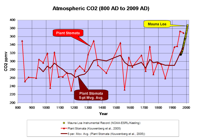
Kouwenberg et al., 2005 found that a “stomatal frequency record based on buried Tsuga heterophylla needles reveals significant centennial-scale atmospheric CO2 fluctuations during the last millennium.”
Plant stomata data show much greater variability of atmospheric CO2 over the last 1,000 years than the ice cores and that CO2 levels have often been between 300 and 340ppmv over the last millennium, including a 120ppmv rise from the late 12th Century through the mid 14th Century. The stomata data also indicate higher CO2 levels than the Mauna Loa instrumental record; but a 5-point moving average ties into the instrumental record quite nicely…

A survey of historical chemical analyses (Beck, 2007) shows even more variability in atmospheric CO2 levels than the plant stomata data since 1800…

WHAT DOES IT ALL MEAN?
The current “paradigm” says that atmospheric CO2 has risen from ~275ppmv to 388ppmv since the mid-1800’s as the result of fossil fuel combustion by humans. Increasing CO2 levels are supposedly warming the planet…

However, if we use Moberg’s (2005) non-Hockey Stick reconstruction, the correlation between CO2 and temperature changes a bit…

Moberg did a far better job in honoring the low frequency components of the climate signal. Reconstructions like these indicate a far more variable climate over the last 2,000 years than the “Hockey Sticks” do. Moberg also shows that the warm up from the Little Ice Age began in 1600, 260 years before CO2 levels started to rise.
As can be seen below, geologically consistent reconstructions like Moberg and Esper are in far better agreement with “direct” paleotemperature measurements, like Alley’s ice core reconstruction for Central Greenland…

In fairness to Dr. Mann, his 2008 reconstruction did restore the Medieval Warm Period and Little Ice Age to their proper places; but he still used Mike’s Nature Trick to slap a hockey stick blade onto the 20th century.
What happens if we use the plant stomata-derived CO2 instead of the ice core data?

We find that the ~250-year lag time is consistent. CO2 levels peaked 250 years after the Medieval Warm Period peaked and the Little Ice Age cooling began and CO2 bottomed out 240 years after the trough of the Little Ice Age. In a fashion similar to the glacial/interglacial lags in the ice cores, the plant stomata data indicate that CO2 has lagged behind temperature changes by about 250 years over the last millennium. The rise in CO2 that began in 1860 is most likely the result of warming oceans degassing.
While we don’t have a continuous stomata record over the Holocene, it does appear that a lag time was also present in the early Holocene…

Once dissolved in the deep-ocean, the residence time for carbon atoms can be more than 500 years. So, a 150- to 200-year lag time between the ~1,500-year climate cycle and oceanic CO2 degassing should come as little surprise.
CONCLUSIONS
-
Ice core data provide a low-frequency estimate of atmospheric CO2 variations of the glacial/interglacial cycles of the Pleistocene. However, the ice cores seriously underestimate the variability of interglacial CO2 levels.
-
GEOCARB shows that ice cores underestimate the long-term average Pleistocene CO2 level by 36ppmv.
-
Modern satellite data show that atmospheric CO2 levels in Antarctica are 20 to 30ppmv less than lower latitudes.
-
Plant stomata data show that ice cores do not resolve past decadal and century scale CO2 variations that were of comparable amplitude and frequency to the rise since 1860.
Thus it is concluded that:
-
CO2 levels from the Early Holocene through pre-industrial times were highly variable and not stable as the Antarctic ice cores suggest.
-
The carbon and climate cycles are coupled in a consistent manner from the Early Holocene to the present day.
-
The carbon cycle lags behind the climate cycle and thus does not drive the climate cycle.
-
The lag time is consistent with the hypothesis of a temperature-driven carbon cycle.
-
The anthropogenic contribution to the carbon cycle since 1860 is minimal and inconsequential.
Note: Unless otherwise indicated, all of the climate reconstructions used in this article are for the Northern Hemisphere.
References
Anklin, M., J. Schwander, B. Stauffer, J. Tschumi, A. Fuchs, J.M. Barnola, and D. Raynaud, CO2 record between 40 and 8 kyr BP from the GRIP ice core, Journal of Geophysical Research, 102 (C12), 26539-26545, 1997.
Wagner et al., 1999. Century-Scale Shifts in Early Holocene Atmospheric CO2 Concentration. Science 18 June 1999: Vol. 284. no. 5422, pp. 1971 – 1973.
Berner et al., 2001. GEOCARB III: A REVISED MODEL OF ATMOSPHERIC CO2 OVER PHANEROZOIC TIME. American Journal of Science, Vol. 301, February, 2001, P. 182–204.
Kouwenberg, 2004. APPLICATION OF CONIFER NEEDLES IN THE RECONSTRUCTION OF HOLOCENE CO2 LEVELS. PhD Thesis. Laboratory of Palaeobotany and Palynology, University of Utrecht.
Wagner et al., 2004. Reproducibility of Holocene atmospheric CO2 records based on stomatal frequency. Quaternary Science Reviews 23 (2004) 1947–1954.
Esper et al., 2005. Climate: past ranges and future changes. Quaternary Science Reviews 24 (2005) 2164–2166.
Kouwenberg et al., 2005. Atmospheric CO2 fluctuations during the last millennium reconstructed by stomatal frequency analysis of Tsuga heterophylla needles. GEOLOGY, January 2005.
Van Hoof et al., 2005. Atmospheric CO2 during the 13th century AD: reconciliation of data from ice core measurements and stomatal frequency analysis. Tellus (2005), 57B, 351–355.
Rundgren et al., 2005. Last interglacial atmospheric CO2 changes from stomatal index data and their relation to climate variations. Global and Planetary Change 49 (2005) 47–62.
Jessen et al., 2005. Abrupt climatic changes and an unstable transition into a late Holocene Thermal Decline: a multiproxy lacustrine record from southern Sweden. J. Quaternary Sci., Vol. 20(4) 349–362 (2005).
Beck, 2007. 180 Years of Atmospheric CO2 Gas Analysis by Chemical Methods. ENERGY & ENVIRONMENT. VOLUME 18 No. 2 2007.
Loulergue et al., 2007. New constraints on the gas age-ice age difference along the EPICA ice cores, 0–50 kyr. Clim. Past, 3, 527–540, 2007.
DATA SOURCES
CO2
Etheridge et al., 1998. Historical CO2 record derived from a spline fit (75 year cutoff) of the Law Dome DSS, DE08, and DE08-2 ice cores.
NOAA-ESRL / Keeling.
Berner, R.A. and Z. Kothavala, 2001. GEOCARB III: A Revised Model of Atmospheric CO2 over Phanerozoic Time, IGBP PAGES/World Data Center for Paleoclimatology Data Contribution Series # 2002-051. NOAA/NGDC Paleoclimatology Program, Boulder CO, USA.
Kouwenberg et al., 2005. Atmospheric CO2 fluctuations during the last millennium reconstructed by stomatal frequency analysis of Tsuga heterophylla needles. GEOLOGY, January 2005.
Lüthi, D., M. Le Floch, B. Bereiter, T. Blunier, J.-M. Barnola, U. Siegenthaler, D. Raynaud, J. Jouzel, H. Fischer, K. Kawamura, and T.F. Stocker. 2008. High-resolution carbon dioxide concentration record 650,000-800,000 years before present. Nature, Vol. 453, pp. 379-382, 15 May 2008. doi:10.1038/nature06949.
Royer, D.L. 2006. CO2-forced climate thresholds during the Phanerozoic. Geochimica et Cosmochimica Acta, Vol. 70, pp. 5665-5675. doi:10.1016/j.gca.2005.11.031.
TEMPERATURE RECONSTRUCTIONS
Moberg, A., et al. 2005. 2,000-Year Northern Hemisphere Temperature Reconstruction. IGBP PAGES/World Data Center for Paleoclimatology Data Contribution Series # 2005-019. NOAA/NGDC Paleoclimatology Program, Boulder CO, USA.
Esper, J., et al., 2003, Northern Hemisphere Extratropical Temperature Reconstruction, IGBP PAGES/World Data Center for Paleoclimatology Data Contribution Series # 2003-036. NOAA/NGDC Paleoclimatology Program, Boulder CO, USA.
Mann, M.E. and P.D. Jones, 2003, 2,000 Year Hemispheric Multi-proxy Temperature Reconstructions, IGBP PAGES/World Data Center for Paleoclimatology Data Contribution Series #2003-051. NOAA/NGDC Paleoclimatology Program, Boulder CO, USA.
Alley, R.B.. 2004. GISP2 Ice Core Temperature and Accumulation Data. IGBP PAGES/World Data Center for Paleoclimatology Data Contribution Series #2004-013. NOAA/NGDC Paleoclimatology Program, Boulder CO, USA.
VEIZER d18O% ISOTOPE DATA. 2004 Update.
“Do a cross correlation.”
By that, I mean a cross spectral analysis. I apologize for slipping into colloquial jargon which may tend to confuse.
David Middleton says:
You have the wrong picture of the system in your head. As I explained to Bart, what we have are three reservoirs, the atmosphere, biosphere, and mixed layer of the ocean that form a subsystem with quite rapid exchanges of CO2 between them. Thus, any new slug of CO2 rapidly partitions itself between the three subsystems. However, the eventual decay of this slug of CO2 once it has partitioned between these subsystems is governed by much slower processes such as the exchange between the ocean mixed layer and the deep oceans.
So, no, the residence time of an individual molecule of CO2 in the atmosphere is basically irrelevant. If it was 10^-9 s because the ocean mixed layer and biosphere exchanges were much faster, then it wouldn’t make a hill-of-beans difference. What matters is how quickly the CO2 can exchange out of the subsystem formed by these 3 reservoirs. That is the only way that the amount of carbon in this subsystem can actually decay over time.
…”there is only one tiny one with a roughly 20 year period which appears that it could correlate.”
If memory serves. I only found one harmonic which was close enough that it could be common to the two, and I think it was in the low 20’s. The fact that none of the other harmonics shows up dictates that the input CO2 response is severely attenuated below the noise floor. Which means that the system exhibits either an incredibly efficient low pass response, or more likely, that it is simply insensitive to anthropogenic CO2 across the board.
Bart says:
That is not what is relevant. What is relevant is that if you look at the level of CO2 over time and compare it to the cumulative emissions (scaled by ~50% to account for the CO2 that partitions into the biosphere and ocean mixed layer) then the agreement between the two graphs is very good…especially once you get beyond the earlier years when land use changes were likely more important than fossil fuel emissions.
No…The point is not that there are not relaxation processes but that these relaxation processes are on timescales of hundreds to thousands of years, once you get beyond the rapid process of partition between the atmosphere, ocean mixed layer, and biosphere.
The trend in the GROWTH RATE is indeed the “acceleration”. The growth rate is the first derivative of the atmospheric concentration with time; the trend in that rate is the 2nd derivative.
He has links to his data sources. Check it yourself and then demonstrate to us if you find something different.
Larry D says:
You’ve invented a strawman. To my knowledge, Hansen has never claimed that there is a runaway above 450ppm. What he has claimed is that it will bring us to a world that is quite different than the one we are inhabiting now in terms of temperature, sea levels, and so forth. And, in fact, over the geologic time, there have been quite large changes in climate and sea levels.
As for the claim of two ice ages with CO2 levels above 2000ppm: The temporal resolution and precision of the data (or simulation results…I am amused at how amazingly reliable models seem to suddenly become when one likes the results that they give) for both temperature and CO2 become worse as you go back further in time. So, one cannot make such blanket statements. Furthermore, as one goes back over geological time, other factors have to be considered, including the locations of continents and mountain ranges, etc., etc. Changes in CO2 are not the only forcing that determines the earth’s climate. It is simply the forcing that is changing most rapidly at the moment.
Statement written for the Hearing before the US Senate Committee on Commerce, Science, and Transportation
Climate Change: Incorrect information on pre-industrial CO2
March 19, 2004
Statement of Prof. Zbigniew Jaworowski
Chairman, Scientific Council of Central Laboratory for Radiological Protection
Warsaw, Poland
“A study of stomatal frequency in fossil leaves from Holocene lake deposits in Denmark, showing that 9400 years ago CO2 atmospheric level was 333 ppmv, and 9600 years ago 348 ppmv, falsify the concept of stabilized and low CO2 air concentration until the advent of industrial revolution [13]. ”
Mr. Middleton maybe this will assist you.
“The carbon cycle lags behind the climate cycle and thus does not drive the climate cycle.”
“The anthropogenic contribution to the carbon cycle since 1860 is minimal and inconsequential.”
Two more nails in that coffin!
Thanks for the brilliant article, and a Happy New Year!
Joel Shore said: However, the eventual decay of this slug of CO2 once it has partitioned between these subsystems is governed by much slower processes such as the exchange between the ocean mixed layer and the deep oceans.
And it is well known that some marine animals grow shells faster with more dissolved CO2. These shell sink and sequester CO2 for thousands of years. This opens up more capacity for the oceans to absorb CO2.
Liu, Y., Liu, W., Peng, Z., Xiao, Y., Wei, G., Sun, W., He, J. Liu, G. and Chou, C.-L. 2009. Instability of seawater pH in the South China Sea during the mid-late Holocene: Evidence from boron isotopic composition of corals. Geochimica et Cosmochimica Acta 73: 1264-1272.
A δ11B pH reconstruction from South China Sea corals shows a 7,000-yr long trend of surface water becoming more alkaline.
Pelejero, C., E. Calvo, M.T. McCulloch, J.F. Marshall, M.K. Gagan, J.M. Lough, and B.N. Opdyke. 2005. Preindustrial to modern interdecadal variability in coral reef pH. Science v. 309, pp. 2204-2207, 30 September 2005.
A δ11B pH reconstruction from Flinders Reef (GBR) shows a 120-yr trend of surface water becoming more alkaline from ~1850 to ~1970. The trend is particularly pronounced from ~1890-1955.
I have about a dozen actual papers on CO2 reconstructions from stomata (quite a few are listed in the references section of the post)… I don’t need to rely on Google or Wiki to set me straight.
The botanists who publish these papers actually use plant taxa that are actually sensitive to CO2 and actually try to control for other variables. They’re actually real scientists. I’m even fairly certain that most of them aren’t fellow deniers, skeptics or whatever our nom du jour happens to be.
Knorr, 2009 showed that about 60% of the annual anthropogenic emissions are taken up by sinks. The sinks can’t tell the difference between this year’s and last year’s CO2 emissions. It’s a roughly 60% decay rate. This fits the well-established residence time of 5 to 15 years (Essenhigh, 2009, Segalstad, 1998, Segalstad, 1982, Houghton et al., 1990, Stumm & Morgan, 1970, Revelle & Suess, 1957, etc.).
I have no doubt that the advocates of the Copernican solar system appeared to be “cranks” in the eyes of the defenders of the Ptolemaic solar system.
I’m 52 years old… I’m getting used to being a “crank”… I kind of enjoy being cranky.
If only the US Congress were collectively half as smart as Prof. Jaworowski.
Wagner concluded his 1999 paper, Century-Scale Shifts in Early Holocene Atmospheric CO2 Concentration, with this paragraph…
The ice core gurus didn’t accept Wagner’s falsification of a stable, pre-industrial CO2 level of ~275 ppmv any more than the US Congress and our EPA accepted Jaworowski’s falsification.
The one thing that might sway the ice core gurus is the WAIS Divide Ice Core Project. This particular area has a high snow accumulation rate. They think that they can obtain resolutions similar to the Greenland cores with very small ice-age to gas-age deltas. If I was a betting man, I’d bet their CO2 measurements will surprise them on the high-side and will be summarily rejected and/or explained away.
Joel Shore says:
December 27, 2010 at 11:07 am
“That is not what is relevant. What is relevant is that if you look at the level of CO2 over time and compare it to the cumulative emissions (scaled by ~50% to account for the CO2 that partitions into the biosphere and ocean mixed layer) …”
No, Joel, a thousand times, no. If part of the input to a system is unobservable, then it either had to have been filtered out by some mechanism, or the entire hypothesized input-output mechanism is in error. You can claim this isn’t true all you like, but experienced systems analysts will only laugh at you.
“…then the agreement between the two graphs is very good…”
Not to my eyes. When the residual is a significant fraction of the signal itself, that shows that there are unmodeled processes which could easily account for the entire signal, but the fit still “fits” to some extent because that is what least squares fits do, i.e., as I said before, they are robust.
“…especially once you get beyond the earlier years when land use changes were likely more important than fossil fuel emissions.”
Ah, I see you found it necessary to do some hand-waving yourself, so perhaps my aged eyes are not so bad after all.
“No…The point is not that there are not relaxation processes but that these relaxation processes…”
It does not matter. You are merely approaching the limit of a relaxation-less system, and you will begin to see the same type of behavior on timescales less than the relaxation time. This is why the whole thing just doesn’t gel. You and the rest have jury-rigged a system to behave as you want, but you have not taken account of secondary characteristics which would be exhibited by such a system.
“He has links to his data sources. Check it yourself and then demonstrate to us if you find something different.”
An utter waste of time. I know the man’s works, and their demonstrable lack of rigor, willful omission, and fudging. I have performed the analysis myself. I know. If you perform the analysis yourself, then you will know, too. Otherwise, I suffer no delusion that I can teach you what you do not wish to learn. The only way is for you to demonstrate it to yourself.
Joel Shore says:
December 27, 2010 at 11:17 am
“You’ve invented a strawman. To my knowledge, Hansen has never claimed that there is a runaway above 450ppm. ”
You never disappoint Joel; some interesting discussion is happening and the drift is against AGW and you invariably come out with some agitprop; in fact this is what Hansen has said:
“The Earth’s climate becomes more sensitive as it becomes very cold, when an amplifying feedback, the surface albedo, can cause a runaway snowball Earth, with ice and snow forming all the way to the equator.
If the planet gets too warm, the water vapor feedback can cause a runaway greenhouse effect. The ocean boils into the atmosphere and life is extinguished.
The Earth has fell off the wagon several times in the cold direction, ice and snow reaching all the way to the equator. Earth can escape from snowball conditions because weathering slows down, and CO2 accumulates in the air until there is enough to melt the ice and snow rapidly, as the feedbacks work in the opposite direction. The last snowball Earth occurred about 640 million years ago.
Now the danger that we face is the Venus syndrome. There is no escape from the Venus Syndrome. Venus will never have oceans again.
Given the solar constant that we have today, how large a forcing must be maintained to cause runaway global warming? Our model blows up before the oceans boil, but it suggests that perhaps runaway conditions could occur with added forcing as small as 10-20 W/m2.”
http://climatechangepsychology.blogspot.com/2008/12/james-hansens-agu-presentation-venus.html
Any contribution you have in the real climate debate Joel [which is not AGW but the extent to which humans should intefere with natural process], is mitigated by these obvious little white lies you resort to.
cohenite,
James Hansen is Joel’s god. Cognitive dissonance explains why anyone would worship an advocate of breaking the law and putting citizens behind bars who are engaging in 100% legal activities.
As a taxpayer I object to Hansen being given free rein to spread his repeatedly debunked globaloney. It’s an interesting phenomenon that the folks pushing CAGW depend on prevarication to make their lame arguments.
Joel Shore 11.17
Hansen did claim there was a tipping point at 450ppm. He also claimed sea levels would rise by 20metres.
http://webcache.googleusercontent.com/search?q=cache:5yxOVZMzX40J:www.giss.nasa.gov/research/news/20070530/+hansen+450+ppm+runaway&cd=7&hl=en&ct=clnk&gl=uk
Changes in CO2 are not the only forcing that determines the earth’s climate. It is simply the forcing that is changing most rapidly at the moment.
Exactamundo.
“Indeed, atmospheric concentrations have been decelerating for the last decade, even as human production has increased. Humankind has been convicted in this regard on a post hoc ergo propter hoc basis. In time, it will be exonerated.”
The growth rate doesn’t appear to be decelerating at the moment.
1991 0.96
1992 0.46
1993 1.37
1994 1.92
1995 1.94
1996 1.22
1997 1.93
1998 2.97
1999 0.91
2000 1.75
2001 1.57
2002 2.59
2003 2.30
2004 1.57
2005 2.53
2006 1.73
2007 2.19
2008 1.66
2009 1.86
Sorry David, you are wrong; the rate of change of CO2 concentration as a % of the atmospheric total is declining. Given this the Beenstock and Reingewertz analysis applies; which is for CO2 to affect temperature it must increase exponentially; a linear increase or as Knorr has found no increase in concentration means there is no CO2 affect on temperature.
cohenite says:
tony b says:
My recommendation to both of you is that you learn to read a little more carefully, both what I wrote and what Hansen has said. The statement that I was responding to was the claim that Hansen said there would be a runaway if CO2 levels went above 450ppm. I pointed out is that what Hansen said is that it would bring us into a very different world (and I think he has in fact used the word “tipping point”)…but not a true runaway…and thus it was irrelevant to point out that we had had CO2 levels this high before and the world survived. My point was, yes, the world has survived, but sea levels and temperatures have been quite a bit different from what they were today…and thus this past evidence did not contradict Hansen’s claim of a very different world if CO2 levels go this high.
cohenite: A forcing of 10-20 W/m^2 that Hansen feels may be large enough to trigger a true runaway would correspond to more than a quadrupling of CO2 levels…i.e., something on the order of 1500 (for 10 W/m^2) and much higher for 20 W/m^2. Hansen is worried that we could reach such forcings, especially if we really go to town burning our conventional and non-conventional fossil fuels. I have also stated in the past here on WUWT that I remain skeptical of this claim of Hansen’s, given that (to my knowledge) it has not yet appeared in a peer-reviewed publication and given that other scientists have stated that they don’t think a runaway is possible with current solar irradiance. That is not to say that I know Hansen is wrong…but just that I think he needs to explain in more detail how he thinks this can occur and what those who think it can’t occur are not considering. (I think that he has vaguely said something about carbon cycle feedbacks and the inability of biogeochemical feedbacks that in the past would have prevented such runaways from occurring when greenhouse gas levels were so high to operate on the timescales fast enough to prevent it this time…and also something about the fact that the sun was fainter back in the times hundreds of millions to billions of years ago when the CO2 levels were believed to be really high.)
Smokey says:
Hansen is not my god. He had done or said things recently that seem over-the-top to me and I do not automatically believe his pronouncements, particularly when they disagree with other scientists in the field. However, he is a very good scientist and someone who has a track-record of reaching conclusions well ahead of other scientists in the field, so I think his views have to be taken seriously.
It is interesting that you pronounce him to be my god given that in a previous discussion on WUWT, I challenged you to present examples of AGW-doubting positions that you are skeptical of and gave you two examples of “AGW-alarmist” positions (to use the language you guys are fond of) that I was skeptical of. One of those examples that I gave was Hansen’s claim about the possibility of a runaway, as I have noted in the preceding post. [The other was in regard to the connection between hurricanes and global warming.]
As I recall, you never did rise to my challenge; that doesn’t surprise me, as it is in keeping with your M.O. of holding yourself to an abysmally-lower standard than you hold people whom you disagree with to.
CO2 levels have often been between 300 and 340ppmv over the last millennium, including a 120ppmv rise from the late 12th Century through the mid 14th Century.
Or right in the middle of the hottest part of the MWP… Medieval Warm Period
So a hot spike gives a CO2 spike.
A survey of historical chemical analyses (Beck, 2007) shows even more variability in atmospheric CO2 levels than the plant stomata data since 1800…
A chemical analysis will measure the instantaneous value. Plants must grow stomata, so they will indicate the average value over a much longer period of time. In tropical forests, the CO2 is very high at the ground level where decay is happening, but the top of the canopy where it is sunny has dramatic day / night cycles. So a chemical measure can detect that, but the stomata will only show the average…
I suspect that there is a significant “time filter” in play in these various measures at the time granularity leads to lower readings on long lived ice (as it has 2000 years to diffuse out…) while plants have a 1 year max leaf time and chemical is minutes. The longer the average period, the more the compression of the ranges… a known impact of averages.
All in all, nicely done, BTW.
Joel, you say:
“A forcing of 10-20 W/m^2 that Hansen feels may be large enough to trigger a true runaway would correspond to more than a quadrupling of CO2 levels…i.e., something on the order of 1500 (for 10 W/m^2) and much higher for 20 W/m^2. ”
In the link I provided Hansen says that 1000ppm level in CO2 will be = to a 10W/m2 increase in forcing. First of all some perspective; between perihelion and aphelion, the solar constant varies up to 80 W/m^2, for an average of about 20 W/m^2 and the planet is about 3-4C colder at perihelion. The seasonal flux varies by up to 100’s of W/m^2 across the 4 seasons. The IPCC says that 2XCO2 = 3.7W/m2 for a temperature increase of 3.2C; but that is with feedbacks which are assumed to be positive; Hansen in his 1984 paper says that a non-feedback 2XCO2, whatever that is, would give a temperature increase of 1.2C, presumably the equivalent of ~1.4W/m2. Finally, amazingly, Gavin and the boys at RC equate 2XCO2 with a 2% increase in solar forcing which can be calculated thus: 2% of 341.5 W/m^2 is 6.8 W/m^2, which is more than 2X the 3.7 W/m^2 equated for 2XCO2.
This doesn’t make sense and neither does Hansen’s concern’s about Earth descending into a Venus like hell at above 10W/m2 or 450ppm CO2; this is scaremongering, pure and simple and is to be deplored; yet you continue to defend it, however obliquely.
Middleton (article)
That’s why oil and gas are almost always a lot older than the rock formations in which they are trapped. I do realize that the contemporaneous atmosphere will permeate down into the ice… But it seems to me that at depth, there would be a mixture of air permeating downward, in situ air, and older air that had migrated upward before the ice fully “lithified”.
Caleb’s arguments add the issue of kinetic motion and atmospheric pressure changes.
To this I want to ask if during the process of closing off the pores there is not a significant molecular filtering process in place. In the 200 years it takes to pack snowflakes into an ice cube with “air” bubbles, the molecules are not equally free to migrate through the pores.
At first glance, it might seem that the trapped air may be richer in CO2 than in the atmosphere at deposition because the CO2 molecule is larger and heavier than N2 and O2. But with a variable pressure and diurnal temperature, as that constricting bubble breathes, once a CO2 escapes, it is much less likely to reenter than an O2 or N2.
The other point I did not see mentioned here is the relative solubility of the air gases in Ice and water. When dealing with ppm’s, is the solubility of CO2 on the surface of an ice crystal inconsequential?
David says:
December 27, 2010 at 7:10 pm
“The growth rate doesn’t appear to be decelerating at the moment.”
Try graphing your numbers. If you can’t see it with your naked eye (i.e., if you are blind), fit a quadratic polynomial to it. What is the sign of the quadratic term?
Joel Shore
You are using semantics to support your case. Hansen has clearly said there will be a tipping point if we exceed 450ppm.
I am not a Hansen basher he was a good (if misguided ) scientist at the time of his 1986 paper but he has gone over the top and there is little point in defending his crazier pronouncements.
(Ps Happy New Year)
tonyb
Great article, thank you.
Among the comments there are several assumptions re CO2 and stations and measurements and sources, this page is well worth reading just to get to grips with the difference between modeled data versus real.. Showing there is an underestimate of volcanic CO2: http://carbon-budget.geologist-1011.net
…This is especially problematic when significant elements of the estimates, such as passive submarine volcanic emission, all active volcanic emission, and at least 96% of passive subaerial emissions, are based on statistical assumptions rather than on any actual measurement.
And, in line with historic measurements as with stomata and AIRS, this shows CO2 is highly variable. (There’s a link posted above to a page on historic measurements). What is out of place here is the AGW claim that CO2 levels have been practically static for hundreds of thousands of years.
As one of the “stomata: people and author ofd the cited Tellus paper, I want to draw attention to one of the most interesting outcomes of our research. That is that for the past thousand years the stomata records seem to match with respect to timing to two Antarctic ice core records which are not often cited…. Matching variabilities between ice cores of such resolution has not been achieved yet… well, ice core people claim that they reproduce their flat liners, but if you zoom into detail the small fluxes never match wit respect to timing… The lone fact that stomata data of the USA and Europe have the same timing of a CO2 wiggle which has also been recorded (but with a much lower amplitude) in two Antarctic ice cores is evidence enough that Co2 variability has been larger in the past millennium then assumed. If the variability would have been as small as the ice cores tell us, plant would hav e never ever picked this signal up on two different continents on another hemisphere…