Guest post by David Middleton
INTRODUCTION
Anyone who has spent any amount of time reviewing climate science literature has probably seen variations of the following chart…

A record of atmospheric CO2 over the last 1,000 years constructed from Antarctic ice cores and the modern instrumental data from the Mauna Loa Observatory suggest that the pre-industrial atmospheric CO2 concentration was a relatively stable ~275ppmv up until the mid 19th Century. Since then, CO2 levels have been climbing rapidly to levels that are often described as unprecedented in the last several hundred thousand to several million years.
Ice core CO2 data are great. Ice cores can yield continuous CO2 records from as far back as 800,000 years ago right on up to the 1970’s. The ice cores also form one of the pillars of Warmista Junk Science: A stable pre-industrial atmospheric CO2 level of ~275 ppmv. The Antarctic ice core-derived CO2 estimates are inconsistent with just about every other method of measuring pre-industrial CO2 levels.
Three common ways to estimate pre-industrial atmospheric CO2 concentrations (before instrumental records began in 1959) are:
1) Measuring CO2 content in air bubbles trapped in ice cores.
2) Measuring the density of stomata in plants.
3) GEOCARB (Berner et al., 1991, 1999, 2004): A geological model for the evolution of atmospheric CO2 over the Phanerozoic Eon. This model is derived from “geological, geochemical, biological, and climatological data.” The main drivers being tectonic activity, organic matter burial and continental rock weathering.
ICE CORES
The advantage of Antarctic ice cores is that they can provide a continuous record of relative CO2 changes going back in time 800,000 years, with a resolution ranging from annual in the shallow section to multi-decadal in the deeper section. Pleistocene-age ice core records seem to indicate a strong correlation between CO2 and temperature; although the delta-CO2 lags behind the delta-T by an average of 800 years… 
Ice cores from Greenland are rarely used in CO2 reconstructions. The maximum usable Greenland record only dates as far back as ~130,000 years ago (Eemian/Sangamonian); the deeper ice has been deformed. The Greenland ice cores do tend to have a higher resolution than the Antarctic cores because there is a higher snow accumulation rate in Greenland. Funny thing about the Greenland cores: They show much higher CO2 levels (330-350 ppmv) during Holocene warm periods and Pleistocene interstadials. The Dye 3 ice core shows an average CO2 level of 331 ppmv (+/-17) during the Preboreal Oscillation (~11,500 years ago). These higher CO2 levels have been explained away as being the result of in situ chemical reactions (Anklin et al., 1997).
PLANT STOMATA
Stomata are microscopic pores found in leaves and the stem epidermis of plants. They are used for gas exchange. The stomatal density in some C3 plants will vary inversely with the concentration of atmospheric CO2. Stomatal density can be empirically tested and calibrated to CO2 changes over the last 60 years in living plants. The advantage to the stomatal data is that the relationship of the Stomatal Index and atmospheric CO2 can be empirically demonstrated…

When stomata-derived CO2 (red) is compared to ice core-derived CO2 (blue), the stomata generally show much more variability in the atmospheric CO2 level and often show levels much higher than the ice cores…

Plant stomata suggest that the pre-industrial CO2 levels were commonly in the 360 to 390ppmv range.
GEOCARB
GEOCARB provides a continuous long-term record of atmospheric CO2 changes; but it is a very low-frequency record…

The lack of a long-term correlation between CO2 and temperature is very apparent when GEOCARB is compared to Veizer’s d18O-derived Phanerozoic temperature reconstruction. As can be seen in the figure above, plant stomata indicate a much greater range of CO2 variability; but are in general agreement with the lower frequency GEOCARB model.
DISCUSSION
Ice cores and GEOCARB provide continuous long-term records; while plant stomata records are discontinuous and limited to fossil stomata that can be accurately aged and calibrated to extant plant taxa. GEOCARB yields a very low frequency record, ice cores have better resolution and stomata can yield very high frequency data. Modern CO2 levels are unspectacular according to GEOCARB, unprecedented according to the ice cores and not anomalous according to plant stomata. So which method provides the most accurate reconstruction of past atmospheric CO2?
The problems with the ice core data are 1) the air-age vs. ice-age delta and 2) the effects of burial depth on gas concentrations.
The age of the layers of ice can be fairly easily and accurately determined. The age of the air trapped in the ice is not so easily or accurately determined. Currently the most common method for aging the air is through the use of “firn densification models” (FDM). Firn is more dense than snow; but less dense than ice. As the layers of snow and ice are buried, they are compressed into firn and then ice. The depth at which the pore space in the firn closes off and traps gas can vary greatly… So the delta between the age of the ice and the ago of the air can vary from as little as 30 years to more than 2,000 years.
The EPICA C core has a delta of over 2,000 years. The pores don’t close off until a depth of 99 m, where the ice is 2,424 years old. According to the firn densification model, last year’s air is trapped at that depth in ice that was deposited over 2,000 years ago.
I have a lot of doubts about the accuracy of the FDM method. I somehow doubt that the air at a depth of 99 meters is last year’s air. Gas doesn’t tend to migrate downward through sediment… Being less dense than rock and water, it migrates upward. That’s why oil and gas are almost always a lot older than the rock formations in which they are trapped. I do realize that the contemporaneous atmosphere will permeate down into the ice… But it seems to me that at depth, there would be a mixture of air permeating downward, in situ air, and older air that had migrated upward before the ice fully “lithified”.
A recent study (Van Hoof et al., 2005) demonstrated that the ice core CO2 data essentially represent a low-frequency, century to multi-century moving average of past atmospheric CO2 levels.

It appears that the ice core data represent a long-term, low-frequency moving average of the atmospheric CO2 concentration; while the stomata yield a high frequency component.
The stomata data routinely show that atmospheric CO2 levels were higher than the ice cores do. Plant stomata data from the previous interglacial (Eemian/Sangamonian) were higher than the ice cores indicate…

The GEOCARB data also suggest that ice core CO2 data are too low…

The average CO2 level of the Pleistocene ice cores is 36ppmv less than GEOCARB…

Recent satellite data (NASA AIRS) show that atmospheric CO2 levels in the polar regions are significantly less than in lower latitudes…


So… The ice core data should be yielding lower CO2 levels than the Mauna Loa Observatory and the plant stomata.
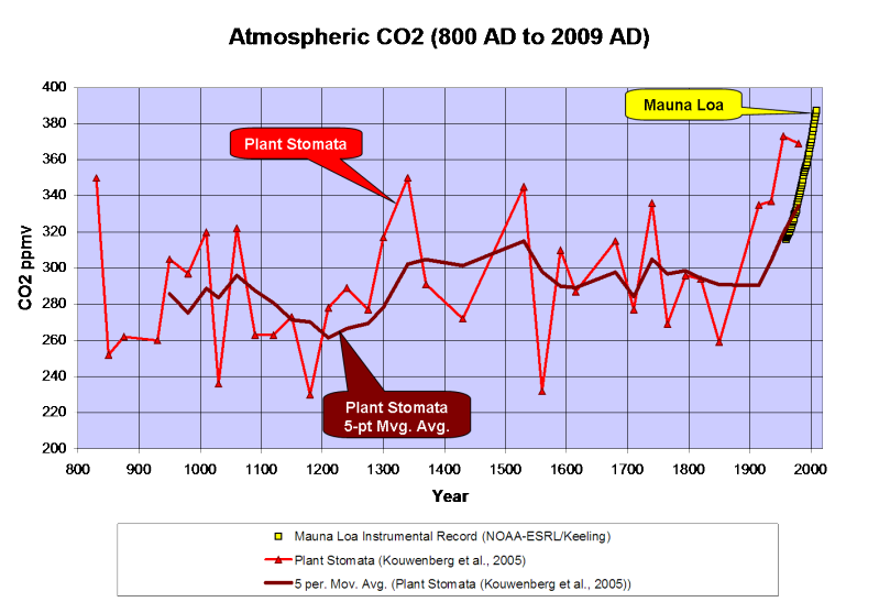
Kouwenberg et al., 2005 found that a “stomatal frequency record based on buried Tsuga heterophylla needles reveals significant centennial-scale atmospheric CO2 fluctuations during the last millennium.”
Plant stomata data show much greater variability of atmospheric CO2 over the last 1,000 years than the ice cores and that CO2 levels have often been between 300 and 340ppmv over the last millennium, including a 120ppmv rise from the late 12th Century through the mid 14th Century. The stomata data also indicate higher CO2 levels than the Mauna Loa instrumental record; but a 5-point moving average ties into the instrumental record quite nicely…

A survey of historical chemical analyses (Beck, 2007) shows even more variability in atmospheric CO2 levels than the plant stomata data since 1800…

WHAT DOES IT ALL MEAN?
The current “paradigm” says that atmospheric CO2 has risen from ~275ppmv to 388ppmv since the mid-1800’s as the result of fossil fuel combustion by humans. Increasing CO2 levels are supposedly warming the planet…

However, if we use Moberg’s (2005) non-Hockey Stick reconstruction, the correlation between CO2 and temperature changes a bit…

Moberg did a far better job in honoring the low frequency components of the climate signal. Reconstructions like these indicate a far more variable climate over the last 2,000 years than the “Hockey Sticks” do. Moberg also shows that the warm up from the Little Ice Age began in 1600, 260 years before CO2 levels started to rise.
As can be seen below, geologically consistent reconstructions like Moberg and Esper are in far better agreement with “direct” paleotemperature measurements, like Alley’s ice core reconstruction for Central Greenland…

In fairness to Dr. Mann, his 2008 reconstruction did restore the Medieval Warm Period and Little Ice Age to their proper places; but he still used Mike’s Nature Trick to slap a hockey stick blade onto the 20th century.
What happens if we use the plant stomata-derived CO2 instead of the ice core data?

We find that the ~250-year lag time is consistent. CO2 levels peaked 250 years after the Medieval Warm Period peaked and the Little Ice Age cooling began and CO2 bottomed out 240 years after the trough of the Little Ice Age. In a fashion similar to the glacial/interglacial lags in the ice cores, the plant stomata data indicate that CO2 has lagged behind temperature changes by about 250 years over the last millennium. The rise in CO2 that began in 1860 is most likely the result of warming oceans degassing.
While we don’t have a continuous stomata record over the Holocene, it does appear that a lag time was also present in the early Holocene…

Once dissolved in the deep-ocean, the residence time for carbon atoms can be more than 500 years. So, a 150- to 200-year lag time between the ~1,500-year climate cycle and oceanic CO2 degassing should come as little surprise.
CONCLUSIONS
-
Ice core data provide a low-frequency estimate of atmospheric CO2 variations of the glacial/interglacial cycles of the Pleistocene. However, the ice cores seriously underestimate the variability of interglacial CO2 levels.
-
GEOCARB shows that ice cores underestimate the long-term average Pleistocene CO2 level by 36ppmv.
-
Modern satellite data show that atmospheric CO2 levels in Antarctica are 20 to 30ppmv less than lower latitudes.
-
Plant stomata data show that ice cores do not resolve past decadal and century scale CO2 variations that were of comparable amplitude and frequency to the rise since 1860.
Thus it is concluded that:
-
CO2 levels from the Early Holocene through pre-industrial times were highly variable and not stable as the Antarctic ice cores suggest.
-
The carbon and climate cycles are coupled in a consistent manner from the Early Holocene to the present day.
-
The carbon cycle lags behind the climate cycle and thus does not drive the climate cycle.
-
The lag time is consistent with the hypothesis of a temperature-driven carbon cycle.
-
The anthropogenic contribution to the carbon cycle since 1860 is minimal and inconsequential.
Note: Unless otherwise indicated, all of the climate reconstructions used in this article are for the Northern Hemisphere.
References
Anklin, M., J. Schwander, B. Stauffer, J. Tschumi, A. Fuchs, J.M. Barnola, and D. Raynaud, CO2 record between 40 and 8 kyr BP from the GRIP ice core, Journal of Geophysical Research, 102 (C12), 26539-26545, 1997.
Wagner et al., 1999. Century-Scale Shifts in Early Holocene Atmospheric CO2 Concentration. Science 18 June 1999: Vol. 284. no. 5422, pp. 1971 – 1973.
Berner et al., 2001. GEOCARB III: A REVISED MODEL OF ATMOSPHERIC CO2 OVER PHANEROZOIC TIME. American Journal of Science, Vol. 301, February, 2001, P. 182–204.
Kouwenberg, 2004. APPLICATION OF CONIFER NEEDLES IN THE RECONSTRUCTION OF HOLOCENE CO2 LEVELS. PhD Thesis. Laboratory of Palaeobotany and Palynology, University of Utrecht.
Wagner et al., 2004. Reproducibility of Holocene atmospheric CO2 records based on stomatal frequency. Quaternary Science Reviews 23 (2004) 1947–1954.
Esper et al., 2005. Climate: past ranges and future changes. Quaternary Science Reviews 24 (2005) 2164–2166.
Kouwenberg et al., 2005. Atmospheric CO2 fluctuations during the last millennium reconstructed by stomatal frequency analysis of Tsuga heterophylla needles. GEOLOGY, January 2005.
Van Hoof et al., 2005. Atmospheric CO2 during the 13th century AD: reconciliation of data from ice core measurements and stomatal frequency analysis. Tellus (2005), 57B, 351–355.
Rundgren et al., 2005. Last interglacial atmospheric CO2 changes from stomatal index data and their relation to climate variations. Global and Planetary Change 49 (2005) 47–62.
Jessen et al., 2005. Abrupt climatic changes and an unstable transition into a late Holocene Thermal Decline: a multiproxy lacustrine record from southern Sweden. J. Quaternary Sci., Vol. 20(4) 349–362 (2005).
Beck, 2007. 180 Years of Atmospheric CO2 Gas Analysis by Chemical Methods. ENERGY & ENVIRONMENT. VOLUME 18 No. 2 2007.
Loulergue et al., 2007. New constraints on the gas age-ice age difference along the EPICA ice cores, 0–50 kyr. Clim. Past, 3, 527–540, 2007.
DATA SOURCES
CO2
Etheridge et al., 1998. Historical CO2 record derived from a spline fit (75 year cutoff) of the Law Dome DSS, DE08, and DE08-2 ice cores.
NOAA-ESRL / Keeling.
Berner, R.A. and Z. Kothavala, 2001. GEOCARB III: A Revised Model of Atmospheric CO2 over Phanerozoic Time, IGBP PAGES/World Data Center for Paleoclimatology Data Contribution Series # 2002-051. NOAA/NGDC Paleoclimatology Program, Boulder CO, USA.
Kouwenberg et al., 2005. Atmospheric CO2 fluctuations during the last millennium reconstructed by stomatal frequency analysis of Tsuga heterophylla needles. GEOLOGY, January 2005.
Lüthi, D., M. Le Floch, B. Bereiter, T. Blunier, J.-M. Barnola, U. Siegenthaler, D. Raynaud, J. Jouzel, H. Fischer, K. Kawamura, and T.F. Stocker. 2008. High-resolution carbon dioxide concentration record 650,000-800,000 years before present. Nature, Vol. 453, pp. 379-382, 15 May 2008. doi:10.1038/nature06949.
Royer, D.L. 2006. CO2-forced climate thresholds during the Phanerozoic. Geochimica et Cosmochimica Acta, Vol. 70, pp. 5665-5675. doi:10.1016/j.gca.2005.11.031.
TEMPERATURE RECONSTRUCTIONS
Moberg, A., et al. 2005. 2,000-Year Northern Hemisphere Temperature Reconstruction. IGBP PAGES/World Data Center for Paleoclimatology Data Contribution Series # 2005-019. NOAA/NGDC Paleoclimatology Program, Boulder CO, USA.
Esper, J., et al., 2003, Northern Hemisphere Extratropical Temperature Reconstruction, IGBP PAGES/World Data Center for Paleoclimatology Data Contribution Series # 2003-036. NOAA/NGDC Paleoclimatology Program, Boulder CO, USA.
Mann, M.E. and P.D. Jones, 2003, 2,000 Year Hemispheric Multi-proxy Temperature Reconstructions, IGBP PAGES/World Data Center for Paleoclimatology Data Contribution Series #2003-051. NOAA/NGDC Paleoclimatology Program, Boulder CO, USA.
Alley, R.B.. 2004. GISP2 Ice Core Temperature and Accumulation Data. IGBP PAGES/World Data Center for Paleoclimatology Data Contribution Series #2004-013. NOAA/NGDC Paleoclimatology Program, Boulder CO, USA.
VEIZER d18O% ISOTOPE DATA. 2004 Update.
“The rise in CO2 that began in 1860 is most likely the result of warming oceans degassing.”
Perhaps a bit premature to accept this conclusion – and it is difficult to believe that all our deforestation and burning of fuel are not contributing. However, if true, then perhaps it really is worse than we thought – the seas must be undergoing alkalinisation (alkalinification?): OMG, we will be swimming in loo cleaner!
p.s. Does this mean corals will disappear as they will not be able to sequester enough carbonate to build their skeletons?
Also, this at least suggests what we can do with all that CO2 which is to be removed from coal-fired emissions – just pump it into the deep oceans to replace what is outgassing at the surface!
This would be much more readable if the bandwidth hadn’t been exceeded at PhotoBucket. No illustrations whatsoever make it hard to understand what is going on…
None of the images are working for me-
“photobucket bandwidth exceeded”
any ideas?
Great post; however, all the images read: “Upgrade to pro today… Bandwidth exceeded… photobucket”. Can’t they simply be uploaded as gif files or whatever? I’d really like to see the graphs instead of images of error messages.
Joel Shore — “If A then B” does not logically-imply “if B then A”.
No kidding. 🙂
Let’s look at a few things:
1. We’re constantly told that the rise from 1800 onward (that’s 200+ years) is anthropogenic. CO2 is up. Temps must therefore rise. It’s so well known that this results in the skeptics reminding all that correlation isn’t causation.
2. Advocates tell us there’s a relationship between temp and CO2. To explain ice core lags (or handwave or whatever) the idea is that if temp goes up CO2 will go up, PERIOD. There is no uptick in temp without an uptick in CO2, and it doesn’t matter which one drive which — there’s a correlation. When one goes up, the other one does.
3. OK, so it’s been pounded in my head by everyone from Gavin S to Andy Lacis to other hangers on that there is a correlation between temp and CO2. No matter what they will follow each other, that they MUST follow, else radiative physics simply doesn’t work.
4. OK, let’s accept this as being true: radiative physics works as explained.
5. The MWP was a warming period. It lasted a couple of centuries. The ice cores show no corresponding CO2 increase (despite the radiative physics people claiming that this MUST happen.)
6. Joel Shore posits a 200 year long volcano or planetary wobble event, claiming “other” forcings.
(Dude. Please.)
7. Conclusion:
a) if temp and Co2 are always intertwined as per radiative physics experts like Lacis, then the ice cores MUST be lying.
b) if the ice cores tell the truth then Lacis is completely wrong.
c) We simply don’t know enough to tell.
Choose.
Bill,
I agree that the stomata data are “noisy” – Most high-frequency data components are noisy. I should have emphasized that point more clearly in my post. The ideal way to use stomata data would be through regional, hemispheric and global averaging… If only there were enough stomata chronologies available.
I should have acknowledged your work in my post. I relied quite a bit on your WUWT post that included a compendium of paleoclimatology data.
Tim,
The ice cores are generally drilled in areas of stable ice… With little lateral movement. Most of the villages that were buried during the onset of the Little Ice Age were buried (more like bulldozed) by advancing glaciers. If you can point me to an article on man-made things buried in ice that seems too old, I’ll try to answer your challenge more thoroughly.
The aging of the ice layers is not particularly difficult, provided the ice has not been deformed.
Leif, well said. That ice cores seem to show a huge lag is not evidence of a cause. The goodies are in the noise and variations. Too much filtering, or using a proxy insensitive to short term variations, leaves us with a dearth of information that could be a gold mine.
Richard,
I agree. Plant stomata data are far from infallible and that many taxa are not useful as CO2 proxies. That’s why botanists like Lenny Kouwenberg, Rike Wagner, Wolfram Kürschner, and Henk Visscher take great care to find taxa that are sensitive to CO2 variations. They build “training sets” from extant and herbarium samples that they calibrate to atmospheric CO2 levels.
Bart says:
In fact, the correlation is very good at low frequencies. Knorr et al. ( http://radioviceonline.com/wp-content/uploads/2009/11/knorr2009_co2_sequestration.pdf ) Figure 1 is a graph showing the relation between the growth rate in CO2 levels in the atmosphere and a curve representing 46% of our annual emissions. Note that since this is plotting the growth rate, i.e., the derivative of CO2 atmospheric concentration vs time, it is a much more sensitive test than if just CO2 atmospheric concentration vs time were compared to commulative emissions. (I have seen such a plot before but can’t find it now.)
As for the correlation at high frequencies, on such short timescales the variations in sequestration rate are larger than the variations in emissions and hence dominate things. Nobody expects it to be otherwise.
The sequestering results in a rapid partition of the CO2 emitted into the atmosphere into the ocean mixed layer and the biosphere. However, after the rapid equilibration occurs amongst these 3 subsystems, only much slower processes operate to sequester the remainder of the CO2 (e.g., in the deep oceans). This is well-understood by all scientists studying the carbon cycle.
In fact, the trend in the growth rate in the Mauna Loa data is clearly upward in time. Perhaps if one looks over short enough times where the variability of uptake is a significant enough factor, one can cherrypick start and end dates that make it seem like such a deceleration is occurring. However, a careful analysis of the data over times long enough to get statistically-significant measures of the growth rate show it is increasing in time: http://web.archive.org/web/20080822110546/tamino.wordpress.com/2008/08/08/yet-more-co2/
If you really believe that such exoneration will occur (i.e., that humans will be found not to be responsible for the large majority of the atmospheric increase in CO2 since the start of the industrial revolution), you could make a lot of money on this notion since there are plenty of people, myself included, that would be more than happy to bet you on this.
Springer,
The amount of anthropogenic CO2 is fairly well accounted for. The natural carbon flux is, at best, a gross estimate.
Mankind puts 6 to 8 GtC worth of CO2 into the atmosphere every year. Plant respiration accounts for 40 to 50 GtC, residuum decay accounts for 50 to 60 GtC and sea-surface gas exchanges accounts for 100 to 115 GtC. The total range of natural sources is 190 to 235 GtC. Anthropogenic emissions are less than 1/5 of the annual variability of the natural sources. Furthermore, ~60% of the annual anthropogenic emissions are taken up by sinks. A~ 60% decay rate (Knorr, 2009) fits right in with the well-established atmospheric residence time of ~15 years. Anthropogenic CO2 emissions simply cannot be staying in the atmosphere long enough to be the primary cause of the CO2 rise since 1860.
The plant stomata and Greenland ice core data both show Preboreal CO2 levels of 350-360 ppmv. The stomata data show CO2 levels routinely rose to 330-360 ppmv in response to prior Holocene warming periods. Every line of evidence, apart from the Antarctic ice cores suggests that atmospheric CO2 levels would be at least 330 ppmv and possibly as high as 360 ppmv without the anthropogenic component. The residence time and decay rate, make it very difficult for the instantaneous anthropogenic component of atmospheric CO2 to be much more than 10 ppmv.
Man is unlocking about 5 to 6 GtC worth of CO2 from fossil storage every year; and this CO2 is being added to the carbon cycle. I have a hunch that the sea-surface gas exchange rate has probably accelerated over the last 150 years… Although I am not aware of any long-term, direct measurements of that exchange rate.
Hi Dave,
very interesting. So how do you counter people such as Ferdi Englebeen who say that the d13-d12 ratio is a slam dunk for proving half the additional airbourne co2 can be attributed to man because of the ‘fingerprint’ of fossil fuel C3 plant material?
Dr. Shore,
I’m not suggesting that anyone “believe” any one data-set over any other. I’m suggesting that we use all of the data and assemble those data in a spectrally consistent manner.
GEOCARB = Woofer,
Ice Cores = Mid-Range
Stomata = Tweeter
On the AIRS data… If you look at the raw, unprocessed, un-smoothed, un-averaged images, the pixels in the Polar regions are generally 365-370 ppmv and the pixels in continental areas in temperate latitudes are greater than 380 ppmv.
I probably should say that the AIRS data show that atmospheric CO2 levels in Antarctica can be 10 to 20 ppmv less than lower latitudes.
IIRC Dr. Henson’s “greenhouse runaway” tripping point is at CO2 = 450ppm.
The GEOCARB data shows this value exceeded by most of the time in the last 600 mya, by a large margin. Two Ice ages occurred with CO2 > 2000 ppm. This is why I’ve been a CO2 doom skeptic for a long time.
******
Leif Svalgaard says:
December 26, 2010 at 6:37 pm
With the CO2 in ice cores so uncertain what is then with the oft repeated statement that CO2 lags temperatures by 800 years? It would seem that that now is not on firm ground.
******
Yeah, that’s a pretty important question. Maybe Ferdinand has some idea — he seems to know some of the estimated inclusion time-lags at the various ice-core sites.
Tim,
Good point on GEOCARB… Pleistocene-aged Antarctic ice cores probably should show lower CO2 levels than a 10-million year moving average over the Neogene. I think that was the point I was trying to make.
Here’s a plot of Neogene CO2 and Temp. GEOCARB indicates that over the last 25 million years, the long-term average of atmospheric CO2 levels declined from ~340 ppmv to ~270 ppmv. Plant stomata “snapshots” show CO2 levels varying from 270 to 370 ppmv over the last 15 million years.
On the Anklin paper, I suggest you actually read the paper, rather than just the abstract. Figure 1 shows CO2 measurements from the GRIP core as high as 340 ppmv and Table 1 shows 331 (+/1 7) ppmv in the Dye 3 core during the Preboreal.
Tallbloke,
That’s on my “to do” list. Somewhere on my thumb-drive, I have a couple of good papers on the d13/d12 ratio doing something every similar in the early Holocene. I just can’t recall where I filed them… My record-keeping is often on par with the CRU… 😉
$24.95 on my Discover Card… Bandwidth restored… 😉
Dr. Svalgaard,
In my opinion, the uncertainty with the ice core aging isn’t so much with the age of the gas bubbles, it’s with the age of the gas in the bubbles.
There is a variable lag time between when the snow is deposited and when the pore throats close off. I think the firen densification model does a pretty good job in estimating the lag time between deposition and “lithification.” So, the ~800-yr average lag time is probably reasonable.
To me the uncertainty is the mix of air that winds up being trapped in those bubbles. In areas of low accumulation rates, it can take 2,000 years or more for enough snow to accumulate and “lithify” the firn. These low accumulation rate areas are also the best candidates for obtaining ice cores with long record lengths. Due to the long period between burial and “lithification,” it seems to me that the trapped air would be a blend of older air that had permeated upwards, contemporaneous air that was buried in the original snow fall and younger air that had permeated downward.
I think that Van Hoof et al., 2005 really pins this down by reconciling the stomata and ice core data through the use of a low frequency filter on the stomata data.
@Middleton
If you won’t let facts get in the way of your beliefs there’s little point in arguing with you. If the oceans were outgassing the surface water would becoming more alkaline. Can you cite any studies that show it?
Stomata density varies in response to light, water, and nutrient levels not just CO2. Studies all show it. Google it. It’s no more reliable as CO2 proxy than tree ring width used as a proxy for temperature.
The bottom line is that increase in atmospheric CO2 is quite consistently about half of annual anthropogenic CO2. That is consistent with an increase in partial CO2 pressure at the ocean/atmosphere interface where the anthropogenic contribution throws it out of equilibrium and the ocean simply isn’t returning to equilibrium as fast as we are moving it away from equilibrium.
One might can try to dispute this but one appears as a crank when they do and it makes the reasonable CAGW skeptics look bad. There are far more questionable aspects of the CAGW hypothesis to dispute than basic things like CO2 increase being anthropogenic in origin and CO2’s ability to raise surface equilibrium temperature via it’s experimentally proven action as an insulator.
G.L. Alston says:
December 27, 2010 at 5:37 am
Temps must therefore rise only if everything else remains constant. It isn’t correlation. It’s fundamental physical law known for 200 years and experimentally demonstrated by John Tyndal 150 years ago. The problem is everything else doesn’t remain constant. Tyndal had to be very careful to dry the gases in the thousands of experiments he ran because water vapor was such a good absorber of thermal radiation he couldn’t otherwise detect the thermal absorption properties of any other gases when water vapor at normal atmospheric concentration was present. On a planet where 70% of the surface presents liquid water and surface pressure is 14psi the water cycle caps how warm the surface can become when incoming radiation at the top of the atmosphere remains nearly constant. Non-condensing greenhouse gases put a bottom on how cold the surface can become when ice becomes the dominant surface presentation. Today we are at a tipping point but that tipping point is towards a surface presentation dominated by ice. CO2 partial pressure is far too low to keep the ice away. It’s insane to want it even lower. The periods of great biological fecundity and many tens of millions of years at a stretch without an ice age are marked by CO2 partial pressures of 2000 ppm or more.
The CAGW boffins are the ones in denial. They are in denial of 500 million years of history contained in the geologic column. They are in denial of the water cycle’s action in capping how warm the surface can become. They are in denial of the biological fecundity that happens when CO2 partial pressure is vastly higher than today.
Joel Shore says:
December 27, 2010 at 7:20 am
“In fact, the correlation is very good at low frequencies. Knorr et al.”
Wow. Least squares curve fits are robust. What a revolutionary discovery!
“As for the correlation at high frequencies, on such short timescales…”
Do a cross correlation. Out of dozens of discernible harmonics, there is only one tiny one with a roughly 20 year period which appears that it could correlate.
“The sequestering results in a rapid partition of the CO2 emitted into the atmosphere into the ocean mixed layer and the biosphere. However, after the rapid equilibration occurs amongst these 3 subsystems, only much slower processes operate to sequester the remainder of the CO2 (e.g., in the deep oceans).”
If that were true, the Earth would never have reached equilibrium, and CO2 concentration from a given instant over a long span of time would effectively be a random walk with variability increasing as the square root of time.
“This is well-understood by all scientists studying the carbon cycle.”
You mean, this narrative is well-understood by these scientists. But, where is the proof?
“In fact, the trend in the growth rate in the Mauna Loa data is clearly upward in time.”
I am not speaking of the trend, but of the acceleration, the trend of the trend. The data are clear and unambiguous.
“However, a careful analysis of the data over times long enough to get statistically-significant measures of the growth rate show it is increasing in time.”
Not even close. Your source is – how to put this delicately? – not reliable.
“Wow. Least squares curve fits are robust. What a revolutionary discovery!”
But, for all that, the fit is still poor.
Dave Middleton:
But, the GEOCARB “data” isn’t really empirical data at all. It is a simulation and my guess is that the author of that model might freely admit that he adjusted things to get the current CO2 levels approximately right and that using any discrepancy between the approximate level and the actual average level is thus circular reasoning. Even if this were not the case, I would imagine he would admit that the errorbars on the estimates from the model are quite large…Certainly the errorbars that he shows going back in time over hundreds of millions of years are very large.
As for the stomata data giving us the high-frequency component: What it seems to give us is a lot of high-frequency NOISE.
That’s a little more reasonable but is likely still too high an estimate for several reasons:
(1) There is presumably a reason why they process the data. Perhaps what you are seeing before the processing is noise?
(2) As has been noted, the ice core data acts as a somewhat-low-pass filter, so it would presumably be doing some averaging and smoothing over time…another reason why looking at the unprocessed data would exaggerate the differences with latitude.
(3) As I noted, the rapid rise in CO2 that is occurring likely means that the spatial variations are larger now than they were during periods when such a rapid rise was not occurring.