Guest post by David Middleton
INTRODUCTION
Anyone who has spent any amount of time reviewing climate science literature has probably seen variations of the following chart…

A record of atmospheric CO2 over the last 1,000 years constructed from Antarctic ice cores and the modern instrumental data from the Mauna Loa Observatory suggest that the pre-industrial atmospheric CO2 concentration was a relatively stable ~275ppmv up until the mid 19th Century. Since then, CO2 levels have been climbing rapidly to levels that are often described as unprecedented in the last several hundred thousand to several million years.
Ice core CO2 data are great. Ice cores can yield continuous CO2 records from as far back as 800,000 years ago right on up to the 1970’s. The ice cores also form one of the pillars of Warmista Junk Science: A stable pre-industrial atmospheric CO2 level of ~275 ppmv. The Antarctic ice core-derived CO2 estimates are inconsistent with just about every other method of measuring pre-industrial CO2 levels.
Three common ways to estimate pre-industrial atmospheric CO2 concentrations (before instrumental records began in 1959) are:
1) Measuring CO2 content in air bubbles trapped in ice cores.
2) Measuring the density of stomata in plants.
3) GEOCARB (Berner et al., 1991, 1999, 2004): A geological model for the evolution of atmospheric CO2 over the Phanerozoic Eon. This model is derived from “geological, geochemical, biological, and climatological data.” The main drivers being tectonic activity, organic matter burial and continental rock weathering.
ICE CORES
The advantage of Antarctic ice cores is that they can provide a continuous record of relative CO2 changes going back in time 800,000 years, with a resolution ranging from annual in the shallow section to multi-decadal in the deeper section. Pleistocene-age ice core records seem to indicate a strong correlation between CO2 and temperature; although the delta-CO2 lags behind the delta-T by an average of 800 years… 
Ice cores from Greenland are rarely used in CO2 reconstructions. The maximum usable Greenland record only dates as far back as ~130,000 years ago (Eemian/Sangamonian); the deeper ice has been deformed. The Greenland ice cores do tend to have a higher resolution than the Antarctic cores because there is a higher snow accumulation rate in Greenland. Funny thing about the Greenland cores: They show much higher CO2 levels (330-350 ppmv) during Holocene warm periods and Pleistocene interstadials. The Dye 3 ice core shows an average CO2 level of 331 ppmv (+/-17) during the Preboreal Oscillation (~11,500 years ago). These higher CO2 levels have been explained away as being the result of in situ chemical reactions (Anklin et al., 1997).
PLANT STOMATA
Stomata are microscopic pores found in leaves and the stem epidermis of plants. They are used for gas exchange. The stomatal density in some C3 plants will vary inversely with the concentration of atmospheric CO2. Stomatal density can be empirically tested and calibrated to CO2 changes over the last 60 years in living plants. The advantage to the stomatal data is that the relationship of the Stomatal Index and atmospheric CO2 can be empirically demonstrated…

When stomata-derived CO2 (red) is compared to ice core-derived CO2 (blue), the stomata generally show much more variability in the atmospheric CO2 level and often show levels much higher than the ice cores…

Plant stomata suggest that the pre-industrial CO2 levels were commonly in the 360 to 390ppmv range.
GEOCARB
GEOCARB provides a continuous long-term record of atmospheric CO2 changes; but it is a very low-frequency record…

The lack of a long-term correlation between CO2 and temperature is very apparent when GEOCARB is compared to Veizer’s d18O-derived Phanerozoic temperature reconstruction. As can be seen in the figure above, plant stomata indicate a much greater range of CO2 variability; but are in general agreement with the lower frequency GEOCARB model.
DISCUSSION
Ice cores and GEOCARB provide continuous long-term records; while plant stomata records are discontinuous and limited to fossil stomata that can be accurately aged and calibrated to extant plant taxa. GEOCARB yields a very low frequency record, ice cores have better resolution and stomata can yield very high frequency data. Modern CO2 levels are unspectacular according to GEOCARB, unprecedented according to the ice cores and not anomalous according to plant stomata. So which method provides the most accurate reconstruction of past atmospheric CO2?
The problems with the ice core data are 1) the air-age vs. ice-age delta and 2) the effects of burial depth on gas concentrations.
The age of the layers of ice can be fairly easily and accurately determined. The age of the air trapped in the ice is not so easily or accurately determined. Currently the most common method for aging the air is through the use of “firn densification models” (FDM). Firn is more dense than snow; but less dense than ice. As the layers of snow and ice are buried, they are compressed into firn and then ice. The depth at which the pore space in the firn closes off and traps gas can vary greatly… So the delta between the age of the ice and the ago of the air can vary from as little as 30 years to more than 2,000 years.
The EPICA C core has a delta of over 2,000 years. The pores don’t close off until a depth of 99 m, where the ice is 2,424 years old. According to the firn densification model, last year’s air is trapped at that depth in ice that was deposited over 2,000 years ago.
I have a lot of doubts about the accuracy of the FDM method. I somehow doubt that the air at a depth of 99 meters is last year’s air. Gas doesn’t tend to migrate downward through sediment… Being less dense than rock and water, it migrates upward. That’s why oil and gas are almost always a lot older than the rock formations in which they are trapped. I do realize that the contemporaneous atmosphere will permeate down into the ice… But it seems to me that at depth, there would be a mixture of air permeating downward, in situ air, and older air that had migrated upward before the ice fully “lithified”.
A recent study (Van Hoof et al., 2005) demonstrated that the ice core CO2 data essentially represent a low-frequency, century to multi-century moving average of past atmospheric CO2 levels.

It appears that the ice core data represent a long-term, low-frequency moving average of the atmospheric CO2 concentration; while the stomata yield a high frequency component.
The stomata data routinely show that atmospheric CO2 levels were higher than the ice cores do. Plant stomata data from the previous interglacial (Eemian/Sangamonian) were higher than the ice cores indicate…

The GEOCARB data also suggest that ice core CO2 data are too low…

The average CO2 level of the Pleistocene ice cores is 36ppmv less than GEOCARB…

Recent satellite data (NASA AIRS) show that atmospheric CO2 levels in the polar regions are significantly less than in lower latitudes…


So… The ice core data should be yielding lower CO2 levels than the Mauna Loa Observatory and the plant stomata.
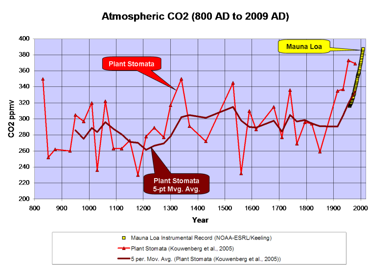
Kouwenberg et al., 2005 found that a “stomatal frequency record based on buried Tsuga heterophylla needles reveals significant centennial-scale atmospheric CO2 fluctuations during the last millennium.”
Plant stomata data show much greater variability of atmospheric CO2 over the last 1,000 years than the ice cores and that CO2 levels have often been between 300 and 340ppmv over the last millennium, including a 120ppmv rise from the late 12th Century through the mid 14th Century. The stomata data also indicate higher CO2 levels than the Mauna Loa instrumental record; but a 5-point moving average ties into the instrumental record quite nicely…

A survey of historical chemical analyses (Beck, 2007) shows even more variability in atmospheric CO2 levels than the plant stomata data since 1800…

WHAT DOES IT ALL MEAN?
The current “paradigm” says that atmospheric CO2 has risen from ~275ppmv to 388ppmv since the mid-1800’s as the result of fossil fuel combustion by humans. Increasing CO2 levels are supposedly warming the planet…

However, if we use Moberg’s (2005) non-Hockey Stick reconstruction, the correlation between CO2 and temperature changes a bit…

Moberg did a far better job in honoring the low frequency components of the climate signal. Reconstructions like these indicate a far more variable climate over the last 2,000 years than the “Hockey Sticks” do. Moberg also shows that the warm up from the Little Ice Age began in 1600, 260 years before CO2 levels started to rise.
As can be seen below, geologically consistent reconstructions like Moberg and Esper are in far better agreement with “direct” paleotemperature measurements, like Alley’s ice core reconstruction for Central Greenland…

In fairness to Dr. Mann, his 2008 reconstruction did restore the Medieval Warm Period and Little Ice Age to their proper places; but he still used Mike’s Nature Trick to slap a hockey stick blade onto the 20th century.
What happens if we use the plant stomata-derived CO2 instead of the ice core data?

We find that the ~250-year lag time is consistent. CO2 levels peaked 250 years after the Medieval Warm Period peaked and the Little Ice Age cooling began and CO2 bottomed out 240 years after the trough of the Little Ice Age. In a fashion similar to the glacial/interglacial lags in the ice cores, the plant stomata data indicate that CO2 has lagged behind temperature changes by about 250 years over the last millennium. The rise in CO2 that began in 1860 is most likely the result of warming oceans degassing.
While we don’t have a continuous stomata record over the Holocene, it does appear that a lag time was also present in the early Holocene…

Once dissolved in the deep-ocean, the residence time for carbon atoms can be more than 500 years. So, a 150- to 200-year lag time between the ~1,500-year climate cycle and oceanic CO2 degassing should come as little surprise.
CONCLUSIONS
-
Ice core data provide a low-frequency estimate of atmospheric CO2 variations of the glacial/interglacial cycles of the Pleistocene. However, the ice cores seriously underestimate the variability of interglacial CO2 levels.
-
GEOCARB shows that ice cores underestimate the long-term average Pleistocene CO2 level by 36ppmv.
-
Modern satellite data show that atmospheric CO2 levels in Antarctica are 20 to 30ppmv less than lower latitudes.
-
Plant stomata data show that ice cores do not resolve past decadal and century scale CO2 variations that were of comparable amplitude and frequency to the rise since 1860.
Thus it is concluded that:
-
CO2 levels from the Early Holocene through pre-industrial times were highly variable and not stable as the Antarctic ice cores suggest.
-
The carbon and climate cycles are coupled in a consistent manner from the Early Holocene to the present day.
-
The carbon cycle lags behind the climate cycle and thus does not drive the climate cycle.
-
The lag time is consistent with the hypothesis of a temperature-driven carbon cycle.
-
The anthropogenic contribution to the carbon cycle since 1860 is minimal and inconsequential.
Note: Unless otherwise indicated, all of the climate reconstructions used in this article are for the Northern Hemisphere.
References
Anklin, M., J. Schwander, B. Stauffer, J. Tschumi, A. Fuchs, J.M. Barnola, and D. Raynaud, CO2 record between 40 and 8 kyr BP from the GRIP ice core, Journal of Geophysical Research, 102 (C12), 26539-26545, 1997.
Wagner et al., 1999. Century-Scale Shifts in Early Holocene Atmospheric CO2 Concentration. Science 18 June 1999: Vol. 284. no. 5422, pp. 1971 – 1973.
Berner et al., 2001. GEOCARB III: A REVISED MODEL OF ATMOSPHERIC CO2 OVER PHANEROZOIC TIME. American Journal of Science, Vol. 301, February, 2001, P. 182–204.
Kouwenberg, 2004. APPLICATION OF CONIFER NEEDLES IN THE RECONSTRUCTION OF HOLOCENE CO2 LEVELS. PhD Thesis. Laboratory of Palaeobotany and Palynology, University of Utrecht.
Wagner et al., 2004. Reproducibility of Holocene atmospheric CO2 records based on stomatal frequency. Quaternary Science Reviews 23 (2004) 1947–1954.
Esper et al., 2005. Climate: past ranges and future changes. Quaternary Science Reviews 24 (2005) 2164–2166.
Kouwenberg et al., 2005. Atmospheric CO2 fluctuations during the last millennium reconstructed by stomatal frequency analysis of Tsuga heterophylla needles. GEOLOGY, January 2005.
Van Hoof et al., 2005. Atmospheric CO2 during the 13th century AD: reconciliation of data from ice core measurements and stomatal frequency analysis. Tellus (2005), 57B, 351–355.
Rundgren et al., 2005. Last interglacial atmospheric CO2 changes from stomatal index data and their relation to climate variations. Global and Planetary Change 49 (2005) 47–62.
Jessen et al., 2005. Abrupt climatic changes and an unstable transition into a late Holocene Thermal Decline: a multiproxy lacustrine record from southern Sweden. J. Quaternary Sci., Vol. 20(4) 349–362 (2005).
Beck, 2007. 180 Years of Atmospheric CO2 Gas Analysis by Chemical Methods. ENERGY & ENVIRONMENT. VOLUME 18 No. 2 2007.
Loulergue et al., 2007. New constraints on the gas age-ice age difference along the EPICA ice cores, 0–50 kyr. Clim. Past, 3, 527–540, 2007.
DATA SOURCES
CO2
Etheridge et al., 1998. Historical CO2 record derived from a spline fit (75 year cutoff) of the Law Dome DSS, DE08, and DE08-2 ice cores.
NOAA-ESRL / Keeling.
Berner, R.A. and Z. Kothavala, 2001. GEOCARB III: A Revised Model of Atmospheric CO2 over Phanerozoic Time, IGBP PAGES/World Data Center for Paleoclimatology Data Contribution Series # 2002-051. NOAA/NGDC Paleoclimatology Program, Boulder CO, USA.
Kouwenberg et al., 2005. Atmospheric CO2 fluctuations during the last millennium reconstructed by stomatal frequency analysis of Tsuga heterophylla needles. GEOLOGY, January 2005.
Lüthi, D., M. Le Floch, B. Bereiter, T. Blunier, J.-M. Barnola, U. Siegenthaler, D. Raynaud, J. Jouzel, H. Fischer, K. Kawamura, and T.F. Stocker. 2008. High-resolution carbon dioxide concentration record 650,000-800,000 years before present. Nature, Vol. 453, pp. 379-382, 15 May 2008. doi:10.1038/nature06949.
Royer, D.L. 2006. CO2-forced climate thresholds during the Phanerozoic. Geochimica et Cosmochimica Acta, Vol. 70, pp. 5665-5675. doi:10.1016/j.gca.2005.11.031.
TEMPERATURE RECONSTRUCTIONS
Moberg, A., et al. 2005. 2,000-Year Northern Hemisphere Temperature Reconstruction. IGBP PAGES/World Data Center for Paleoclimatology Data Contribution Series # 2005-019. NOAA/NGDC Paleoclimatology Program, Boulder CO, USA.
Esper, J., et al., 2003, Northern Hemisphere Extratropical Temperature Reconstruction, IGBP PAGES/World Data Center for Paleoclimatology Data Contribution Series # 2003-036. NOAA/NGDC Paleoclimatology Program, Boulder CO, USA.
Mann, M.E. and P.D. Jones, 2003, 2,000 Year Hemispheric Multi-proxy Temperature Reconstructions, IGBP PAGES/World Data Center for Paleoclimatology Data Contribution Series #2003-051. NOAA/NGDC Paleoclimatology Program, Boulder CO, USA.
Alley, R.B.. 2004. GISP2 Ice Core Temperature and Accumulation Data. IGBP PAGES/World Data Center for Paleoclimatology Data Contribution Series #2004-013. NOAA/NGDC Paleoclimatology Program, Boulder CO, USA.
VEIZER d18O% ISOTOPE DATA. 2004 Update.
Discover more from Watts Up With That?
Subscribe to get the latest posts sent to your email.
“The rise in CO2 that began in 1860 is most likely the result of warming oceans degassing.”
=============================================
Just like it has always been………………..
David,
thank you for the very interesting post. Could you please modify the images to have links to individual pages? I find that the graphs extend out into the right sidebar and are partially covered by the items in the sidebar. For example, I cannot read the caption on the Wagner et. al. image because it is partially covered by the right sidebar.
Links that open the images in their own pages would solve this minor problem and would be greatly appreciated.
Best regards,
Tom Moriarty
ClimateSanity.wordpress.com
Very nice post. Well thought out. Follows standard research article format. Leaves out emotional baggage on either side. Develops summaries based on the data alone. Written at a level and without jargon, that most can readily understand. Would have been nice to see what further information/data analysis would be useful to investigate.
Might we be able to reconstruct the greening of the planet during these episodes of stomata changes? I am guessing there is a correlate lag similar to CO2 reconstruction. Fossil remnants would be useful to measure this, especially around the supposed edges of such “greening”.
Welcome survey of all to often neglected evidence. A good companion to this post would be Jeffrey Glassman’s paper showing the consistency of the vostok record with Henry’s Law:
http://rocketscientistsjournal.com/2006/10/co2_acquittal.html#more
Interesting and informative and obviously took some time and effort to put together.
Thankyou.
A fascinating post, indeed. I have been searching the net, and have not found an answer to this question–are there instruments currently measuring CO2 anywhere other than Mauna Loa? although it is apparently widely assumed that atmospheric concentrations are homogeneous worldwide, it would be useful to know if there is a second site to provide a backup to Mauna Loa.
[Yes; from c. 100 other sites wordwide. The CO2 data itself does not seem to be the problem. Rather, the effect of CO2 seems to be the issue. ~ Evan]
Nice breakdown. I’ve been questioning the ice core data for a while. You do have to marvel at how the major core reference used by the Alarmist side is usually Lonnie Thompson’s, but no one can find his actual data to confirm his work. Makes getting Phil Jones’ homework look simple.
If a layman may ask a stupid question:
Why does the Mauna Loa CO2 readings go up in such a perfectly straight line, in spite of year over year variations in fossil fuel usage, widespread deforestation, and whatever other factors contribute to the amount of CO2 in the Atmosphere.
It just seems that the CO2 levels year over year wouldn’t be such a nice straight line for so many years.
Good post David.
Just one comment: The stomata-based CO2 estimates seem to be generally accurate, but they do exhibit a lot of varibility which means there is a large error margin in the methodology for individual estimates. They should probably be averaged over some longer time period.
Pamela Gray says:
December 26, 2010 at 9:04 am
Might we be able to reconstruct the greening of the planet during these episodes of stomata changes? I am guessing there is a correlate lag similar to CO2 reconstruction. Fossil remnants would be useful to measure this, especially around the supposed edges of such “greening”.
I too have wondered aloud as to this question. I would imagine that someone has at some point thought of coming at the CO2 conundrum from the other direction; if not to show causation then then for little more than curiosity?
Great analysis, many thanks for this.
The article was most interesting. However, I find the two directions of time on the x-axes presented in the graphs to be confusing or difficult to compare. In some cases, time to the present goes to the left, and in the other cases, time to the present goes to the right. Most of the contemporary charts such as the little ice ages or the hockey stick have the present ending on the right. But the ice core graphs have the present starting on the left.
Excellent post, David. I’ve read about the 3 methods individually but this is the first time I’ve seen all three discussed together. Very easy to read and understand. Thank you.
“The age of the layers of ice can be fairly easily and accurately determined”
I challenge this. They still cannot explain how things that they think should be hundreds if not thousands of years old in Greenland can be buried as deep as they are from past settlements and even airplanes! If there is an explanation of this then give me the link.
Wow! So thorough, so methodical, very impressive. You should publish it in a peer reviewed publication.
Stomata-based estimates of CO2 concentration are far from infallible. Indeed, for some species, there is little or no correlation between stomatal density and CO2 concentration.
See Eide & Birks 2004 Stomatal frequency of Betula pubescens and Pinus sylvestris shows no proportional relationship with atmospheric CO2 concentration http://onlinelibrary.wiley.com/doi/10.1111/j.1756-1051.2004.tb00848.x/abstract
Pamela Gray says:
December 26, 2010 at 8:58 am
Written at a level and without jargon, that most can readily understand.
Yes, very well done.
Thanks David.
David:
Great review of the three methods of paleo CO2 determinations.
Looks like C3 stomata provides a good method for high resolution CO2 measurements. Pity that the spatial and temporal resolution is so spotty. Clearly more work needs to be done, and I hope that those doing the research are not being hobbled by the funding bosses due to the inconvenient results.
Excellent post David. Have there been any studies done on refining models for the upward and downward diffusion of gasses in ice pores, using nuclear tagging provided by above-ground nuclear testing during the 1950s?
Just precisely why do you exaggerate the behavior of CO2 in the first figure by leaving out the bottom of the scale? The true shape of the curve can only be seen if you start the vertical scale from zero instead of from 230. These tricks should not be employed if you want to be objective in your presentation.
From one geoscientist to another: nice piece of work.
Thanks for putting this together.
Great article!
Very educational and well structured. I cant find out whether the CO2 measurements from Mauna Loa takes into account that the CO2 levels are lower at the poles than over lower latitudes. Otherwise they are comparing apples and oranges in thier statistics.
@ur momisugly tommoriarty: If you will right click on the image, you may select view image or open image. That works in Firefox, Opera and Chrome/Safari. I have no clue how to do it in IE.
cheers,
gary
David,
Thank you for your excellent, well presented post.
I have rarely learnt so much in an hour or so than by reading it, although I have to admit my ignorance of a few items.
If I may make so bold, I have arrived at the following…
Temperature in the oceans varies in different areas, hence dissolved CO2 in sea water varies in different oceans;
atmospheric concentrations of CO2 vary geographically;
different methods of measuring past CO2 levels (ice cores & plant stomata) can result in huge variations – >50% at times, although GEOCARB may provide a ‘steadier’ historical record;
there are difficulties in measuring the age of air:ice, and the effects of gas compression at depth;
temperature variation precedes CO2 level variation, upwards or downwards.
Aside from the last point, if I am correct in assuming the others are true, then it would appear that yet more complication is prevalent.
Speaking for myself, the more one delves deeper into any particular aspect of climate, the more one realises how little is known of the whole.