Guest post by Steve Goddard
UPDATE 1-15-08:
I tried an experiment which some of the null questioners may find convincing. I took all of the monthly data from 1978 to 1997, removed the volcanic affected periods, and calculated the mean. Interestingly, the mean anomaly was positive (0.03) i.e. above the mean anomaly for the 30 year period.
This provides more evidence that normalizing to null is conservative. Had I normalized to 0.03, the slope would have been reduced further.
Yesterday’s discussion raised a few questions, which I will address today.
We are all personally familiar with the idea that reduced atmospheric transparency reduces surface temperatures. On a hot summer day, a cloud passing overhead can make a marked and immediate difference in the temperature at the ground. A cloudy day can be tens of degrees cooler than a sunny day, because there is less SW radiation reaching the surface, due to lower atmospheric transparency.
Similarly, an event which puts lots of dust in the upper atmosphere can also reduce the amount of SW radiation making it to the surface. It is believed that a large meteor which struck the earth at the end of the Cretaceous, put huge amounts of dust and smoke in the upper atmosphere that kept the earth very cold for several years, leading to the extinction of the dinosaurs. Carl Sagan made popular the idea of “nuclear winter” where the fires and dust from nuclear war would cause winter temperatures to persist for several years.
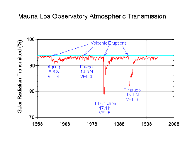
Large volcanic eruptions can have a similar effects. This was observed in 1981 and 1992, when volcanic eruptions caused large drops in the measured atmospheric transmission of shortwave radiation at the Mauna Loa observatory. These eruptions lowered atmospheric transmission for several years, undoubtedly causing a significant cooling effect at the surface. At one point in late 1991, atmospheric transmission was reduced by 15%. An extended period like that would lead to catastrophically cold conditions on earth.
In recent years, there has been a lot of interest in measuring how much warming of the earth has occurred due to increased CO2 concentrations from burning fossil fuels. This is difficult to measure, but one thing we can do to improve the measurements is to filter out events which are known to be unrelated to man’s activities. Volcanoes are clearly in that category. In yesterday’s analysis, I chose to null out the years where atmospheric transparency was affected by volcanic eruptions, as seen in the image below. Atmospheric transmission is in green, and UAH satellite temperatures are in blue.
Atmospheric transmission in green. Monthly temperature deviation in blue, with overlap periods nulled out.
The question was raised, why did I null out those periods?
I made that decision because the null level is the mean deviation for the period, and because that is the most conservative approach. As you can see in the image below, there is a large standard deviation and variance from month to month, which makes other approaches extremely problematic. There were also corresponding El Ninos during both of the null periods, which would have been expected to raise the temperature significantly in the absence of the the volcanic dust. Had I attempted to adjust for the El Nino events, the reduction in slope (degrees per century) would have been greater than what I reported. This is because the temperature anomaly during each El Nino would have been greater than zero (above the null line.)
Due to the large standard deviation and large monthly variance, any attempt to calculate what the temperature “should have been” in the absence of the volcanic dust would likely introduce unsupportable error into the calculation. One can play all sorts of games based on their belief system about what the temperature should have been. I chose not to do that, and instead used the mean as the most conservative approach.
There is no question that the volcanic dust lowered temperatures during those periods, and because of that the 1.3C/century number is too high. My approach came up with 1.0. A reasonable ENSO based approach would have come up with a number much less than that. If you take nothing else away from this discussion, that is the important point.
UAH, with non-nulled temperatures in green.
Furthermore, it is also important to realize that the standard approach of reporting temperature trends as linear slopes is flawed. Climate is not linear, which is why Dr. Roy Spencer fits his UAH curves with a fourth or fifth order function, rather than a line.
Geoff Sharp,
Shortening up the null period has no effect on the results within the reported precision. Also remember that even a 1% decrease in SW radiation produces more than a 1C difference in average temperature. The peak reduction was 15%.
Speaking of Sagan. I remember him on national TV at the time of the Iraq war stating that Richard Turco had some models that indicated the smoke from the oil well fires would loft to the stratosphere and create catastrophic global cooling. Did anything close to that show up in any of the data? Here is an interesting article that sounds a lot like current rhetoric I see about global warming.
http://www.anomalies.net/archive/Fringe-Political_Belief/KUWAITEV.TXT
Steve,
Nulling the data during the volcanic periods is not ideal, but it is not terrible either. Having said that, you did not *null* the data points. You set them equal to zero. Why did you not just remove them from the calculation? That would make a lot more sense.
As for the El Ninos during the volcanic periods, correcting for El Nino would decrease the temperatures (just as correcting for volcanoes would increase the temperatures). Decreasing the temperatures near the start of the period would *increase* the trend. You report that “the reduction in slope (degrees per century) would have been greater than what I reported” if you “attempted to adjust for the El Nino events”. That’s just plain wrong.
“..It is a bit early in the year to staking out a position in the race for boneheaded move of the year in the climate wars, but NASA GISS has done just that but doubling down on its prediction that 2009 or 2010 will be the warmest on record…”
If I were in charge of producing a set of figures and you asked me to bet on whether the figures would go up or down, I would happily take your money. But then, I am a bit dodgy….
Richard111 (05:44:48) :
“OK, I am still confused. Why did my kids get sunburnt on completely overcast day?”
The burning UV rays can still penetrate the clouds. The problem is that because you do not feel as much intensity from the other energy you are not as uncomfortable and can tolerate the heat better. This false comfort zone tends to make people remain outside and consequently stay exposed too long.
I tried an experiment which some of the null questioners may find convincing. I took all of the monthly data from 1978 to 1997, removed the volcanic affected periods, and calculated the mean. Interestingly, the mean anomaly was positive (0.03) i.e. above the median for the period.
This provides more evidence that normalizing to null is conservative. Had I normalized to 0.03, the slope would have been reduced further.
Katherine says:
However, the problem with this argument is that it is very dependent on the period we look at. Yes, it is true that the effect of removing a few cold years in the first half of the 1979-2008 satellite record is to lower the trend over that period. However, if you looked over the period of, say, 1970 to 1994, then removing this data would be removing data in the second half of the period and it would make that slope greater. (Unfortunately, we don’t have satellite data before 1979 although we do have surface data.)
And, if you looked at a longer period of, say, 1970 to 2008, removing that data would probably make essentially no change in the trend.
Worse yet, Steve’s whole analysis has assumed that we can remove the effect of volcanoes simply by removing a short period of a year or two after the eruption. However, volcanoes presumably do have a small longer term effect on the climate too…and this effect would be to make things cooler than they would otherwise be. So, in fact, in the absence of these major volcanic eruptions, we would expect the temperature trend to have been somewhat higher than it is.
So, in other words, by restricting the time period over which he considers the trend…and by assuming the effect of volcanoes is only over a short period with absolutely no effect over the longer term, Steve has managed to convert a natural process that would generally tend to lower the temperature trend over what it would be in the absence of that process to one that does the reverse.
“Given our expectation of the next El Niño beginning in 2009 or 2010, it still seems likely that a new global temperature record will be set within the next 1-2 years, despite the moderate negative effect of the reduced solar irradiance.”
This expectation is rather obviously a WAG, not even one involving looking at past history, a la D’Aleo, where with negative PDO, 60% of the next 30 years will endure La Nina conditions. The remaining 40% will be split between neutral and El Nino conditions.
Whistlin’ past the graveyard…Jimbo forecast a super El Nino for 2007. How’d that work out? “Dead? He’s worse than dead, Jim!”
David Douglas emailed me back with a link to the paper that was missing in the first comment of part1
Anthony;
The link to the paper “Limits on CO2 Climate Forcing from Recent Temperature Data of Earth” is
http://arxiv.org/abs/0809.0581
Also a copy is attached.
Regards;
David Douglass
Sorry, the second paragraph in the blockquote of my previous post should be attributed to “Tom in chilled Florida”. Only the first paragraph is from Katherine.
Steve Goddard says:
While it may be true that we don’t expect exactly a linear relation, over a short enough time the higher order terms are unlikely to be that significant (i.e., all functions are locally linear over some period as long as you are not right at a point of zero slope). Fitting a higher order function just results in overfitting of the data. At the moment, you folks like this overfitting since, due to the La Nina, it tends to produce significant downward curvature near the endpoint. However, once we have the next El Nino and such a high order polynomial fit yields upward curvature near the endpoint, it will be interesting to see if you in the “skeptic” community are still singing the praises of these higher order fits!
Anthony — I didn’t realize you were holding comments for moderation.
Is that normal for everyone or am I being held for some reason?
Thanks.
Reply: It’s not personal. Anthony is sick, I went shopping, and the other moderators probably had something come up. Occasionally that happens. All posts are current now. ~ dbstealey, mod.
Pearland Aggie:
If you cool the past, then you warm the present. (Obviously, you already know this.) I fully expect to see higher highs in the GISS data for 2009 or 2010 in the event of a run-of-the-mill El Nino. My prediction is that the adjusters will adjust their adjustments just enough to do the trick.
One thing that everybody keeps missing is that the GISS data set shows higher highs whereas the others do not. From a public relations (psy-ops) perspective, this is a highly significant difference. One could argue that it is the only thing that matters. The public doesn’t care if the difference is statistically insignificant or within one standard deviation. A higher high means big bold headlines splashed on newsprint and computer monitors all over the world. It sets the narrative, which in turn affects funding, livelihoods, regulations and who knows what else. It’s the narrative that counts. The earth could be entering a new mini-ice age for all we know but it doesn’t matter if people don’t believe it.
Willem, good buddy. Let me try to explain what the paper is saying:
The objective is to find the correct temperature TREND–the SLOPE. Not what the global temperature IS, but whether it is going up or down or level, and by how much–what is the angle?
The angle (the ‘slope’) is set by the total area of the T line on each side of the midpoint year, which is similar to the center-of-gravity of the data:
There are five kids on each end of a teeter-totter, four fat (hot), one thin (cold). If you take the thin kid off the left end of the teeter-totter, the right end goes down. The slope is lower.
Trying to account for the missing heat isn’t relevant to the slope. Factoring in the missing heat is like lowering the entire teeter-totter a half inch closer to the ground. That doesn’t effect the SLOPE.
Janama: FYI, there are about 200,000 sub-sea volcanoes.
«You can’t “remove years” from the analysis. That would make the slope artificially steep, and the data set meaningless. »
You lost me there. Removing data points during periods where you know your measures are affected is what is done in most fields of science.
You can check that with a situation where there are no errors to mess up things:
x=[1,2,3,4,5]
y=[1,2,3,4,5]
If you fit them to
y=a*x+b
One gets, a=1, b=0
Removing the points with x=[2,3] from the data set won’t change the slope from the fit.
x=[1,4,5]
y=[1,4,5]
still has a slope of 1.
But replacing those same points with y=3, that is using the y average for two of them:
x=[1,2,3,4,5]
y=[1,3,3,4,5]
gets you a slope of 0.9
Using the mean is still a biased approach: you are replacing a trended set of points with a non-trended one. One should simply not use those years when computing the slope.
I forget to tell I was using regular least-squares, with no weighting.
The Douglass and Christy paper contains a series of invalid assumptions. The most obvious being that the calculations are based on just the tropics, having rejected the Global, Northern and Southern extratropic anomalies because the Northern extratropics show more rapid warming than the tropics or the globe.
“However, it is noted that NoExtropics is 2 times that of the global and 4 times that of the Tropics. Thus one concludes that the climate forcing in the NoExtropics includes more than CO2 forcing. …”
Does one also conclude that everywhere else its pure CO2 and nothing else?
The global values, however, are not suitable to analyze for that signal because they contains effects from the NoExtropic latitude band which were not consistent with the assumption of how Earth’s temperature will respond to CO2 forcing.
1. The effect of the oceans and heat uptake is ignored, the thermal inertia and differential heat capacity of land and sea explain most of the different rates of warming in different latitudes. There is a higher proportion of ocean in the tropics and hence a slower temperature response. Pretty basic stuff. Globally, the effect of oceans is to add a delay to temperature response to forcing.
2 Polar amplification: The paper fails to acknowledge the predicted and observed property of the global climate system that produces greater relative warming at high latitudes due to snow + ice albedo feedback as well as the higher relative land surface area.
In other words – the glaring error is to assume that a globally uniform forcing from well-mixed CO2 should produce a uniform temperature change The more rapid warming in the North is an expected consequence of the greater proportion of land, with its lower heat capacity, than the mainly oceanic South, rather than evidence that other forcings are at work.
You would expect a paper that demonstrates that a key conclusion of the IPCC is wrong would have generated something of a scientific storm … I’d be interested to learn if this was submitted/accepted anywhere other than Energy & Environment?
Joel Shore (08:05:45) :
While it may be true that we don’t expect exactly a linear relation, over a short enough time the higher order terms are unlikely to be that significant (i.e., all functions are locally linear over some period as long as you are not right at a point of zero slope). Fitting a higher order function just results in overfitting of the data. At the moment, you folks like this overfitting since, due to the La Nina, it tends to produce significant downward curvature near the endpoint. However, once we have the next El Nino and such a high order polynomial fit yields upward curvature near the endpoint, it will be interesting to see if you in the “skeptic” community are still singing the praises of these higher order fits!
Fair enough.
By way of rebuttal, here are a few observations and my concern:
1. The average value of a sine wave is zero.
2. Very nearly 50% of the time amplitude is increasing.
3. Very nearly 50% of the time amplitude is decreasing.
My concern is that some persons lacking in ethics might take a period when the sine wave is increasing in amplitude, “extrapolate” a linear progression, and claim that the amplitude would continue increasing for a long time to very large values. Furthermore, they might claim this was reasonable, since over some period it’s locally linear. Even worse, in the real world, some individuals with ulterior motives might manipulate the measurements of the amplitude in order to hide the fact that the real world phenomena was oscillating.
BTW, I think you’ll find our response to an upward curvature to be along the lines of “now the climate’s in a warming period.” The denial you’re projecting is on the other side of this issue.
Steven Goddard,
Firstly, it is self-evident that if you remove below average data from the first half of a rising linear trend then you will reduce its pitch. However, the opposite is equally true: thus if you were to null out these same periods from a linear trend of temperatures from the beginning of the 20th century you would increase the linear warming trend.
Secondly, as has been pointed out already, you would need to be able to show that you have only removed below average data which is solely attributable to volcanic aerosol cooling . You are a long way from doing that, and the presumption that ‘zero’ is a fair value to enter for a substitution of data in the first half of a rising trend is obviously unsound (you seem to confuse the mean for a period with the expected value for data points within that period).
Thirdly, you state that you have set the flat-lined periods to the mean. However, this mean was calculated including the data from those periods and would be a different figure if that data had actually been flat-lined according to your substitution. So, even apart from the fact of my second point, your recalculation of trend is without useful accuracy.
I think it is reasonable to say that if one could calculate how to remove natural negative forcings from the first half of the period in question it would reduce that period’s warming trend (whilst increasing the trend of the longer record). However, it would also be reasonable to say that removal of negatives from the latter part of the period would increase the warming trend – the reduction in solar output and the 2008 La Nina, for example. Why is it that you have only mentioned considering the removal of a warming influence from the latter part – the 1998 El Nino, that is? It would appear that you have only considered adjustments that would reduce the warming trend for the period you are considering. Is that confirmation bias on your part, or, if not, how do you account for it?
Filipe (08:48:55) : “…Removing data points during periods where you know your measures are affected is what is done in most fields of science. You can check that with a situation where there are no errors to mess up things:
x=[1,2,3,4,5]
y=[1,2,3,4,5]”
Your statement is incorrect, Filipe, and your example, is way off the mark. A high school algebra exercise won’t cover the situation. The thesis here involves a timeline. You can’t just scissor out extraneous data and close up the gap; to do that, you have to scissor out part of the abscissa, as well. Using your analogy, you’d be left with:
x=[3,4,5] (2 and 3 no longer exist, The abscissa value formerly known as 1 has been moved up adjacent to 4)
y=[1,4,5],
which does have a different slope.
Besides, climate science doesn’t just “remove data points,” Fililpe. From what I’ve seen, there’s a tendency to make new ones up, instead.
The relationship between warm / cool periods of Earth’s history is, I suppose, at the hear of the ongoing discussion here. I believe one of the sleaziest tricks of the climatologists, and a cause of a lot of our (mis)conceptions about climate is the “(mis)framing” of the period of time we’re referring to. Not to be seen on Wikipedia is the following perspective on Paleoclimate, at the 500 million year level. (Please scroll down to the graph in “Ice House or Hot House?”)
http://www.scotese.com/climate.htm
Scotese is (also) an artist whose work appear(s) (or used to) on paleo exhibits at the Denver Museum of Nature and Science. His method of researching the graph was to study the movement of the continents and the types of rocks formed at different phases of the planet’s development. Read more here http://www.scotese.com/climate1.htm for his “Methods Used to Determine Ancient Climates”.
Finally, an astute blogger at “Free Republic” superimposed an equally long record of atmospheric CO2 onto Mr. Scotese’ temp graph to provide an interesting insight: there appears to be little correspondence. (I don’t know how the Paleo – CO2 record was determined). See link below.
I agree with you that Earth’s temperature over geological time scales is constantly fluctuating. But following the logic of this research, Earth is likely to experience warmer times in the next few million years whether people are around to see it or not.
http://www.freerepublic.com/focus/f-news/1644060/posts
Well we might get the opportunity to investigate volcanic cooling in real time, USGS is reporting a quake in eastern Russia , Magnitude 7.3 – EAST OF THE KURIL ISLANDS.
If the so called champagne effect is real this might be intense enough to cause some activity in the Aleutian island volcanoes.
No word yet on any significant details location = 46.888°N, 155.167°E
http://earthquake.usgs.gov/eqcenter/recenteqsww/Quakes/us2009bwa8.php
Larry
Without the volcanoes the temperature would have followed the ninos like it has done the last decade. We would have seen close to 98 level already in 83 and Hansen, if surviving his heart attack, would have predicted +5 degC by 2020.
Temperature early 90s would have been equal to mid 2000 and the hysteria would be gone by now.
http://virakkraft.com/temp_wo_volc.jpg
I’ don’t have a problem with Steve Goddard’s methodology here. I was around to help implement and use statistical quality control (SQC) a la Deming in manufacturing for HP, c. 1980. Any outlying point, ie. >3 sigma, for which a special cause could be attributed was truncated/eliminated from the dataset thereafter. We kept a record on paper of the event, but the digital files never saw that point again for consideration. This helped keep +/- 3 sigma small or tighter, and we battled daily to minimize it, thus continually improving the manufacturing process. We ended up with computer chips that had tigher electronic properties, and higher yields. A better product for less money.
Goddard’s work is a great first pass at looking at what is really going on when we subtract ‘weather’ from ‘climate’, though I don’t think we will have enough measured ‘weather’ to comprise ‘climate’ for several decades yet. Most of the complaints re: methodology seem to bear a concern for the particular change in trend that results. All we have is 30 years of pretty good temperature measurement since Mr. Hansen has had his way with GISS. So to use the thirty years we have for determining realistic ‘climate’ trends, is nothing against Mr. Goddard.
Ideally, one could clear the record of special short-term events to end up with a record for which an actual ‘climate’ trend might be projected, or at least some of the cyclical nature(s) may better be revealed. To use the GISS file as it is can predict nothing about climate, but rather the legislation for which it is designed to incur.
Steve
But they didn’t, even by the graphic you used they didn’t significantly effect SRT for more than a year.
http://tinyurl.com/7rve6j