By Andy May
I originally planned to discuss the North Pacific Index (NPI) in this post, but while researching it, I discovered something interesting about Pacific sea surface temperature (SST) and how it relates to the HadCRUT5 global average surface temperature. As a result, this post is about the total Pacific mean SST and its correlation to HadCRUT5.
Of all the Pacific Oscillations I studied the NPI was the most correlated with HadCRUT5, but it only ranked 7th overall, and three North Atlantic Oscillations ranked above it. This is odd since the Pacific covers 33% of the Earth, as opposed to 8% for the North Atlantic as shown in Table 1.

All the common Pacific Oscillations are useful in explaining past climate and weather events in the Pacific Basin and they also explain many environmental processes, such as the abundance of many fish (Lluch-Belda, et al., 1989), (Mantua, Hare, Zhang, Wallace, & Francis, 1997), and here. But none of them characterize the whole ocean and only a few of them work with Pacific SSTs. Out of curiosity, I tried regressions of the total Pacific mean SST from HadSST4, ERSST5, and HadISST against HadCRUT5 and found that HadSST4 correlated best (see a discussion of these SST datasets here), which is no surprise. It makes up 33% of the HadCRUT5 data. ERSST5 and HadISST use almost the same raw data as HadSST4, but both are interpolated and extrapolated to have complete or nearly complete global SST grids. They also process the data differently, especially in the polar regions, where HadSST4 has many null grid cells. HadISST, at 90%, is almost as well correlated as HadSST. ERSST5 is 80% correlated.
Compare this to the ERSST5 AMO (76%) and the ERSST5 North Pacific alone at 79%. The AMO does quite well considering it is only 8% of Earth’s surface, compared to 33% for the total Pacific Ocean. There are ten commonly cited Pacific Oscillations, teleconnections, and indices as shown in Table 2.

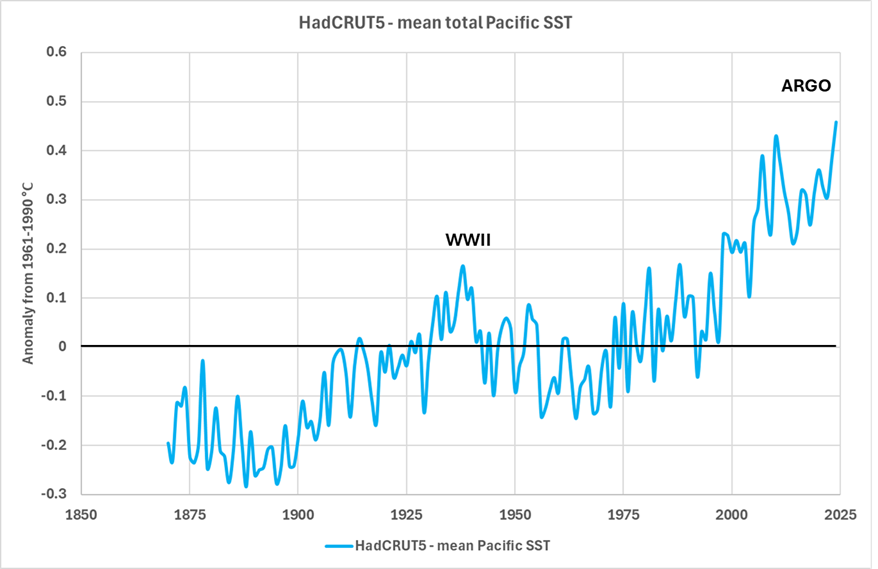
The odd thing about the list in table 2 is that none of them cover the entire Pacific Ocean, although the TPI comes close. An obvious question is how does the mean Pacific SST compare to HadCRUT5? The R2 statistics in Table 1 are useful, but as we have seen in this series it is not enough. The acid test of correlation, especially when dealing with time series, is to examine a graph of the data series being compared. We want to see how trend direction changes compare between series. The calculated, and area-weighted series are shown in figure 1.

It is not surprising that the total Pacific HadSST4 and ERSST5 mean SST records have the best correlation with HadCRUT5. It is a little surprising that the ERSST5 AMO, covering only one-fourth the area of the Pacific, does so well and nearly as well as the North Pacific alone (16% of Earth).
But we need to examine the graph in figure 1 more closely, the devil is in the details. All the anomalies in figure 1 are from their respective mean values from 1961-1990. Thus, they closely agree in that period. I find it suspicious that HadCRUT5 is the second highest value from around 1998 to 2024 as well as the lowest value from 1850 to 1905. It only joins the remaining means from 1905 to the mid-1990s.
It is true that land warms and cools faster than water due to its lower heat capacity, but land only occupies 29% of Earth’s surface, less than the area covered by the Pacific. Should this affect the HadCRUT5 trend over periods as long as 1998-2024 and 1850-1905? The fact that the difference is negative in the 19th century and positive in the 21st is suspicious, and a little too convenient for the “consensus” by far.
The Pacific is the world’s largest ocean, and one would think it has a huge influence on the HadCRUT5 global mean surface temperature (GMST), but if so, it isn’t clear in figure 1. It also isn’t clear in the commonly cited oscillations and indices listed in table 2 or any other Pacific oscillation. All I see, from a global perspective, when I look at the Pacific oscillations is a confusing mess. They are very important regionally, less so globally. More on this in later posts. These oscillations have a significant impact on North & South American weather and weather in the Far East, but they do not correlate with HadCRUT5 very well.
Could HadCRUT5 be the problem? HadCRUT5 is virtually identical to the BEST global average surface temperature record (Rohde & Hausfather, 2020) relied upon a lot in AR6. HadCRUT5 is also similar to other records of estimated global surface temperature, so we don’t think it is a simple error in data gathering, but it could be due to errors in processing and “correcting” the data as discussed here. Figure 2 shows how the mean total Pacific SST correlates with HadCRUT5.


Figure 2 compares the mean total Pacific SST from HadSST, HadISST, and ERSST to HadCRUT5. Figure 3 plots the difference between HadCRUT5 and the mean Pacific SST. The largest positive difference (HadCRUT5 larger than the Pacific mean) occurs from 2000 to the present and the largest negative difference occurs in the 19th century, which has the result of inflating the global surface warming rate.
Surprisingly the largest standard deviation of the total Pacific mean SST since 1941 occurs during the modern era when we have ARGO float data, which are the highest quality SST measurements. The only period of comparable standard deviations is from 1870 to World War I when SST measurements were very sparse and of low quality. There is one spike in 1941 that is as bad as the peak in 2022, but otherwise every yearly standard deviation since 1923 is below the values since 2016, very odd.
This makes little sense, the equipment used from 2016 to today is the best that has ever been deployed, further the modern era has satellite temperature measurements, which were unknown before 1978. It is well known that the worst period for SST data is during World War II (WWII), yet the standard deviation is minimal in that period. Why should HadCRUT5 and the total Pacific mean SSTs agree best during World War II? The collected data was awful then, it can only mean the three reconstructions (HadISST, HadSST, and ERSST) used the same methods to deal with the bad data in WWII, it cannot mean the estimates are more accurate.
Many will remember figure 4, which compares HadCRUT3, 4, and 5. This illustration first appeared when HadCRUT5 first came out and it illustrates how different processing methods have increased the global average surface temperature for nearly every year from 2000 to 2014. The data used by the Hadley Centre didn’t change between 2000 and 2014, only the processing and “error corrections.”

Figures 2 to 4 show that the warming rate from HadCRUT5 is very suspect. It also shows that modern estimates of SST are probably getting worse as the data is getting better. It is highly unlikely that three different estimates of Pacific mean SST would be more different since 2005 when data from thousands of highly accurate Argo floats became available. It is also dubious that the modern era is less accurate than the World War II period when the data was awful. Something is wrong.
Discussion
As figures 2 and 3 make clear, most of the time from around 1910 through 1975, the total Pacific mean SST anomaly, and its standard deviation track well with HadCRUT5. Before 1910 and after 1975 HadCRUT5 is outside the Pacific mean standard deviation and before 1910 it is below the Pacific mean temperature and after 1975 it is above. I suppose that there could be some climate influence causing this, but it seems unlikely. Considering the huge heat capacity in the Pacific, relative to the global atmosphere, the difference in warming trends between the Pacific and the global surface for these multidecadal periods is not credible.
As I discussed and documented here, the World War II period was a period of great error in SST data, both because of the war itself and because of the transition from measuring SST in insulated buckets dipped into the ocean to measuring it with instruments in ships’ engine cooling water intake ports. This should be the period when different estimates of mean total Pacific SST are maximally different, not minimally different.
The modern era, when we have Argo floats and abundant tethered ocean buoys, should have the best data and the least uncertainty, but figures 2 and 3 show the opposite. The whole issue of how well or how poorly SST is estimated is discussed in more detail here. It seems likely that there is a problem with the HadCRUT5 reconstruction of global surface temperature. There are also problems with estimating Pacific mean temperature, but why should the comparisons in figures 2 through 4 indicate that the error in these estimates is increasing? It seems very odd.
Useful references related to this post are listed below, See here and here for more information on the topics discussed and the references below. In the next post I will discuss the North Pacific Index (NPI), as originally planned.
References
Brönnimann, S. (2003). A historical upper air-data set for the 1939–44 period. International Journal of Climatology, 23(7), 769-791. doi:10.1002/joc.914
Brönnimann, S., & Luterbacher, J. (2004b). Reconstructing Northern Hemisphere upper-level fields during World War II. Climate Dynamics, 22, 499-510. doi:10.1007/s00382-004-0391-3
Brönnimann, S., Luterbacher, J., & Staehelin, J. (2004). Extreme climate of the global troposphere and stratosphere in 1940–42 related to El Niño. Nature, 431, 971–974. doi:10.1038/nature02982
Freeman, E., Woodruff, S., Worley, S., Lubker, S., Kent, E., Angel, W., . . . Smith, S. (2017). ICOADS Release 3.0: a major update to the historical marine climate record. Int. J. Climatol., 37, 2211-2232. doi:10.1002/joc.4775
Hegerl, G. C., Brönnimann, S., Schurer, A., & Cowan, T. (2018). The early 20th century warming: Anomalies, causes, and consequences. WIREs Climate Change, 9(4). doi:10.1002/wcc.522
Huang, B., Thorne, P. W., Banzon, V. F., Boyer, T., Chepurin, G., Lawrimore, J. H., . . . Zhang, H.-M. (2017). Extended Reconstructed Sea Surface Temperature, Version 5 (ERSSTv5): Upgrades, Validations, and Intercomparisons. Journal of Climate, 30(20). doi:10.1175/JCLI-D-16-0836.1
IPCC. (2021). Climate Change 2021: The Physical Science Basis. In V. Masson-Delmotte, P. Zhai, A. Pirani, S. L. Connors, C. Péan, S. Berger, . . . B. Zhou (Ed.)., WG1. Retrieved from https://www.ipcc.ch/report/ar6/wg1/
Kennedy, J. J., Rayner, N. A., Smith, R. O., Parker, D. E., & Saunby, M. (2011). Reassessing biases and other uncertainties in sea surface temperature observations measured in situ since 1850; 1. Measurement and sampling uncertainties. Journal of Geophysical Research, 116. Retrieved from https://agupubs.onlinelibrary.wiley.com/doi/full/10.1029/2010JD015218
Kennedy, J. J., Rayner, N. A., Smith, R. O., Parker, D. E., & Saunby, M. (2011b). Reassessing biases and other uncertainties in sea surface temperature observations measured in situ since 1850: 2. Biases and homogenization. J. Geophys. Res., 116. doi:10.1029/2010JD015220
Kennedy, J., Rayner, N. A., Atkinson, C. P., & Killick, R. E. (2019). An ensemble data set of sea-surface temperature change from 1850: the Met Office Hadley Centre HadSST.4.0.0.0 data set. JGR Atmospheres, 124(14). Retrieved from https://agupubs.onlinelibrary.wiley.com/doi/abs/10.1029/2018JD029867
Lluch-Belda, D., Crawford, R. J., Kawasaki, T., MacCall, A. D., Parrish, R. H., Schwartzlose, R. A., & Smith, P. E. (1989). World-wide fluctuations of sardine and anchovy stocks: the regime problem. South African Journal of Marine Science, 8(1), 195-205. doi:10.2989/02577618909504561
Mantua, N. J., Hare, S. R., Zhang, Y., Wallace, J. M., & Francis, R. C. (1997). A Pacific Interdecadal Climate Oscillation with Impacts on Salmon Production. Bull. Amer. Meteor. Soc, 78, 1069-1080. Retrieved from https://journals.ametsoc.org/view/journals/bams/78/6/1520-0477_1997_078_1069_apicow_2_0_co_2.xml
Rayner, N. A., Brohan, P., Parker, D. E., Folland, C. K., Kennedy, J. J., Vanicek, M., . . . Tett, S. F. (2006). Improved Analyses of Changes and Uncertainties in Sea Surface Temperature Measured In Situ since the Mid-Nineteenth Century: The HadSST2 Dataset. J. Climate, 19, 446-469. doi:10.1175/JCLI3637.1
Rohde, R. A., & Hausfather, Z. (2020). The Berkeley Earth Land/Ocean Temperature Record. Earth System Science Data, 12(4). doi:10.5194/essd-12-3469-2020
Trenberth, K., & Hurrel, J. (1994). Decadal atmosphere-ocean variations in the Pacific. Climate Dynamics, 9, 303-319. doi:10.1007/BF00204745
Why are we accepting the margins of error from 80-120 years ago? I’m thinking a bucket of the side by a 17yo swabbie in WWII might not have the resolution of a recent climate researcher.
In a field where people fuss about every 0.1 of a degree change, I’m amazed at how poorly the data holds together. Referring to figure 2, the linear least squares warming rate for the Mean Pacific SST line is 0.46 deg/century.
The linear least squares slope for HadCRUT5 is 0.7 deg/century.
These are big differences, probably too big to be natural.
How can we be obsessed with global warming when we cannot measure it any more accurately than that? It is pointless to use a micrometer to measure a brick.
___________________________________________
Nice one! And not exactly the same as:
Trying to measure Jello® with a rubber yard stick
The PROBITY and PROVENANCE of all climate metrics are seriously lacking, and not fit for adopted purposes.
Watch this video. It reviews the Hockeystick. It is a complete joke.
https://app.screencast.com/nXfZcUyGR4QlR
The author is ‘Anonymous’. And that’s your go-to authority?
Can you counter a single thing in the video?
Yes, it’s complete nonsense based on the flawed belief that 15μm radiation is only emitted by material at -80ºC!
Could it be something to do with the infamous, probably highly contrived pausebuster paper, that Obama probably demanded to secure the Paris agreement during an inconvenient long period of no global warming?
If it erased a pause that was really there, goodness knows what distortions it would create going forward. Rest is Google AI:-
The paper, “Possible artifacts of data biases in the recent global surface warming hiatus” by Karl et al. (2015), published in Science, addressed the apparent slowdown in global surface warming observed in the late 20th and early 21st centuries, often referred to as the “pause” or “hiatus”. The study concluded that the hiatus was largely an artifact of data biases and that warming had continued at a rate comparable to the latter half of the 20th century. The paper primarily focused on updating the ocean temperature record and found that including previously overlooked data, particularly from buoys, revealed a more consistent warming trend.
HadCRUT, specifically HadCRUT4, began incorporating aspects of the Karl et al. (2015) revised sea surface temperature (SST) data in 2015, though not directly as a complete replacement. The changes were introduced in a phased manner, with some adjustments first appearing in HadSST3 and then later in HadCRUT4.
Thus, the phrase “Karlizing the data” appeared.
Make me think Karamelizing the data would be an improvement, perhaps.
Sounds sweeter, easier on the taste buds
I was immediately struck by the disagreement between the ARGO-era SST data and the other sources, as shown in Fig. 2.
I think that the important point here is that, as I recollect, Karl adjusted the ARGO data to agree with boiler room intake temperatures, which were known to be inferior to the ARGO data. Since when does any honest scientist make systematic adjustments that make high-quality data agree with poor-quality data?
There was also an issue about some of the temperature sensors used by ARGO buoys, whose details I have forgotten.
“The paper primarily focused on updating the ocean temperature record and found that including previously overlooked data, particularly from buoys, revealed a more consistent warming trend.”
Each part of that sentence raises so many questions.
Why was the previous data overlooked?
On what ways are buoy measurements different?
Revealed or created?
The 19th plus 20th century was a period of great error in SST data.
Agreed, and that is 71% of the surface of the Earth! But the 1940s stand out, it was not only a huge El Nino period, but the data is awful. We really didn’t see decent data until after 2005, and yet the Karlized reconstructions try and paint the last 20 years as bad. Totally illogical.
If Pat Frank’s paper were correct, how do we explain the strong agreement between satellite and surface temperature records? These datasets are independent. Satellites measure tropospheric temperatures from space, while surface datasets rely on direct ground and ocean observations. Yet the long term warming rates differ by at most 0.1C per decade. If the uncertainty were as large as Frank claims, we’d expect far greater divergence.
Commenter Bellman calculated a correlation coefficient of 0.83 between UAH version 6 and the GISS surface temperature record. His graph is attached.
Also, both satellite and surface datasets clearly resolve ENSO cycles, which show up as distinct, coherent patterns in the temperature record. If the uncertainty really drowned out meaningful signal, we wouldn’t be able to track ENSO this reliably.
The graph is not attaching.
I don’t need to see the graph, the R^2 is not the meaningful statistic here. You need to compare the respective rates of warming which I’ve done below.
They do warm together and cool together, which is what R^2 will tell you, the problem is the slopes over 40 years don’t match. You need to look at the right thing.
Janet,
What agreement?? As you can see in the attached graph, UAH has a linear least squares slope of 0.14 deg/decade and HadCRUT5 has a trend of 0.19 deg/decade. This is a difference of over 30%. Further this is only since 1978, the end of a cool period, everything is increasing since 1978, it is a poor period to compare trends, yet HadCRUT5 still fails.
A 0.05 C/decade difference in long term trend between UAH and HadCRUT5 is nowhere near the level of uncertainty Pat is claiming.
Pat argues that the entire instrumental record is so dominated by error propagation that it’s essentially meaningless. If that were true, satellite and surface datasets, entirely independent systems using fundamentally different methods, would diverge wildly, not differ by less than 0.1 °C/decade over nearly half a century.
And the variations between datasets aren’t chaotic or random. They are more consistent than not.
If the uncertainties were truly on the scale Frank suggests, the time series would be a garbled mess: One month would read -0.5 C, the next +0.8 C, and the signal would be buried in noise. Yet we see consistent ENSO patterns and seasonal cycles emerge clearly across all datasets.
Also consider CERES satellite data, which measures absorbed shortwave radiation, completely independent from surface temperature measurements.
As a shown in Figure 7 of this paper, the absorbed solar flux and global surface temperature anomalies are highly correlated with a consistent 0–9 month lag. That’s a physical relationship, not a coincidence.
https://www.mdpi.com/2673-7418/4/3/17
When considering the consistency across independent lines of evidence, it is really hard to believe that the massive uncertainty bars Pat alleges are accurate.
You need to go back to school. An uncertainty interval tells you nothing about accuracy. It tells you an interval wherein you have no way to discern what the true value actually is.
USCRN has an uncertainty of ±0.3°C. That doesn’t mean the point value (center of the interval is the true value. It means that you have no way to know where the actual true value lays within that interval.
R² values calculated using point values of an uncertainty interval only assumes that each and every point value are 100% accurate. To truly analyze the difference, one must assess each and every possible combination of possible values inside the uncertainty interval. Different combinations will result in different slopes of regression trends. Only then can one see how well the trends actually match.
From 1979/01 to 2024/12 the trend is
+0.152 ± 0.043 C.decade-1 for UAH v6.1.
+0.203 ± 0.025 C.decade-1 for HadCRUT v5.0.2.
The trend PDFs have mutual overlap. One can thus reasonably argue that they are consistent with each other at least in the range 0.178 – 0.195 C.decade-1.
It is worth pointing out that UAH and HadCRUT measure different things so there is no expectation that they should be exactly the same anyway.
In particular, the specific heat capacity of water is about 4X that of air (for equal weights) meaning that the range in temperature of water should be about 1/4th that of air. Also, since it takes 4X as much energy to heat the same weight of water, one can expect a small lag in the peak temperature of the water.
In the first place, correlation does not indicate accuracy.
In the second, agreement between the surface and satellite records should be a matter of suspicion, not of support.
Suspicion is the only analytically proper regard in light of the unambiguous and large measurement errors field calibration experiments have invariably revealed, coupled with the specious adjustments Andy has demonstrated here.
The linked LiG Met paper ends this way, “Very evidently, a professionally competent and disinterested third party must be commissioned to produce a full and rigorous instrumental engineering evaluation of the historical temperature record. It is here recommended that the American Society for Precision Engineering constitutes one such independent and competent third party. Along with precision engineering societies from other countries, their full, independently replicated, and delivered evaluations of meteorological air temperatures must precede any further actions.”
No one can legitimately object to that undertaking.
The program should be government-funded, there should be several independent non-communicating teams, and include absolutely no interested parties; none by participation, nor for advice, nor for review.
The whole argument about surface air temperature would be resolved in a year – perhaps two.
The program should have been done 40 years ago.
I object on the basis that “a professionally competent and disinterested third party” can’t survive agree-with-the-person-signing-my-check bias for long enough “to produce a full and rigorous instrumental engineering evaluation of the historical temperature record.“
Roy Spencer, who operates UAH, is about as disinterested as it gets. That alone should make you pause before claiming that agreement is somehow suspicious.
in the first place, an argument from authority is no argument.
In the second, Roy shrugged off the (+/-)0.3 C resolution of the satellite radiometers, when I asked him about it. It should condition the UAH temps, but he ignores it.
In the third, Roy’s criticism of Propagation, posted right here at WUWT was an embarrassment of incompetence. He showed no understanding or appreciation of physical uncertainty or how to evaluate it.
In the fourth, you passed over in silence the copious evidence from field calibrations that surface air temperature measurements are riven with systematic error.
Look Janet, you can be a scientist and argue rigor or you can be a advocate defending a narrative.
But don’t pretend the former while doing the latter.
I’ve already explained this: in climate science, what matters are relative changes over time, not absolute accuracy. For that, you only need precise averages, not perfectly calibrated absolute values.
If there’s a fixed systematic error, anomalies allevaite it. If the error varies over time, homogenization addresses it. Look at the USCRN. It was designed to avoid many of the biases critics cite, yet it aligns closely with the adjusted temperature record.
For more detail on how averaging improves precision, I recommend this article. It’s quite conclusive:
https://moyhu.blogspot.com/2016/04/averaging-temperature-data-improves.html#more
With respect, you’re not in a position to accuse me of defending a narrative when you’re the one suggesting there’s something suspicious going on, something that would apparently implicate even Roy Spencer of all people.
Finally, see my reply to Andy at 2:26 PM. Ask yourself this: if the surface temperature record were riddled with major error bars, why is there so much independent verification supporting it?
Nick Stokes’ LLN solution requires perfect rounding. However, limited resolution itself obviates that possibility. Systematic measurement errors guarantee incorrect rounding.
The means will be wrong. The normals will be wrong, The anomalies will be wrong. But no one knows by how much. Hence the uncertainty bounds.
You wrote, “If the error varies over time, homogenization addresses it.” An assumption undemonstrated.
The Figure shows temperature trends measured using a sonic anemometer (unaffected by wind or insolation) or a PRT in a naturally ventilated gill shield.
The PRT anomalies show a false warming trend. Nevertheless, the trends are highly correlated.
No statistical homogenization test will detect the wrong trend.
The published field calibrations are unambiguous. As an experimental scientist, I must accept them.
If the published record doesn’t reflect known uncertainties, it merits a skeptical reception. Not helped when those in the field invariably misrepresent the measurement errors as random.
My comments about Roy are from direct experience and a full analysis of his criticism.
Wrong. It has been demonstrated.
Look at USCRN and compare it to the adjusted historical network. Despite different instrumentation and vastly improved accuracy, their trends align remarkably well. That convergence is empirical validation.
Your PRT anomalies are clearly just one limited setup.
Focusing all your effort on discrediting one dataset while ignoring the rest is like cutting off one head of an eight headed dragon and declaring victory. The others are still standing, just as strong, all pointing in the same direction.
Then why aren’t the anomalies incoherent? Why do known climate phenomena like ENSO and volcanic eruptions emerge clearly across datasets, despite being measured through entirely different systems?
1) “That convergence is empirical validation.”
Or a consequence of tendentious adjustments.
Back when leaked ClimateGate emails revealed consensus shenanigans, Willis Escehnbach did a dive into HCN adjustments, with a particularly deep dive into the record at Darwin, Australia.
His conclusion: “They’ve just added a huge artificial totally imaginary trend to the last half of the raw data! …Those, dear friends, are the clumsy fingerprints of someone messing with the data Egyptian style … they are indisputable evidence that the “homogenized” data has been changed to fit someone’s preconceptions about whether the earth is warming.”
Jennifer Marohasy has been investigating falsified Australian temperature records, for years. Not to mention her exposure — and Peter Ridd’s — of the lies about the imminent death of the Great Barrier Reef.
2) “Your PRT anomalies are clearly just one limited setup.”
The PRT result shows the same sort of bias that every single published field calibration reveals.
The general conclusion is that sensors housed in a naturally ventilated shield produce wrong temperatures.
This problem was known and discussed in the 19th century. But today it’s ignored.
3) “Focusing all your effort on discrediting one dataset …”
You didn’t read Lig Met, did you. Many field calibrations are discussed. The PRT trend was a convenient example of a general finding. I didn’t discredit it. I reported it.
4) “Then why aren’t the anomalies incoherent?”
Because data contaminated with systematic error behaves exactly like good data.
The PRT trend is a good example, Without the sonic anemometer comparison, the PRT trend would be accepted as correct. It would pass all the tests of homogeneity.
This truth is why an independent calibration standard is needed. Without one, the measurement errors are invisible.
5) “phenomena like ENSO and volcanic eruptions emerge clearly across datasets”
They’re the product of the standard instruments. Why wouldn’t they all register large-scale perturbations?
Instruments putting variable systematic error into measurements will be self-consistent.
The bounds I show are uncertainty, not error. Uncertainty means the instruments are unreliable.
We never know the true temperatures. We only know the measurement and the calibration bounds of the instrument.
One can make a leap of faith and decide the readings are perfectly reliable even though the instruments are not. But then one is no longer doing science or being a scientist.
Nick Stokes wrote a post about this at the time:
https://moyhu.blogspot.com/2009/12/darwin-and-ghcn-adjustments-willis.html
The adjustment was triggered by a documented metadata change. As Nick has demonstrated, homogenization algorithms can produce both cooling and warming adjustments. They respond to discontinuities, as they’re designed to do. On a global scale, the net effect is minimal. There’s no grand conspiracy here.
https://moyhu.blogspot.com/2015/02/homogenisation-makes-little-difference.html
https://moyhu.blogspot.com/2015/02/breakdown-of-effects-of-ghcn-adjustments.html
My understanding is that homogenization has limitations in data sparse regions. It works well in regions with lots more data. But this is all different from your allegations about instrument error.
I read it carefully and did my best to engage with it in good faith. My point was about the independence of multiple datasets and metrics, not about inter-comparisons from specific field calibration experiments.
If this error you’re describing were truly widespread, it would introduce a clear, spurious trend in a noisy global average. But we have substantial evidence showing that hasn’t happened. You’ve cast doubt on satellites.
How do you explain the consistent 9 month lag between CERES-measured solar radiation flux and global temperature? I shared that with Andy above.
What about sea level rise slightly decelerating from WWII through the 1970s, matching the mid century cooling shown in the surface temperature record? Another coincidence?
Are you really going to convince yourself that all of these independent metrics are wrong, and all in mostly the same direction and magnitude? How do you hold that view without running into cognitive dissonance? I’m really asking!
Nobody thinks that. Scientists know that they are not perfectly readable. They express confidence but absolute certainty.
But when one doesn’t work with uniformly or randomly sampled data, it introduces a problem of weighting the data and having more influence from over-sampled regions.
What does ‘randomly sampled’ mean? Homogenization doesn’t works with data that is randomly sampled. It incorporates data from nearby stations to improve the consistency of the target station’s record.
“to improve the consistency of the target station’s record.”
Making the target station’s data no longer independent. There’s no longer any point to include it in the average.
Homogenization doesn’t work well with intensive values at all.
How do you set the temperature at a mountain peak equal to the average of a measurement station on the east side of a mountain and a measurement station on the west side of the mountain. They each get different insolation at different times and who knows what the wind does.
How do you “homogenize” the temperature of a station down in a valley with one high on a plateau to get the temperature in between the two? Even if they are only 20 miles apart?
That is exactly why scientists use temperature anomalies rather than absolute temperatures. Anomalies track deviations from each station’s own long term average, so even if the east and west sides have different base temperatures, they tend to warm or cool in parallel relative to their own baselines. That shared signal is what allows us to compare and aggregate across varied terrain. That also allows for homogenization, if needed.
“That is exactly why scientists use temperature anomalies rather than absolute temperatures. Anomalies track deviations from each station’s own long term average”
More climate science garbage. If the long term average is inaccurate then how can the anomaly be accurate?
You are applying the common misconception in climate science that “all measurement uncertainty is random, Gaussian, and cancels”. Leaving the stated values as 100% accurate.
If I give you 100 temperature measurements, each with a measurement uncertainty of +/- 1.8F what is the measurement uncertainty of the average? (hint: it ain’t +/- 1.8F, it isn’t even less than +/- 1.8F).
“[Homogenization] works well in regions with lots more data.”
Homogenization adjusts data to be more uniform. The notion that it makes data more accurate is an assumption.
“your allegations about instrument error.”
I don’t make allegations about instrumental error. I report the results of field calibrations, which invariably reveal instrumental error.
“If this error you’re describing were truly widespread, it would introduce a clear, spurious trend in a noisy global average.”
Your spurious trend would not be clear, because it would be the data itself. Measurement error is undetectable without an external accuracy standard.
“the independence of multiple datasets and metrics,”
They all use the same data. The satellite data are independent, But that dates only from 1979. And RSS adjustments have been changed to make the satellite record closer to the surface record.
Radiometer resolution is never included in the satellite record. That is a failure.
“How do you explain the consistent 9 month lag between CERES-measured solar radiation flux and global temperature? I shared that with Andy above.”
Naturally ventilated sensors will respond to perturbations. But the measured temperatures will be variably incorrect. And no one will know by how much.
The question concerns knowledge of accuracy, Janet. When the instruments are categorically known to produce incorrect measurements, an uncertainty metric must be applied to the values.
“Are you really going to convince yourself that all of these independent metrics are wrong, and all in mostly the same direction and magnitude? How do you hold that view without running into cognitive dissonance? I’m really asking!”
Your metrics do not bear on accuracy, but on general trends.
Your argument is circular. You are citing results known to be the compilation of poor data (“independent metrics“), to support the validity of the poor data.
Data with systematic errors will behave systematically. Systematic behavior is no proof of accuracy.
My view is that naturally ventilated sensors produce inaccurate air temperatures. This is a demonstrated fact and therefore ineluctable. The uncertainty in result necessarily follows. Understand: the uncertainty necessarily follows. Your metrics are irrelevant to that fact.
“Nobody thinks that.”
They all think that, Workers in the field assume all measurement error is random and averages to near zero. Even SST. The minuscule uncertainties they provide are tantamount to a claim of perfect accuracy. The protocol is wildly deficient and the practice is ludicrous.
The whole field calls for a deep and independent third party investigation to iron it all out.
Here we go again. You just claimed that the USCRN aligning with the adjusted record is just a coincidence and that homogenization is less effective outside the U.S. But you’ve avoided addressing the more likely explanation: the reduced accuracy elsewhere is due to sparse station coverage, not instrument error. The fact that you’re repeating the same assertion without engaging with this point is telling.
Except the previous RSS version was more consistent with the current UAH data, which, as both I and bdgwx pointed out earlier, does not support your uncertainty estimate. I remember when Chris Monckton used RSS for his ‘pause’ articles. Once the adjustment was made, though, RSS was abandoned, and the ‘skeptics’ quickly jumped ship.
How much would the final average be affected if your raw numbers were off by +/- 0.3°C? If the difference is small, what does that say about the significance or resolution of the error?
Well, this is awkward because this is inconsistent with what your paper concludes:
“However, at the 95% level of uncertainty, neither the rate nor the magnitude of 19th or 20th century warming can be known.”
Given what you’ve said, what exactly is the significance of your uncertainty estimates? Climate science is primarily concerned with trends over time, and since you’ve conceded that those trends are largely unaffected, is there much to question regarding the validity of the data?
While achieving absolute instrumental accuracy is difficult, that doesn’t mean we can’t measure large-scale changes in weather over time. You mentioned that above.
“You just claimed that the USCRN aligning with the adjusted record is just a coincidence and that homogenization is less effective outside the U.S.”
I claimed neither of those things.
“does not support your uncertainty estimate.”
Uncertainty is not error.
Land surface temps are measured at ~5.5 feet. SSTs sample variable depths..The lower troposphere satellite temps are the average radiance of the thick atmospheric layer of zero to 7 km.
Why would anyone think it should reproduce the surface record?
In any case, the uncertainty analysis stands on its own merits. It assesses published field calibrations — both land station and SSTs. The measurement uncertainties are a fact.
You and bdgwx use a hand-waving comparative argument to dismiss. The counter is that the correspondence of surface and satellite records is a matter of suspicion, given the known inaccuracies of the surface measurements.
“How much would the final average be affected if your raw numbers were off by +/- 0.3°C?”
That’s not the meaning of uncertainty It’s not that they’re off by (+/-)0.3 C. It’s that they’re not known to better than (+/-)0.3 C.
“Well, this is awkward because this is inconsistent with what your paper concludes:
“However, at the 95% level of uncertainty, neither the rate nor the magnitude of 19th or 20th century warming can be known.””
That conclusion is not vitiated by your metrics.
The 20th century began in 1901. The satellite record began in 1979. What was the rate or magnitude of change between 1901 and 1979? No one knows.
And the satellite record tells us the mean temperature at ~3.5 km, which is not the surface and is ~21 C colder than the surface.
“and since you’ve conceded that those trends are largely unaffected, is there much to question regarding the validity of the data?”
My point was your trends are irrelevant to an uncertainty metric. The trends are conditioned by their measurement uncertainty bounds.
The trends are associated with a large measurement uncertainty. This means one has no idea of the physically correct trend, or the relationship between the known trend and the correct trend.
“While achieving absolute instrumental accuracy is difficult, that doesn’t mean we can’t measure large-scale changes in weather over time. You mentioned that above”
I mentioned that inaccurate sensors will respond to perturbations. That doesn’t mean they respond accurately.
It means that whatever large scale changes one observes — and we’re talking about 1 C = large scale — one has no idea whether the measured changes are the physically true changes. Only that the true changes lay somewhere within the measurement uncertainty bounds.
You are right. I did mistakenly attribute that specific claim to you. You actually said the adjusted data is “a consequence of tendentious adjustments,” and I apologize for the misattribution. That said, it is not. And you’re still sidestepping the point that the reduced effectiveness of homogenization in certain areas has nothing to do with instrument error.
Those specific details are not directly relevant. The primary objective is to measure how weather varies over time relative to a consistent baseline. The exact value of that baseline doesn’t need to be perfectly accurate, because the deviations from the long term average remain the same regardless. This makes the baseline a useful mathematical reference point that helps address the concern you’re raising.
The variations are large enough that small uncertainties, like +/- 0.3C, become negligible. This is why the global average temperature variations and trends are so consistent and reproducible. Those are the key signals. The same principle likely applies to the other datasets and metrics I’ve mentioned.
It is clear that the approach works. Yes, we can’t measure absolute real world temperatures without field calibration but we can see how closely the temperature data used in climate science aligns with the real world by comparing the trends in other physical metrics:
Sea level rise: Slows from the 1940s to the 1970s, then accelerates in the 1990s, which aligns well with the surface temperature record.
CERES solar radiation flux: Shows a lead of 0-9 months relative to surface temperature changes. A known physical relationship between solar radiation and temperature!
Those are “physically true” metrics (your word).
The odds of those datasets aligning are astronomically low, making your assertion “You are citing results known to be the compilation of poor data (‘independent metrics’) to support the validity of the poor data” incredibly implausible.
Your argument also hinges on the notion that the adjustments were somehow reverse engineered to mimic CRN just enough to appear legitimate to the public, while secretly inflating warming.
That’s a claim with no compelling evidence.
When you pair that with the statistical unlikelihood I outlined above, it’s clear that measurement uncertainty isn’t a legitimate problem. It’s making a mountain out of a molehill, and a mathematically indefensible one at that.
“That said, it is not.”
How do you account for the attached graphic showing systematic modifications of the past GISS record?
“And you’re still sidestepping the point that the reduced effectiveness of homogenization in certain areas has nothing to do with instrument error.”
That was never my point, either.
The central issue is that one never knows the physically true temperature. One is left only with calibration uncertainty to condition field results.
“The exact value of that baseline doesn’t need to be perfectly accurate, because the deviations from the long term average remain the same regardless.”
You’re assuming – with zero justification – that measurement error is a constant offset. And constant over decades to boot. Taking anomalies is not known to remove error. It *is* known to increase uncertainty.
“Yes, we can’t measure absolute real world temperatures without field calibration…”
The point is one doesn’t know real world temperatures because the sensors produce poor data. And have certainly done over the historical record. It is impossible to correct past data burdened unknown systematic error.
“[sea level rise] which aligns well with the surface temperature record.”
Correlation is not causation. And you imply sea level rise is due to increased SST. But measurement of SST is of very poor quality. It cannot support assignment of cause.
“A known physical relationship between solar radiation and temperature!”
There exists no physical theory of the climate that can predict an irradiance-air temperature relationship to the level of detail you require.
“The odds of those datasets aligning are astronomically low,…”
A physically unjustified pseudo-statistical inference. There’s no way to calculate such odds.
“[Tendentious adjustments are] a claim with no compelling evidence.”
See the posted graphic. Look into the Climategate emails about tweaking the SST record to remove the 1940’s warm blip. See Tony Heller’s plot of temperature adjustments vs. CO2 rise.
“measurement uncertainty isn’t a legitimate problem.”
Measurement error conditions the global record with (+/-)1.9 C uncertainty.
You’ve argued against the uncertainties demonstrated in LiG Met without producing a word of criticism of the analysis itself. You’ve merely tried to wish it away with hand-waving arguments about correlation.
“It’s making a mountain out of a molehill,...”
Rather, you defend the making of a silk purse from a sow’s ear.
“...and a mathematically indefensible one at that.”
A dismissal you cannot support in evidence.
“Measurement error conditions the global record with (+/-)1.9 C uncertainty.”
That is a *MINIMUM* value. It is quite likely larger than this.
You’re right. It’s close to the lower limit of uncertainty.
Where is the source for this graph?
I never assumed that. I specifically said that time varying systematic errors can be addressed through homogenization. You’ve been pushing back with conspiracy theories propped up by a discredited 2009 WUWT blog post, cherry picked excerpts from the Climategate emails, Tony Heller’s usual distortions, and now an unsourced image. IOW, a collage of misinformation.
We may not be able to perfectly correct the absolute values, but we can reliably estimate anomalies relative to a fixed baseline, and those anomalies show strong correlations over distances up to 1000 km.
Earth’s average temperature is governed by energy balance. When absorbed solar radiation equals outgoing infrared radiation, Earth is in thermal equilibrium and its temperature stays steady. But if the incoming solar flux exceeds outgoing radiation (after accounting for albedo), Earth retains more energy, leading to a positive energy imbalance and warming. This is proven physics.
As the Earth warms, the cryosphere melts, releasing more meltwater into the oceans and raising sea levels.
The observed alignment between rising global temperatures and accelerating sea level rise isn’t a spurious correlation. It reflects a direct physical relationship.
Been there, done that. The so-called “1940s warm blip” has been addressed thoroughly. This wasn’t some hidden manipulation. It was a known issue long before Climategate, which is exactly why that scandal was nonsense from the start.
The controversy was seized on by the uninformed, but the context was already public. For example, this RealClimate post from June 2008, before the email leak, breaks it down clearly:
https://www.realclimate.org/index.php/archives/2008/06/of-buckets-and-blogs/
Tony Heller’s criticisms about temperature adjustments and the correlation with CO2 trends are based almost entirely on U.S.-specific data, and not global.
The early 20th-century downward adjustment in U.S. temperature data that Steve Goddard uses is primarily due to corrections for TOBs.
Even Anthony Watts acknowledged the correction and used the TOBs-adjusted version in his 2011 study.
I don’t have much experience with metrology, Pat, so I have to evaluate your claims using other lines of reasoning.
Judging by your responses, broad independent agreement seems to be a major problem for your argument.
You’ve tried to dismiss the physics behind EEI by suggesting we can’t understand the relationship between solar radiation and temperature without a full “physical theory of climate”.
Likewise, your claim that the alignment between global surface temperature and sea level rise is just a correlation, and not causation, ignores well established physical mechanisms linking the two.
On top of that, the sources you cite to support your argument about temperature adjustments being intentional manipulations come from widely debunked misinformation.
“ I specifically said that time varying systematic errors can be addressed through homogenization.”
How? If you don’t know the systematic uncertainties in the measurements used for homogenization then how do you know you aren’t just spreading systematic uncertainties around to other locations that would be worse than having no data at all?
The entire point of homogenization seems to be to avoid having empty data slots? So what? If you have 999 temperature data measurements vs 1000 and it makes a significant difference in your average and/or standard deviation of the population then your data is garbage anyway and is not fit for purpose.
It’s the same issue with “adjusting” past temperature measurements to create “long” data sets. Why? If you have 300 long data sets from 1920 to 1930 and 299 long data sets from 1930 to 1940 why go back and adjust anything? If your averages and standard deviations aren’t the same within measurement uncertainty intervals for both time frames then the data is garbage to begin with!
Unless you have a time machine and a calibration lab you can carry back with you exactly how do you determine what adjustment is needed for each measurement?
“We may not be able to perfectly correct the absolute values, but we can reliably estimate anomalies relative to a fixed baseline”
Did you read this before you posted it?
If you don’t know the absolute values accurately then how do you get an accurate baseline? How can an inaccurate baseline result in accurate anomalies?
“Where is the source for this graph?”
I prepared the graphic. I digitized Miles 1978 Figure 1. All the GISS data are online. You can check them yourself.
“I never assumed that [measurement error is a constant offset].”
In this, your statement: “The exact value of that baseline doesn’t need to be perfectly accurate, because the deviations from the long term average remain the same regardless.” you’re assuming error is a constant offset.
“discredited 2009 WUWT blog post,”
Willis’ 2009 post was disputed, not discredited.
“cherry picked excerpts from the Climategate emails”
Right. Commenting on discussion of pruning an embarrassing part out of the SST record is cherry-picking. Look at GISS 1987&1999. Notice anything peculiar around 1940? Coincidence?
“Tony Heller’s usual distortions,”
How do you know his graphic is a distortion?
“but we can reliably estimate anomalies relative to a fixed baseline,”
No, we can’t. And there’s your constant error offset assumption again.
“and those anomalies show strong correlations over distances up to 1000 km.”
LiG Met shows that systematic measurement error strongly correlates between sensors. The errors are due to irradiance and wind-speed – the same physical inputs that determine air temperature. Very likely, therefore, systematic errors will correlate across 1000 km as well. Meaning incorrect anomalies will correlate.
“Earth’s average temperature is governed by energy balance.”
How do you know? Why isn’t it determined by cloud cover? And convection?
“When absorbed solar radiation equals outgoing infrared radiation, Earth is in thermal equilibrium and its temperature stays steady.”
Meaning the Medieval Warm Period, the LIA, the Roman Warm Period, the Minoan Warm Period, the Holocene Climate Optimum and all 7 Glacial-Interglacial periods never happened. Because invariably ASR = OIR and the temperature was always steady.
Your view doesn’t seem to match climate history.
“if the incoming solar flux exceeds outgoing radiation … Earth retains more energy,”
Total incoming solar never exceeds total outgoing IR. Increased CO2 only decreases the IR mean free path. It doesn’t retain energy.
In any case, the TOA radiation balance isn’t known to better than (+/-)3 W/m^2, which is much larger than any purported energy imbalance. Meaning no one knows.
“rising global temperatures and accelerating sea level rise … reflects a direct physical relationship.”
Perhaps. But the warming climate cannot be assigned to a CO2 emissions cause.
“The so-called “1940s warm blip” … has been addressed thoroughly.”
Tendentiously assigned to a 1941-1950 relative decline in bucket vs engine intake SST measurements. One set of temperature numbers corrected with another set of temperature numbers, both of which are of unknown accuracy. Rigorous science indeed.
Heller on TOBS. If you want to dispute that, do so directly with him. Global: You’re right, Heller focuses on the U.S. If the U.S. specifically uses poor ad unusual methods, why have the Brits not called NOAA or GISS out on it.
“Judging by your responses, broad independent agreement seems to be a major problem for your argument”
My adherence to published field calibration experiments is thorough. Therefore the argument is sound.
If there is a broad consensus in opposition, one may legitimately question the consensus methodology. Which I do. It ignores systematic measurement error.
Reiterating, one needs a physical theory of climate to understand the relation of ASR and air temperature. That is not controversial in physics. But the consensus handwaves it away.
“correlation, and not causation, ignores well established physical mechanisms linking the two.”
The point is that SST is so poorly known that any correlation is not uniquely determined. It’s not science-based.
“widely debunked misinformation.”
Debunked means disputed. Not refuted. Misinformation is a label of partisan convenience.
Apart from which, “the sources you cite to support your argument” are published field calibration experiments, none of which are suspect.
My argument is about measurement uncertainty, not adjustments.
I also cite NIST documents, published Joule drift data, and the known non-linearity of the temperature response of LiG thermometers.
All of which play to limits on, or degraded, field accuracy.
And none of which seems to be in your field of view.
“a consistent baseline. The exact value of that baseline doesn’t need to be perfectly accurate, because the deviations from the long term average remain the same regardless.”
You aren’t thinking this through. Deviations don’t *have* to remain the same. In fact, if you don’t know the deviations accurately then how do you know they are consistent?
You are like far too many in climate science in assuming that measurement uncertainty is always random, Gaussian, and cancels. Nothing could be further from the truth. Especially with field measurements taken with non-calibrated instruments.
Why do you think machinists always calibrate their micrometers against a standard gage block before each measurement? Why do you think they always include an uncertainty with their measurement based on the pressure they apply to the instrument heads at each measurement if nothing else? They call the measurement uncertainty “tolerance” but its the exact same thing.
Climate science just blissfully ignores measurement uncertainty. Numbers is just numbers and all measurement uncertainty cancels out!
Because it’s been known since the 1980s that temperature anomalies correlate strongly over distances of up to 1000 km. Scientists know this, which is why they divide Earth’s surface into grid cells.
Because thermometers are used in many applications where high accuracy is needed. Climate monitoring is about detecting relative changes over time.
“Because it’s been known since the 1980s that temperature anomalies correlate strongly over distances of up to 1000 km.”
That’s a typical climate science load of bullcrap. The correlation is seasonal, not daily or monthly. Remove the seasonal time series impact and you get vast differences in the variance of tempeatures.
Compare the temperature measurements of San Diego, CA with Romona, CA, a difference of just 30 miles or so. Vastly different absolute values and variances. Little correlation except for seasonal variation. They both get colder in winter and warmer in summer. Yet both get included with the same weighting in the “global average”.
Don’t like that comparison? Go 30 miles inland from Boston, you’ll find the same exact thing.
Don’t like that one? Compare Boulder, CO with Grand Lake, CO.
Climate science likes to use gridding to equalize spatial representation of data but totally ignores the variances of the temperatures between grids. Supposedly they pick up the variances in the “measurement uncertainty” associated with the global average but have *you* even seen a climate science white paper where that is actually done? I can’t find one that even compares the variance of SH and NH temperatures when one is cold and the other warm! Who cares if they infill grids to get the same number of data points in each if they don’t weight the contributions to the average based on the individual variances!
If the changes over time are subsumed into the measurement uncertainty then how does that help?
If I give you a temperature of 70F +/- 1.8F for Jan 1, 2023 and 70F +/- 1.8F for Jan 1, 2025 what was the actual relative change over time? Did the temperature go up or down over the period?
“ the reduced accuracy elsewhere is due to sparse station coverage, not instrument error. “
The reduced accuracy is from *both*. Instrument uncertainty is endemic in any field measurement, regardless of other measuring sites.
Hubbard and Lin found clear back in 2002 that you cannot adjust temperature readings using regional adjustment factors. Their conclusion was that individual stations require individual adjustments based on calibration with standards. And even those adjustments don’t apply to very far into the past because calibration drift over time is unknown. Part of this has to do with station aging and part with station microenvironment. A station near a corn field will read differently than one near a soybean field vs one near a water impoundment like a pond or lake – even if all three are recently calibrated against a standard.
Trending anomalies means adding the measurement uncertainties of the base *and* the present reading. You can’t just ignore that.
“How much would the final average be affected if your raw numbers were off by +/- 0.3°C?”
This is a MINIMUM measurement uncertainty assessed at the time of manufacture. The actual field measurements can be much less accurate. Even a +/- 0.3C uncertainty legislates against being able to determine anomalies in the hundredths digit. In fact, if you are calculating an anomaly with two values whose measurement uncertainty is +/- 0.3C the measurement uncertainty of the difference is +/- 0.42C. That is very close to being unable to determine the difference in the tenths digit! Microclimate variation can easily push it over the edge making the units digit the proper order of magnitude for the anomaly.
With strong signals, such as eruptions, one can expect them to survive even if they are only qualitatively characterized, such as categorically or ranking. However, if they are not quantitatively measured properly, parametric statistical calculations cannot be trusted, and any conclusions from the statistics will be untrustworthy.
Give an example of a conclusion that becomes unreliable when analyzing volcanic signals in GSAT due to measurement error.
What a joke. This is an invalid EXCUSE that allows climate science to ignore the uncertainty that anomalies inherit from the random variables used to calculate it.
First year statistics students learn that:
when E(X) ± E(Y) = E(X±Y),
Var(X±Y) = Var(X) + Var(Y).
Uncertainties are standard deviations. That means when a monthly average value (a mean of a random variable) is differenced with a baseline average value (mean of a random variable), the variance of the difference is calculated by the sum of the variances.
The SD(X-Y) = √[var(X) + var(Y)]
How convenient to be able to ignore and simply proceed by throwing the combined variance in the trash.
By the way, Roy has expressed active hostility to LiG Met. He is far from a disinterested party.
I’m still looking for your peer reviewed paper that debunks mainstream science, Mr Frank. Or have you finally given up?
Mainstream GIGO, rather. But here you go, all peer-reviewed.
Climate models have no predictive value
The air temperature record is so ridden with systematic measurement error that neither the rate nor the magnitude of warming since 1850 is knowable.
Over the 66M Yr of the Cenozoic, atmospheric CO2 can be understood as driven by SST rather than a driver of it.
Also, just for fun, Exxon didn’t know. Not yet submitted, but maybe in the near future.
I’ll remind readers here that you took [Lauer & Hamilton 2013]’s 4 W.m-2 figure and arbitrarily declared that it would hence forth have units of W.m-2.year-2 in your paper so that you could then multiple it by the number of years to get a really big and really bogus uncertainty.
I’ll remind readers here that your derivation of the combined uncertainty in equations 2 through 8 contain egregious math mistakes. One of those mistakes is implicitly assuming that the correlation between measurements is r = 1 in equations 5 and 6. That’s absurd since no one is going to seriously believe that literally every single temperature measurement ever made has the exact same error. Strangely you then revert back to r = 0 in equations 7 and 8. And of course equation 4 doesn’t even evaluate to 0.382 C to begin with. And finally although saying 2σ = 1.96 * [something] is insignificant to final result it shows the level of sloppiness in the math and the shear apathy the peer reviewer’s had in regard to their duty to review this publication in good faith.
Right. You’re the guy who can’t figure out that an annual average = per annum = per year = year^-1.
“multiple it by the number of years”
Propagation of uncertainty is root-sum-square, not multiplication.
“egregious math mistakes.”
The same lurid wording as in a truly fatuous letter of objection sent to the journal following publication. You can’t hide, bdgwx.
Equations 5&6 handle calibration uncertainty, not error. So do eqns. 7&8. Correlation is not applicable. You plain don’t understand the analysis, bdgwx.
You know the extension of the root over the divisor in eqn. 4 was a misprint. We discussed that exhaustively. The journal had my corrigendum posted at the paper site for a long while, but it’s now gone.
The point is, you’ve known for years the extended root is a misprint. So your comment about eqn. 4 is a knowing lie.
It’s true I was careless labeling 1.96 as 2σ. You’re welcome to increase all the uncertainties by ~2% to soothe your angst.
You show the identical absence of understanding here as you did 2 years ago.
You seem a hopeless case of adamantine misperception. Whether it’s by hook or by crook, I can’t know.
It’s not just me. It’s everyone. And no. None of us can figure out your justification for just arbitrarily tacking on 1/year to the units for an annual average.
And I question your resolve on this matter anyway because you compute annual averages in some of your other publications but don’t tack on 1/year in those cases.
I know. And like I’ve said it’s not my primary challenge to your work. It’s secondary and only in the sense that it shows apathy on the part of the reviewers and journal.
Of course it is applicable. It’s an essential term in the law of propagation of uncertainty (LPU). The only way you get equations 5 and 6 is if you set r = 1 when deriving them from the LPU.
“ None of us can figure out your justification for just arbitrarily tacking on 1/year to the units for an annual average.”
Evidence you’re all equivalently incompetent, or equivalently specious.
“but don’t tack on 1/year in those cases.”
The papers investigating the integrity of the air temperature record don’t propagate uncertainty through an iterative simulation across multiple sequential years. Dimensional analysis requires explicitly including denominators.
None of that is controversial. Except to someone interested in cooking up a fake controversy.
“I know it’s [eqn 4 includes a misprint]. And like I’ve said it’s not my primary challenge to your work”
And yet you wrote, “And of course equation 4 doesn’t even evaluate to 0.382 C to begin with.”
So you do in fact know that eqn, 4 indeed does evaluate to (+/-)0.382 C. And yet you wrote it does not. An oversight Or a lie?
“… it shows apathy on the part of the reviewers and journal.”
It shows an oversight. Which of course, never happens in any other journals or any other worthwhile papers.
One of my colleagues once pointed out a missing term in one of his equations in a published paper. I gave him no grief about it. But your need to discredit makes you a pettifogger.
“It’s an essential term in the law of propagation of uncertainty (LPU).”
Eqns. 5-8 calculate the RMS of uncertainty. They don’t propagate error.
You never fail to get it wrong, bdgwx.
We’ve been over this many times. I’ve explained your mistaken thinking repeatedly. And yet the effort has gone nowhere. You’ve evidently never taken the time or made the effort to understand the analysis on its own terms.
You always start back at zero and produce the same disproved garbage critique you pushed previously. Like someone mired in faith.
Your hubris is boundless.
It absolutely does NOT evaluate to 0.382 C.
BTW…that’s not the only problem. If you pull the 2 outside of the square root it is no longer RMS but RSS/2. RSS/2 doesn’t have any significant meaning other it being half of RSS. So let’s not pretend this equation doesn’t have other problems aside from the typo.
Well that’s a big problem then. If you didn’t calculate the combined uncertainty but are then presenting it as the combined uncertainty then…yeah…that’s a really big problem.
And the root mean square of uncertainty has no more usefulness than the arithmetic mean of uncertainty in propagating uncertainty through the various stages of the averaging process.
I’ll be plain and blunt here…if you are presenting an uncertainty as if it were the final combined uncertainty, but you don’t use the procedures and methods for actually combining uncertainty then your result is wrong.
I’ll give you the last word here.
It takes no hubris to recognize that people show their incompetence when they can’t figure out that an annual average is per annum.
“It absolutely does NOT evaluate to 0.382 C”
So you claim that 1.96*[sqrt(0.366^2 + 0.135^2)]/2 does not equal (+/-)0.382. Maybe you need a new calculator.
“it is no longer RMS” Where did I say eqn. 4 represents an RMS?
“RSS/2 doesn’t have any significant meaning other it being half of RSS”
RSS/2 calculates half the uncertainty of the sum going into the average, (T_max+T_min)/2.
In a sum, the uncertainties combine in quadrature. In an average of two values, the uncertainty is halved.
You proffer one mistake after another, bdgwx.
“Well that’s a big problem then.”
So you acknowledge that your claim about eqs. 5&6 violating LPU was wrong.
“And the root mean square of uncertainty has no more usefulness than the arithmetic mean of uncertainty in propagating uncertainty through the various stages of the averaging process.”
They’re useful when one wants the RMS of uncertainty or the uncertainty in an average, which is what I wanted.
Because they are needed entries into the calculation of the total uncertainty.
“I’ll be plain and blunt here…if you are presenting an uncertainty as if it were the final combined uncertainty, but you don’t use the procedures and methods for actually combining uncertainty then your result is wrong.”
Except I used the correct methods, and the result is correct.
The combined (global) uncertainty is the land T uncertainty and the SST uncertainty combined in quadrature using the proper scaling fractions, as in eqns 7 & 12.
Final word: you have persistently misunderstood and misrepresented the work.
Maybe the standard methods are truly beyond you.
If so, your heated attacks violate the civil courtesy of professional respect.
If not, then a personality affliction is in evidence.
I’m surprised Mr. “Egregious Math Errors” here has not yet hauled out the “deniers” and “contrarians” put-downs yet.
To give him due credit, bdgwx doesn’t name-call. He pretends knowledge clearly lacking.
I have seen him use the “contrarian” label multiple times.
I stand corrected. 🙂
He also has 19 pages of math that proves measurement uncertainty can be decreased by merely dividing by the magic number N. And whats more, the NIST Uncertainty Machine tells him he is correct.
The tragedy of It’s-All-Random-Error Syndrome.
“Dimensional analysis requires explicitly including denominators.”
bdgwx is a mathematician, not a scientist. He has *never* shown any interest in deimensonal analysis. Like climate science as a whole it’s just all “numbers is numbers”.
Nick Stokes evidently doesn’t understand it either.
Was Stokes the origin of this “per annum” red herring?
Yes he was. He also claimed a per-year average is a rate, as though it were a velocity.
He also claimed RMSE represented a correlation rather than an uncertainty.
He also insisted that square roots expressing physical uncertainty were strictly positive (a mathematical definition made to provide functional tractability).
Winning that point would have allowed him to claim that one can subtract uncertainty to obtain an accurate metric.
It doesn’t take a paper to show errors in statistical analysis.
If you are so sure of current climate science practice, why don’t you show us how climate science calculates the measurement uncertainty from taking the difference of two random variables when calculating an anomaly. Pick any month and year you please, and show us the uncertainty you calculate for that single anomaly.
Please show us the near zero trend period in GISS from 1980-1997 and from 2001 -2015
And thanks for agreeing that the El Ninos are the main cause of any warming, by far.
Lol, I didn’t say that but ok.
No science says that.
Yes, the peaks and valleys are in good agreement temporally, but the difference in the decadal slopes are to be expected from the questionable data ‘correction’ used by Karl (2015). Another consideration is that because of the difference in Specific Heat, one would expect the atmospheric (UAH LT) peak temperatures to be higher than the HadCRUT SST peaks (suppressed), which is pretty much the case until ARGO came online and Karl manipulated them, resulting in a reversal with the HadCRUT SST peaks being higher. It all strongly suggests that Karl corrupted the SSTs.
If you look at the temperature record (not corrected for UHI which would be significant after ~1880) at Minneapolis going back to 1820, you see there was a huge cooling trend from 1835-1865..3˚F! Then with the Super El Niño of 1876/77/78, the temperature rockets upwards 3˚F, and with the exception of Mt. Tambora in 1883 cooling it down for a few years, it stays at the 1830 peak or higher thereafter. This is the opposite of England, where temperatures warmed during the 1840s-1870s. It suggests that the Pacific and Atlantic were particularly discombobulated. That said, England also saw massive development from the 1840s-1870s while Ft. Snelling in Minnesota was a hamlet until the 1870s. The 1850s and 60s were known for their cold spells, summer frosts, and droughts. The polar vortex was strong! Minneapolis’ coldest years were some 13˚F cooler than the warmest… that’s the difference between oak, maple, hickory, beech, turkeys, and whitetails… and pine, spruce, fir, birch, aspen, pine martens, wolverines, and caribou.
Does the “jet stream” now identify as “polar vortex”?
The polar jet stream is very closely related to the polar vortex. The polar vortex is a stratospheric phenomenon that often nearly connects to the surface during the winter months. It is one of the connections between the stratosphere and the troposphere.
The polar jet stream tightens (strong polar vortex) in periods of warm weather in the mid-latitudes and expands in periods of cold mid-latitude (weak polar vortex) weather. The Arctic temperatures move in the opposite direction.
Thanks for the details Andy.
My pending follow-up question about their respective pronouns is now not necessary 🙂
My theory is that the Atlantic was warming while the Pacific was cooling but due to internal factors. This caused a great imbalance that tightened and grew the polar vortex resulting in dry, Arctic air masses to dominate the central part of North America. Meanwhile, the jet stream would be suppressed south across the west but would generally be moving ENE towards Europe on the east coast…pulling warm waters into Europe while the cold, dry air hovers in Siberia, Alaska, western and central Canada and North America. This would mean Alaska was probably dry during the time because the Pacific jet was slamming into San Francisco instead of Juneau, AK.
My theory is that the Atlantic was warming while the Pacific was cooling but due to internal factors. This caused a great imbalance that tightened and grew the polar vortex resulting in dry, Arctic air masses to dominate the central part of North America. Meanwhile, the jet stream would be suppressed south across the west but would generally be moving ENE towards Europe on the east coast…pulling warm waters into Europe while the cold, dry air hovers in Siberia, Alaska, western and central Canada and North America. This would mean Alaska was probably dry during the time because the Pacific jet was slamming into San Francisco instead of Juneau, AK.
The world population experienced rapid urbanisation starting around 1970 as well.
We have seen how badly even US surface weather sites have been affected by rural expansion and densification..
… UK and Australia also very badly effected.
No reason to believe the rest of the world’s surface sites are any better.
Nice 200 year chart and commentary. Cold spell in civil war era agrees with historical writing of that time. I’d add one important question: What _should_ the temperature and trend be? Was -3F bad? Would +3F have been bad? Who decides what’s good and bad for temperature trend?
There need not be just a single definition for “good” or even “best.” But, there needs to be agreement among those affected by the use of any definition. Most importantly, the assumptions need to be stated explicitly.
I would suggest that a reasonable definition would take into account the fact that Earth is the only place in the universe that we are certain that life exists. Therefore, I would further suggest that the definition of an optimal temperature would optimize environmental conditions for existing life, not just humans. Albeit, we probably have better information about how temperatures affect humans.
A first-order answer to the question of the optimal global temperature might be the temperature at which the number of human deaths from extreme temperatures are equal for cold and hot. Currently, the statistics support the view that more people die from cold than from heat, even though humans control fire and can produce clothes, which animals can’t. If the global average temperature currently is lower than the optimum, then the temperature trend clearly needs to be positive.
Strangely, climate alarmists seem to be universally opposed to warming. That suggests to me that the value they share in common with each other is simply opposition to change, rather than reducing loss of human life or optimizing the environment for life.
Kinda hard to miss the step change at about 2005 onward. What caused that step? Station device change? Station move? Microclimate change?
One other thing. Annual averages drastically hide information that is pertinent. Seasonal changes, diurnal changes, etc. For most places I have examined, the biggest change has been Tmin, especially in winter. Tmin has increased substantially which increases daily, monthly, and annual averages.
It rules out the land burning up from high Tnax temperatures.
It was definitely the 1997/98 El Niño that caused the step change, much like the 1877/78 El Niño did from a lower level. There were notable step-changes to milder winters in 1877, 1918, 1979, and 1997 (potentially in 2023 as well). There was one step change to more severe winters in 1961. They became significantly snowier and slightly colder. This coincided with the AMO turning negative. Summers haven’t changed much except they have become wetter since the 70s more like they were in the 19th century.
Funny…the summer of 1865 was one of the coldest ever (coldest July) but then September and October were very mild with adequate rain after a drought busting soggy cool summer…and they brought in a record harvest! (For the time)…the farmers were so pleased at their good fortune.
Just putting it out there Andy but could the discrepancy after 2005 perhaps have anything to do with the UHI and changes to land use in general? While land is significantly smaller in area than the oceans if I understand correctly from recent analysis the UHI has an outsized influence on global ST measurements/reconstructions.
Clearly this shouldn’t impact SST reconstructions though given how data has been manipulated in other ways it wouldn’t surprise me if corrections to SST somehow involved land surface temperature measurements.
Just the first thing that popped in to my mind, not that this may be worth anything.
Some have suggested that the UHI influences the SSTs near to the coast through the “homogenization” algorithms used by the Hadley Centre and NOAA. So, I would say maybe. Although the scale of these discrepancies suggests that UHI alone is not enough.
I would love to see where all the measurements for Pacific SST’s came from in around 1900..
or even up to 2005 before ARGO.
Didn’t Phil Jones say they were basically “just made up”
Before ARGO The SH was very poorly measured, and before 1950 the coverage was less than 5%.
And even for those few measurements, the methodology was totally dubious.
I can’t disagree with you, my research matches what you write.
Andy (and bnice2000),
Since HadCRUT5 is based on a blend of the CRUTEM5 land-surface air temperature dataset and the HadSST4 sea-surface temperature (SST) dataset does the following observation about northern hemisphere HadSST4 data raise some serious questions about the validity/timing/shape of any data derived from it? What are the likely causes (the very ‘old’ base period perhaps) and how should it be addressed in your view?
Clearly, the seasonal cycle for the northern hemisphere has not been fully removed after about 2003. See how badly influenced the shape of the temperature profile of the global data is around the 2015-2016 El Niño.
For clarity, I show first the two hemispheres without the global data and then with the global data added.
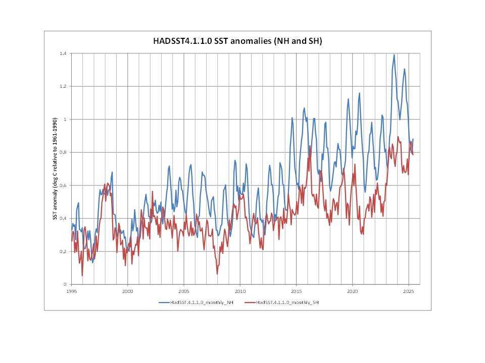
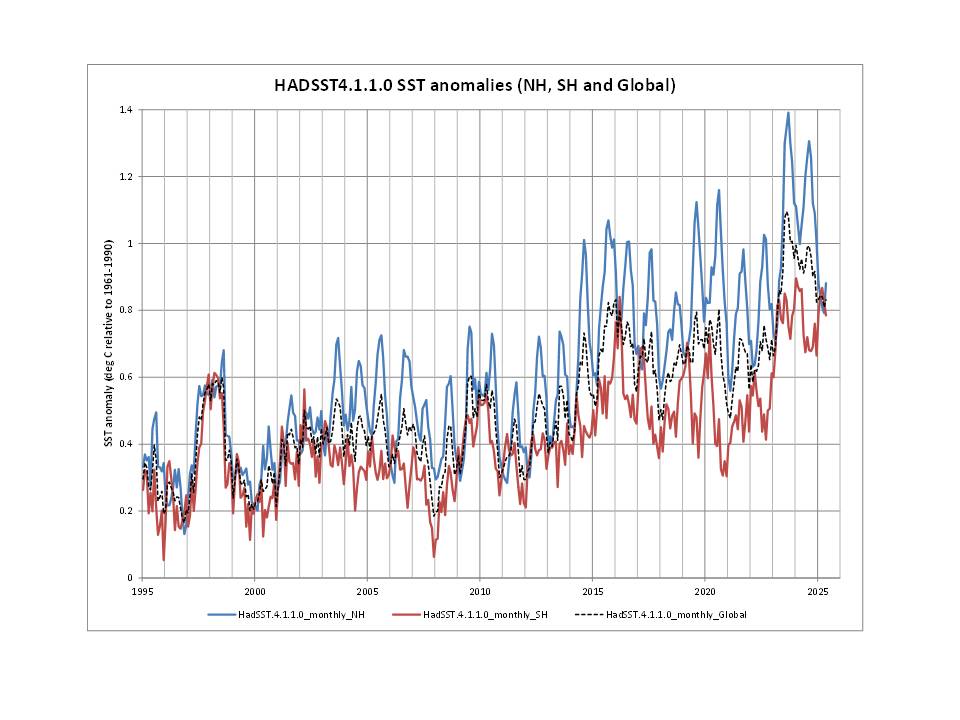
This is an excellent plot … thank you for posting. The timing of the increased coverage around 2005 reminded me of an issue with the northern hemisphere SST data which I highlighted a few years ago. My analysis was based HadSST3 and I shall update to the latest version of HadSST4 as quickly as I can and post it here.
HadCRUT5 is based on a blend of the CRUTEM5 land-surface air temperature dataset and the HadSST4 sea-surface temperature (SST) dataset. In the meantime, here is the earlier HadSST3 data for the northern and southern hemispheres:
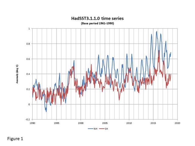
Clearly, the seasonal cycle for the northern hemisphere has not been fully removed after about 2003. Imagine how badly influenced the shape of the temperature profile of the global data would be around the 2015-2016 El Niño. I will leave it at that and get on with preparing graphs based on HadSST4.
New study shows that the summer SST’s in the North Atlantic are colder than basically all the last 10,000 years.
Extended Duration of Abrupt Climate Events From the Early to Late Holocene
Thanks for the link, I need to read that paper.
SE Pacific is also colder than most of the last 2000 years.
Now that I knew. It is in AR6, people forget some regions are cooling, especially in the SH.
Other proxy evidence shows SE Pacific coldest in 10000 years.
Same with the West Pacific warm pool .. pretty much coldest in 10,000 years
As I’ve said before Bnice–you’re smarter than you look.
Thanks for the tip on Rosenthal’s Western Warm Pool papers. The links are:
2018 paper: https://par.nsf.gov/servlets/purl/10224486
and
2017 Paper: https://par.nsf.gov/servlets/purl/10281994
The 2018 paper seems to only be a foreword, but the 2017 one is complete.
Charts starting 1850 with y-axis range detailing 0.1C – what do you do when the data needed to answer an important question does not exist?
Temperatures for all have been recorded as integer values. That immediately means the resolution is ±1.0F. The uncertainty of this resolution is “1/√12 = ±0.3F”. Remember, if a critical uncertainty budget is developed, this value is ADDED to other uncertainties such as repeatability, reproducibility, drift, microclimate changes, and other influence quantities. NOAA shows a ±1.8F (±1.0C) Type B uncertainty for ASOS stations which probably is not far from being correct.
Only if you think CO2 plays a role. The fact is that the solar intensity during the heating season of the NH (March equinox to June solstice) has been trending up since 1700. The solar intensity over the SH during its heating season from September equinox to December solstice has also been increasing but not as much as the NH.
The change in solar intensity during the NH heating season from 1850 to 2025 is up 1.75W/m^2. The change in heating season for the SH over same period is also up but 0.97W/m^2. However these are trends with substantial year to year swings. From 2000 to 2025, the NH heating was up 1.12W/m^2 and the SH heating was up 1.34W/m^2. But the NH has more land and its thermal response to solar forcing is twice as much temperature rise in half the time compared with the SH.
My suggestion for you is to understand the orbital driven solar forcing before condemning the temperature records. I don’t doubt that there are thumbs on the scale of the temperature reporting but there are real changes in orbital driven solar forcing that are going to cause the summer temperature across the NH to increase strongly for millennia before winter snowfall overtakes snow melt and ice is again accumulating.
https://wattsupwiththat.com/2025/05/04/high-resolution-earth-orbital-precession-relative-to-climate-weather/
Those expecting a cooling trend to show up in the NH in coming decades will be disappointed.
The very first question I would ask is, can CO2 and the 15 micron LWIR warm water? It can’t, won’t, and doesn’t. What is warming the oceans is warming the atmosphere, and that is more incoming warming visible radiation is reaching the oceans. The fact that the oceans are warming rules out CO2 as the cause.
https://app.screencast.com/nXfZcUyGR4QlR
Not only that, when you measure the downwelling long wave radiation in the specific CO2 band…
(most hand-helds do not measure in that frequency range. It requires a special type of instrument called a Pyrgeometer.)
… you get a large dip through that CO2 band.
“The very first question I would ask is, can CO2 and the 15 micron LWIR warm water? It can’t, won’t, and doesn’t.”
Of course it can, what is the basis for your assertion?
Of course? Please explain how. 15 micron EMR is strongly absorbed at the surface of the water with minimal penetration. That concentrates the warming to a thin layer. If sufficient energy is absorbed, a molecule of water vapor will be released (latent heat of evaporation) and the heat is removed from the water body. It is a surface phenomena that can’t take place in deep water where it absorbs energy from red and green light.
Why doesn’t Mr May submit his paper to a peer reviewed scientific journal? Or is he not proud of his work?
Yawn! Gets more peer review here than most journals.
Can you counter a single thing he says ?
Because everyone is entitled to maintain some personal standards of association, Wazza.
I was asked to submit a paper presenting the scientific data and reasoning behind the “denier” position. The specific journal (AJES) special issue was supposed to also have papers supporting the alarmist position, and some papers in between. Good idea, I thought! Get it all in the same issue, present both positions, this is really science at its best I thought. The paper is here:
https://onlinelibrary.wiley.com/doi/10.1111/ajes.12579
What followed was a year of Hell. Wiley tried to force the journal to retract our paper, the paper that they invited! The board refused because there was nothing wrong with our paper, no errors were ever found, so Wiley forced them to publish a companion paper criticizing our paper, but there was nothing legitimate to criticize. The editor who asked me to write the paper was fired.
This is why I don’t submit papers to peer reviewed journals, they are totally corrupt and the publishing companies (Wiley and Springer-Nature) are worse.
More on this topic here:
https://andymaypetrophysicist.com/2024/09/27/suppression-of-science-and-inconvenient-truths/
Until the corruption in the peer-reviewed journal world is cleaned up and it becomes scientifically oriented and non-political, I will not be submitting anything to them. They are truly evil.
As evil as the government-subsidized/controlled foghorn of the Corporate Media, used to promote impeachments of Presidents by Schiff-type characters, who asked for and received an autopen-enabled pardon, as did the “select” J6 House Committee, that destroyed inquiry evidence, just in case they needed to save their asses.
Good for you Andy. There is a reason WUWT is a highly regarded and closely monitored by folks who want a scientific approach to what is occurring.
It’s funny how few warmists present papers to Anthony and the editors that have scientific analysis of experimental data of CO2 affecting the dubious global temperature. There are a way too many time series correlations, that use mostly incorrect methods of time series analysis to justify CO2 causing global warming.
Very nice Andy.
Just a thought here. I’m not sure that people really appreciate the massive increase in the number of ships that were in the Pacific during WWII, many of them in areas not considered as part of normal trade routes. Sure, there was a shift in the method of data collection, but I’m unconvinced that the new method was all that much worse than having a bucket of water evaporate away on the deck while the swabbie smoked a cigarette. What’s really striking about WWII in both the N Atlantic and the S Pacific is the striking increase in the density of data, information that we never had before, and likely won’t have again, at least until the cargo cult guys get their wish.
It is your contention that the Warm anomaly around WWII is a data error?
The 1880 Anomaly, WW II warm silhouette and the Current Anomaly we are living could all be caused by the same phenomena.
My contention is the data collected during WWII is poor, see here for more details:
https://andymaypetrophysicist.com/2025/04/17/the-weather-and-climate-of-world-war-ii/
There was huge El Nino during the early part of the war, so it should have been warm then, but I don’t think we know how warm to any degree of accuracy.
Researching I found there were half a million B17 flights alone, over the English Channel during WWII pouring lots of Water Vapor into the Stratosphere. And the Askja 1875 Volcano was a very wet eruption, and of course the HT eruption, in which I think is what this current anomaly we are experiencing is caused by.
And if so, physics indicates that if you put some quantity of water vapor in the Stratosphere it will cause the Globe to warm. Of course, everyone thinks I am off my rocker, but I must stick with the correlation because I have not heard a good reason as to why this cannot be.
Thanks for your reply, and impressive work as always.
B-17s didn’t fly in the stratosphere!
Oh, my goodness, you buy them books, you send them to school, and for what?
Yes, it is, the Stratosphere over the English Channel begins around 30,000 feet.
What is your authority for claiming that B-17s didn’t fly in the stratosphere?
“Near the equator, the lower edge of the stratosphere is as high as 20 km (66,000 ft; 12 mi), at mid-latitudes around 10 km (33,000 ft; 6.2 mi), and at the poles about 7 km (23,000 ft; 4.3 mi)” — Wiki’
B-17 Performance
They did some of the time, but typically a little lower (around 28,000′) according to what I found online.