Guest essay by Joe Born
In a recent post Christopher Monckton identified me as a proponent of the following proposition: The observed decay of bomb-generated atmospheric-carbon-14 concentration does not tell us how fast elevated atmospheric carbon-dioxide levels would subside if we discontinued the elevated emissions that are causing them. He was entirely justified in doing so; I had gone out of my way to bring that argument to his attention.
But I was merely passing along an argument to which a previous WUWT post had alerted me, and the truth is that I’m not at all sure what the answer is. Moreover, semantic issues diverted the ensuing discussion from what Lord Monckton probably intended to elicit. So, at least in my view, we failed to join issue.
In this post I will attempt to remedy that failure by explaining the weakness that afflicts the position attributed (again, understandably) to me. I hasten to add that I don’t profess to have the answer, so be forewarned that no conclusion lies at the end of this post. But I do hope to make clearer where at least this layman thinks the real questions lie.

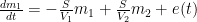
To start off, let’s review the argument I made, which is that the atmospheric-carbon-dioxide turnover time is what determined how long the post-bomb-test excess-carbon-14 level took to decay. That argument was based on the “bathtub” model, which Fig. 1 depicts. The rate at which the quantity <i>m</i> of water the tub contains changes is equal to the difference between the respective rates <i>e</i> (emissions) and <i>u</i> (uptake) at which water enters from a faucet and leaves through a drain:

The same thing can, <i>mutatis mutandis</i>, be said of contaminants (read carbon-14) in the water. But in the case of well-mixed contaminants one of the <i>mutanda</i> is that the rate at which the contaminants leave is dictated by the rate at which water leaves:

where 

Consequently, if the water quantity increases for an interval during which <i>e</i> exceeds <i>u</i>, it will thereafter remain elevated if the emissions rate <i>e</i> then falls no lower than the drain rate <i>u</i>. If a dose of contaminants is added to the water, though, the resultant contaminant amount falls, even when there’s no difference between <i>u</i> and <i>e</i>, in accordance with the <i>turnover</i> rate, i.e., with the ratio of <i>u</i> to <i>m</i>. So, to the extent that this model reflects reality’s relevant aspects, we can conclude that the rate at which the carbon-14 concentration decays tells us nothing about what happens when total-CO2 emissions return to a “normal” level.
But among the foregoing model’s deficiencies is that it says nothing about a possible dependence of overall drain rate <i>u</i> on the water quantity <i>m</i>, whereas we may expect biosphere uptake (and emissions) to respond to the atmosphere’s carbon-dioxide content. Nor does it deal with the possibility that after contamination has flowed out the drain it will be recycled through the faucet. In contrast, the biosphere no doubt returns to the atmosphere at least some of the carbon-14 it has previously taken from it.

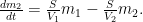
A model that takes such factors into account could support a conclusion different from the one to which the bathtub led us. Consistently with my last post’s approach, Fig. 2 uses interconnected pressure vessels to represent one such model. In this case there are only two vessels, the left one representing the atmosphere and the right one representing carbon sinks such as the ocean and the biosphere.
The vessels contain respective quantities 


Those equations tell us that the carbon quantity 
![m_1(t) = \left[ \frac{V_1}{V_1+V_2}+\frac{V_2}{V_1+V_2} \exp\left(-\frac{V_1+V_2}{V_1V_2}St \right)\right] m_0 ,](https://s0.wp.com/latex.php?latex=m_1%28t%29+%3D+%5Cleft%5B+%5Cfrac%7BV_1%7D%7BV_1%2BV_2%7D%2B%5Cfrac%7BV_2%7D%7BV_1%2BV_2%7D+%5Cexp%5Cleft%28-%5Cfrac%7BV_1%2BV_2%7D%7BV_1V_2%7DSt+%5Cright%29%5Cright%5D+m_0+%2C+&bg=ffffff&fg=000&s=0&c=20201002)
which the substitutions 

Note that in the Fig. 2 system any constituent of the gas would be exchanged between vessels in accordance with the partial-pressure difference of that constituent alone, as if it were the only component the vessels contained. By thus constraining the flow from (and to) the first, atmosphere-representing vessel, this model supports the conclusion that the overall-carbon-dioxide quantity would, contrary to my previous argument, decay just as the excess, bomb-caused quantity of atmospheric carbon-14 did.

Could providing more than one sink enable us to escape that conclusion? Not necessarily. Consider the more-complex system that Fig. 3 depicts. Just as the system that my previous post described, this one can embody the TAR Bern-model parameters. As that post indicated, describing such a system requires a fourth-order linear differential equation. So that system does have more degrees of freedom in its initial conditions and can therefore exhibit a wider range of responses.
But it still constrains the flow among its four vessels linearly in accordance with partial pressures, just as the Fig. 2 system does. From complete equilibrium, therefore, its behavior for any constituent is the same as for any other constituent as well as for the contents as a whole. In other words, this model, too, seems to support the notion that the bomb-test results do indeed tell us how long excess carbon dioxide will remain if we stop taking advantage of fossil fuels.
In a sense, though, the models of Figs. 2 and 3 beg the question; they use the same uptake- and emissions-process-representing
So one question is how significant that difference is in the present context. I don’t have the answer, although my guess is, not very. But readers attempting to answer that question could do worse than start by referring to a previous WUWT post by Ferdinand Engelbeen.

Another way in which carbon-14 differs from the other two carbon isotopes is that it’s unstable. So, if the Fig. 3 model is adequate for carbon-12 or -13, a different model, which Fig. 4 depicts, would have to be used for carbon-14 if its radioactive decay is significant. That diagram differs from Fig. 3 in that it includes a flow 
To the extent that those different models produce different responses, using bomb-test data to predict the total carbon content’s behavior is problematic. But the Engelbeen post mentioned above seems to say that even deep-ocean residence times tend to be only a minor fraction of carbon-14’s half-life: this factor’s impact may be small.
A possibly more-significant factor is that the carbon cycle is undoubtedly non-linear, whereas the conclusions we tentatively drew from the models above depend greatly on their linearity. Before I reach that issue, though, I should point out an aspect of the Bern model that was not relevant to my previous post. The Bern equations I set forth in my last post were indeed linear. But that does not mean that their authors meant to say that the carbon cycle itself is. Although for the sake of simplicity I’ve discussed the models’ physical quantities as though they represented, e.g., the entire mass of carbon in a reservoir, their authors no doubt intended their (linear) models’ quantities to represent only the differences from some base, pre-industrial values. Presumably the purpose was to limit their range enough that the corresponding real-world behavior would approximate linearity.
But such linearization compromises the conclusions to which the models of Figs. 2 and 3 led us. A linear system is distinguished by the fact that its response to a composite stimulus always equals the sum of its individual responses to the stimulus’s various constituents; if the stimulus equals the sum of a step and a sine wave, for example, the system’s response to that stimulus will equal the sum of what its respective responses would have been to separate applications of the step and the sine wave. And this “superposition” property was central to drawing the conclusions we did from those models: the response to a large stimulus is proportionately the same as the response to a small one.

To appreciate this, consider Fig. 5, which depicts scaled values of the Fig. 2 model’s left-vessel total-carbon and carbon-14 contents. Initially, the system is at equilibrium, with zero outside emissions 


At time t = 5, a bolus of carbon-14 appears in the (atmosphere-representing) left vessel. Compared with the total carbon content, the added quantity is tiny, but it is large enough to double the small existing carbon-14 content. As the distance between the red dotted vertical lines shows, the resultant increase in carbon-14 content decays toward its new equilibrium value with a time constant of just about seven years. (I’ve assumed that the processes greatly favor the sink-representing right vessel—i.e., that its “volume” is much greater than the left vessel’s—so that the new equilibrium value is not much greater than the original.)
Now consider what happens at t = 45, when the left vessel’s total-carbon quantity suddenly increases. Although the two quantities are scaled to their respective initial values, this total-carbon increase is orders of magnitude greater than the t = 5 carbon-14 increase. Yet, as the black dotted vertical lines show, the decay of the left vessel’s total-carbon content proceeds just as fast proportionately as the much-smaller carbon-14 content did. As was observed above, this could tempt one to conclude that the carbon-14 decay we’ve observed in the real world tells us how fast the atmosphere would respond to our discontinuing fossil-fuel use.
![clip_image009[1]](http://wattsupwiththat.files.wordpress.com/2013/12/clip_image0091.png?quality=75 "clip_image009[1]")
But now consider what can happen if we relax the linearity assumption. Specifically, let’s say that the Fig. 2 model’s proportionality “constant”

In that plot, the red lines show that the carbon-14 decay occurs just as fast as in the previous plot, the carbon-14 content falling to exp(-1) above its new equilibrium value in around seven years. But the much-larger total-carbon increase brings the system into a lower-efficiency range, so that quantity subsides at a more-leisurely pace, taking over forty years. If such results are any indication, bomb-test results are a poor predictor of how long total-carbon content will settle.
Now permit me a digression in which I attempt to forestall pointless discussion of precisely what the quantities are that the graphs show. I believe the exposition is clearest if it is directed, as in Figs. 5 and 6, to ratios that carbon 14 and total carbon bear to their own initial values. But it appears customary to express the carbon-14 content instead in terms of its ratio to total carbon content. This means that, since total carbon has been increasing, the numbers commonly used in carbon-14 discussions could fall below the pre-bomb values, even though total carbon-14 has in fact increased.
For the sake of those to whom that issue looms large, I have attached Fig. 7 to illustrate how the values for carbon-14 itself could differ from those of its ratio to total carbon in a situation in which new (carbon-14-depleted) carbon is continually injected into the atmosphere.

But that’s a detail. More important is the issue that Fig. 6 raises.
Now, I “cooked” Fig. 6’s numbers to emphasize the point that nonlinearity can undermine conclusions based on linear models. Specifically, Fig. 6 depicts the results of making the flows proportional only to the fifth root of the carbon content.
But non-linearity must have some effect. How much? I don’t know. Together with the differences in behavior between carbon-14 and its stable siblings, though, it is among the considerations to take into account in assessing how informative the bomb-test data are.
As I warned at the top of the post, this post draws no conclusions from these considerations. But maybe the foregoing analysis will prompt knowledgeable readers’ comments that help narrow the issues.
Discover more from Watts Up With That?
Subscribe to get the latest posts sent to your email.
There is still no real evidence of what the CO2 concentration would have been without human emission. For all we know, it could be very near what it is now.
The cartoon drawing of sinks (no sources were included on the drawing) is obviously incorrect. There is an immense amount of CH4 (methane also referred to as ‘natural gas’) that is pushed up through the ocean floor and is pushed up through the continents. If there is immense amounts of CH4 released, the marine biosphere is very effective at using the energy in the CH4 and in precipitating the CO2 out. (William: There are sets of observational data to support the above assertion. I have selected a couple of observational data and anomalies to illustrate the issue. Note the CH4 that is bubbling up from the ocean floor is primordial, very, very low C13 content.) Salby is correct, the majority of the 20th century CO2 increase was not due to anthropogenic CO2 emissions.
The fact that there are specialized bacteria that have developed supports the assertion that there is continual (continual on geological time and continual in terms of the supplying food to a life form) release of CH4 from the ocean floor.
The source of the CH4 is from core of the planet. As the core solidifies, CH4 is extruded. The very, very high pressure of the core provides the force to push the CH4 up through the mantel to eventually reach the surface. There is massive amounts of high CH4 and liquid hydrocarbons beneath the continents (the lighter mass of the CH4 and the liquid hydrocarbons explains why the continents float on the mantel and explains the formation of mountain bands and regions on the continents.)
The following links are connected. The sudden release of CH4 from deep within the earth, causes very, very, large earthquakes, such as the series of earthquakes in Mississippi in New Madrid in the 1800’s. The CH4, methane gas when it is released creates ‘sand boils’. The methane gas release also creates mud volcanoes.
http://news.discovery.com/earth/oceans/bubble-hitchhikers-could-check-greenhouse-gas-131210.htm
Seafloor-dwelling bacteria may hitch a ride on methane bubbles seeping from deep-sea vents, preventing the methane from reaching the atmosphere by eating it up, new research suggests.
The findings, presented here today (Dec. 9) at the annual meeting of the American Geophysical Union, could help explain how such huge amounts of the greenhouse gas methane are belched from the ocean floor, yet somehow never reach the atmosphere.
While much of the methane is locked in an inactive form, at shallower depths, bubbles of methane naturally seep up from mud volcanoes and other cracks in the ocean floor. Yet somehow, very little of this methane reaches the atmosphere.
http://www.bbc.co.uk/news/science-environment-25329813
Dr Susan Hough from the US Geological Survey said: “If you try to make a statistical case there are too few earthquakes in the 19th Century.”
“Seismometers were developed around 1900. As soon as we had them, earthquakes started to look bigger,” explained Dr Hough.
Researchers use historical documents to track down seismic events that occurred before this and assess their magnitude.
Dr Hough believes that many large earthquakes in the 18th and 19th Century have been missed.”
Research suggests that half of all quakes measuring more than 8.5 in magnitude that hit in the 19th Century are missing from records.
William: Looking at the data from a different perspective there has been a significant increase in very large earthquakes in the 20th century. It seems unlikely that historians would have not noticed 8.5 magnitude earthquakes.
As noted the release of CH4 (methane which is also called natural gas) causes very large earthquakes.
http://www.new-madrid.mo.us/index.aspx?nid=132
In the known history of the world, no other earthquakes have lasted so long or produced so much evidence of damage as the New Madrid earthquakes. Three of the earthquakes are on the list of America’s top earthquakes: the first one on December 16, 1811, a magnitude of 8.1 on the Richter scale; the second on January 23, 1812, at 7.8; and the third on February 7, 1812, at as much as 8.8 magnitude.
Sand Boils
The world’s largest sand boil was created by the New Madrid earthquake. It is 1.4 miles long and 136 acres in extent, located in the Bootheel of Missouri, about eight miles west of Hayti, Missouri. Locals call it “The Beach.” Other, much smaller, sand boils are found throughout the area.
Seismic Tar Balls
Small pellets up to golf ball sized tar balls are found in sand boils and fissures. They are petroleum that has been solidified, or “petroliferous nodules.”
Ferdinand Engelbeen says:
December 12, 2013 at 1:38 pm
Lars Magnus Hagelstam says:
December 12, 2013 at 9:43 am
However much CO2 is injected into the athmosphere it will be dissolved in cold raindrops and cold surface water.
Forget raindrops and fresh water: at 0.0004 bar CO2 pressure, the solubility in fresh water is very low. That removes less than 1 ppmv where the raindrops are formed and may increase 1 ppmv where they fall on earth.
Ferdinand, where did you get this from? It is contradicted by fact.. 0.0004 bar CO2 pressure is at 1 atmosphere – this is certainly where all the natural, pure, unpolluted water in the atmosphere is spontaneously joined to any and all carbon dioxide around, forming carbonic acid.
Please, it is simply a fact of physical life that all rain is acidic because it has formed carbonic acid with any and all the atmospheric carbon dioxide around it. Rain is around
5.6-8 pH – each drop from base 7 neutral is ten times greater in acidity.
Carbonic Acid is part and parcel of the Water Cycle, water has a residence time of 8-10 days in the atmosphere.
(Carbon dioxide is also heavier than air, it cannot acculuate in the atmosphere, it will always sink to the surface if no other work is being done on it.)
What you are saying just does not make any sense.
:”Ferd
There is hardly any contact between the ocean surface and the deep oceans (even restricted for biolife): most carbon enters via the sink places and most comes back at the upwelling places.”
An assertion. You keep making the same damn claim and there is no actual data. Instead of analyzing what we actually know, the decay constant of 14CO2, the amount of CO2 released into the atmosphere and the atmospheric [CO2], we have grand sweeping assertions that lead to dead end saturated processes.
What is he point of discussing actual models of kinetic processes, if all you do is state, this is the way it is because this is how water moves. You cannot even separate spacial components when we know the damned order atmosphere, surface, depths.
Ferdinand Engelbeen says:
December 12, 2013 at 2:38 pm
Regarding how long to remove the extra mass.
If the off rate measured for 14C does scale to the whole atmosphere, then equilibrium is roughly maintained by an on rate. A pulse of excess CO2 should be taken up by one or more reservoirs unless there is saturation of these reservoirs or another factor alters the on rate. I suppose we are talking about feedbacks now. But just for fun, let’s say the simple model is correct. What would we expect for an off rate (that is how much CO2 should exit the atmosphere per year)? With 3264 Gton CO2 in atmosphere, a roughly 5 year t1/2 gives us 413 Gton/yr flux. Approximately 450 Gton/yr is estimated from http://www.ipcc.ch/publications_and_data/ar4/syr/en/contents.html and http://en.wikipedia.org/wiki/Carbon_dioxide_in_Earth's_atmosphere.
Not bad for a simple model.
To summarize, there are two conclusions I tentatively come to. 1) Humans cannot be the cause of the rise in CO2 because the rise is much greater than the amount of CO2a that should be present given the simple model and t1/2 of 5 years. 2) There is another natural process at work shifting the equilibrium between CO2 reservoirs such that atmospheric CO2 is rising, that is, the on rate has increased.
Using Oak Ridge Natl. Lab global CO2 emission data (1751-2010), I estimate anthropogenic CO2 is now about 200 Gton of the total CO2 in the atmosphere. If we removed it all, atmospheric CO2 would be about 375 ppmv. This view seems relatively balanced with what we know.
My take: With ocean acidification reducing global ocean surface pH from 8.25 to 8.14, and mentions of ocean hydrogen ion content increasing by 26%, I figure that the upper ocean is in equilibrium with atmospheric CO2 content of 353 PPMV. Recent atmospheric CO2 has been 395 PPMV, 42 PPMV higher. I figure that this means 89.5 metric gigatons of carbon being in the CO2 content of the atmosphere that is in excess of equilibrium with the oceans.
Meanwhile, in the most recent years available, http://www.tyndall.ac.uk/global-carbon-budget-2010 says that the oceans are removing CO2 with about 2.5 gigatons of carbon from the atmosphere. 89.5 divided by 2.5 means “time constant” of above-ocean-equilibrium CO2 is about 35-36 years.
The above carbon budget link also mentions land net sinking (outside anthropogenic land use changes) of CO2 averaging 2 gigatons of carbon per year. This means atmospheric time constant of excess CO2 is 20 years lately. Since one time constant has the oceans and land removing 63% of the above-equilibrium atmospheric CO2, the half-life of atmospheric CO2 calculates to about 14 years. Correction for nonlinearity of increased CO2 increasing hydrogen ions in the oceans probably reduces this 14 year figure slightly.
14 years is not far from Anthony Watts’ “bomb test” results, and considerably less than the 30-95 years mentioned in the Wikipedia article on greenhouse gases.
Hoser,
I’ve done your Excel exercise. What is the basis for your equation:
C = N/K * (1 – e ^ -kt ) + H/(h+k) * (e ^ ht – e ^ -kt ) + (N + H) * e ^ -kt
@ur momisugly Joe Born — Do let us know how your wife is doing. I hope that other driver had collision insurance. Of course it wasn’t your wife’s fault!
Please tell her, “Best wishes from the WUWT folks.”
Janice
P.S. Regardless of whether your assertions or diagrams are completely accurate or not, thank you, so much, for this worthwhile and interesting thread full of excellent comments. ALL YOU SCIENCE GIANTS OF WUWT ARE THE BEST!!
Dr Burns says:
December 12, 2013 at 9:05 pm
Hoser,
I’ve done your Excel exercise. What is the basis for your equation
The equation is a solution of
dC/dt = N + Ho *e^(ht) – kC
C is the concentration of atmospheric CO2
N is the natural level of CO2 flowing into the atmosphere, treated as a constant.
Ho is the initial level of anthropogenic CO2.
k is the previously determined off rate constant for CO2 leaving , t1/2 is about 5 years
h is the rate of CO2a increase, assumed to be exponentially increasing, at least recently.
I already gave the basic strategy for solving problems like this (http://wattsupwiththat.com/2013/11/21/on-co2-residence-times-the-chicken-or-the-egg/#comment-1481426), so we just need to show the homogeneous solution and then solve the rest with boundary conditions.
C = U*V
Homogeneous solution U = A1 * e ^(-kt)
Nonhomogeneous
dV/dt = (N + Ho*e^(ht) ) e^(kt), and not showing every step
V = A2 * [ N/k* (e^(kt) – 1) + Ho/(h+k) * (e ^((h+k)*t) -1 ]
Solutions of C are U*V + U with constants that have to be determined by boundary conditions
Out of convenience, I’m redefining A2, and not writing A1*A2. Both are just constants.
C = A2 * [ N/k* (1 – e^(-kt)) + Ho/(h+k) * (e ^(ht) – e^(-kt)) ] + A1 * e ^(-kt)
At t=0, C = A1 = N + Ho
At t=inf, and h=0, C = A2*(N + Ho)/k = (N + Ho)/k, so A2 = 1.
So
C = N/k * (1 – e ^( -kt) ) + Ho/(h+k) * (e ^( ht) – e ^( -kt) ) + (N + Ho) * e ^( -kt)
Because we are using XL, we need to correct for yearly iteration error.
Model steady-state
-0.13540755 1/k = 7.385112595 The expected steady-state level with const 1/y input
year f CO2 corr = 0.935260769 Use this value instead of 1.
0 1
1 1.80862067 <-[=B5*EXP(A$3)+$D$4]
2 2.514837539
3 3.131619035
4 3.670291261
5 4.140745983
6 4.551622273
7 4.91046515
8 5.223864129
9 5.49757423
10 5.736621658
11 5.945396096
12 6.127731318
13 6.28697559
14 6.426053152
15 6.547517917
16 6.653600373
17 6.746248536
18 6.827163727
19 6.897831809
20 6.959550479
21 7.013453091
22 7.06052947
23 7.101644093
24 7.137551955
25 7.168912442
…
83 7.385102702
84 7.385113339
This should help you understand what I did.
Ew. That got a little ugly.
k is 0.13540755 In the sample equation,
B5 is the value in the cell above (i.e. 1) .
We want to decay that amount by 1 year using the exponential term.
Finally, we would have added 1 each year, but because we are iterating only once per year, we pre-decay that value adding the value 0.935260769 instead. It comes in as $D$4 in the sample equation.
Count_to_10 says:
December 12, 2013 at 4:38 pm
There is still no real evidence of what the CO2 concentration would have been without human emission. For all we know, it could be very near what it is now.
From the 800 kyr past, measured in ice cores, we know that there was a quite strict equilibrium between CO2 and temperature of around 8 ppmv/°C. The evidence from the past is that for the current temperature the equilibrium CO2 level would be around 290 ppmv. Currently we are some 110 ppmv above that equilibrium:
http://www.ferdinand-engelbeen.be/klimaat/klim_img/antarctic_cores_001kyr_large.jpg
“There are exchanges by bio-life, but as bio-life in the oceans is not CO2 starved contrary to land plants, more CO2 in the oceans has no influence on bio-life.”
An interesting assertion. Is it verified?
Myrrh says:
December 12, 2013 at 5:20 pm
Ferdinand, where did you get this from? It is contradicted by fact.. 0.0004 bar CO2 pressure is at 1 atmosphere – this is certainly where all the natural, pure, unpolluted water in the atmosphere is spontaneously joined to any and all carbon dioxide around, forming carbonic acid.
Most CO2 in circulation comes from the warm oceans, where water vapour and CO2 are lifted off from the surface up to the formation of clouds and rain. The solubility of CO2 in water at 1 bar (pure CO2!) is 3.3 g/l at 0°C, see:
http://www.engineeringtoolbox.com/gases-solubility-water-d_1148.html
The solubility of any gas in a liquid is directly in ratio to its partial pressure, no matter if that is in full vacuum or surrounded with 99.9996% of other molecules. Thus the solubility of CO2 at its own partial pressure is 3.3 g * 0.0004 bar = 1.32 mg/l. That indeed gives the low pH of (clean: no SO2 or NOx) rain.
At the cloud side, you need 400 m3 of air to condense 1 liter of water (if I remember well from some previous calculation). Taking 1.32 mg CO2 out of 400 m3 of air is unmeasurable.
At the ground side, if all CO2 would come out of 1 mm rain (1 l/m2), that increases the CO2 level of the adjacent 1 m3 of air with less than 1 ppmv, assuming there is no wind to mix the air masses.
Thus while the total carbon mass circulating via clouds/rain still is huge, thanks to the huge water masses, it hardly influences local CO2 levels and as most of the water cycle is very short, it doesn’t influence global CO2 levels.
Carbon dioxide is also heavier than air, it cannot acculuate in the atmosphere, it will always sink to the surface if no other work is being done on it.
There is sufficient work done by wind and molecular movements to keep CO2 in the atmosphere, where similar levels (+/-2% of full scale) are found up to 20 km height. Only in stagnant air as can be found in accumulating snow (firn), there is a 1% increase of CO2 at the bottom of the firn after 40 years, for which is compensated in the calculations. Not a big problem…
David A says:
December 13, 2013 at 1:26 am
An interesting assertion. Is it verified?
Have a look at the total dissolved inorganic carbon (DIC – CO2+bicarbonate+carbonate) in seawater over the seasons, you can see that biolife increases in summer (more sunlight, higher temperatures). The difference is 30 μmol/kg over 2030-2060 μmol/kg or a difference of 1.4% of total inorganic carbon. Even if biolife increased a tenfold, there still would be abundant carbon available:
http://www.biogeosciences.net/9/2509/2012/bg-9-2509-2012.pdf (Fig. 4).
The main restriction of life in seawater is a lack of minerals and nutritients, reason why there is abundant sealife at upwelling places, bringing minerals, N and P to the surface…
Ferdinand Engelbeen says:
December 12, 2013 at 1:58 am
phlogiston says:
December 12, 2013 at 12:53 am
A radiotracer measures a single removal term. PERIOD. A pulse of CO2 enters the atmosphere different from the other CO2 due to 14C. So it can be tracked in exclusion of any other CO2.
In this case, the radiotracer meausures not only the removal term (as mass), but also the “thinning” of the concentration, because what returns from the deep is only halve the concentration (at the height of the bomb spike) of what goes into the deep oceans. Two distinct removal rates without much connection with each other.
The decay rate of a 12CO2 pulse only depends of the mass balance between ins and outs, the decay rate of a 14CO2 pulse mainly depends of the concentration balance and hardly the (total) mass balance between ins and outs.
Your 7 lines of reply are still much too complicated. And the mention of “deep ocean” indicates that, WADR, you still don’t get it.
The only real question as to the validity of the bomb 14CO2 loss data is that of the extent and speed of atmospheric mixing at the start. I’m not clear if you were referring to this. But this probably has the potential to modify the 5 year result only a minor way.
Everyone here who talks about recycling shows that they don’t understand the first thing about a kinetic measurement.
It is an essential prerequisite of an effective kinetic tracer that it is NOT recycled back into the measured compartment. So the fact that bomb 14CO2 is not returned from sea to atmosphere serves only to underpin the validity of this measurement of 5 year t1/2 removal of CO2 from the atmosphere.
Lars Magnus Hagelstam says:
December 12, 2013 at 9:43 am
The relevant issue is water.
98% of the CO2 in the lithosphere is dissolved in water as COC03.
The part pressure of gazeous CO2 in the athmosphe is a function of the proportion of CO2 in the water and its temperature (Henry’s law). Think cold beer, warm beer.
However much CO2 is injected into the athmosphere it will be dissolved in cold raindrops and cold surface water.
And that is why the whole of the Water Cycle has been expunged from AGW influenced education – even at university level – and so precipitation taken out of the Carbon Cycle and out of the models.
Here is an example of the zilch mention of our great water cycle with its turnover of 8-10 days in the atmosphere which clears away all the carbon dioxide around it – solely to avoid jarring with the “meme” that “CO2 accumulates for hundreds and thousands of years in the atmosphere” :
http://www.columbia.edu/~vjd1/carbon.htm
How can there possibly be any educated description of the Carbon Cycle which eliminates precipitation? Only in the AGW faked physics being inculcated into the education system. The enormity of this brainwashing is not apparent to most, because they have been brainwashed..
The AGW claims begin by corrupting basic physics and are perpetuated by arguments, as from Ferdinand, by those who not know the real basics.
It is impossible to see that the Water Cycle has been excluded from the AGW version of the Carbon Cycle unless one knows the real basics that water in the atmosphere form carbonic acid with any and all carbon dioxide around, in rain, fog, dew..
As the Columbia page shows, AGW only admits to water forming carbonic acid with carbon dioxide at the ocean level, missing out the exact same physical processess in the atmosphere.
They have substituted “sinks” for the natural dynamic cycles which continually clear away carbon dioxide; which cannot accumulate in the atmosphere anyway because it is heavier than air. And this too has been written out of the AGW “climate physics”, but this time not by simply expunging all mention of it, but by changing the physical properties of carbon dioxide, by the simple but effective fib that it is an “ideal gas” without properties, therefore, for example, without attraction, weight relative to air etc.
This is a clever and well thought out manipulation of the basic physical properties of matter which have now become accepted ‘science facts’ by the majority. I would like to have been able to say ‘non-specialists’, but these manipulated facts have become so ingrained through education that even those who should know, climate scientists, do not.
What we have is a whole generation of climate scientists who do not question the AGW claims of the ability of carbon dioxide to accumulate in the atmosphere because they have not been taught the real physical properties of gases, but faked. The dog that didn’t bark.
That is the primary reason these discussions become so convoluted..
Ferdinand Engelbeen: ,
,  , and
, and  at which it flows into the general mixed layer, the uptake (downwelling) region, and the emissions (upwelling) regions. For the sake of simplicity, we’ll consider those three quantities not actually as flow rates but rather as components of partial-pressure change rate. To determine the partial-pressure-change components caused by flow the other way, i.e., into the atmosphere, we’re going to assume that the partial pressure in the emissions region is some fixed fraction
  of the general mixed-layer partial pressure
  and that the partial pressure in the emissions region is some multiple
  of what we’re going to assume for the sake of simplicity is a fixed historic pressure
  . So that component will be a quantity
  proportional to external emissions (including, in deference to Dr. Brown, CO2 from volcanoes) plus quantities
  ,
,  , and
, and  proportional to flows from the mixed layer, uptake region, and emissions regions. That is,

 :
:

 and the addition of a cosmic-ray-related rate
  :
:


As I warned, I haven’t run out of questions.
Here’s how I’ve translated for myself what you’ve told me. Here I’m going to forget about the biosphere and not explicitly keep track of the deep oceans. (No, wait, hear me out; I think it makes sense.)
The rate of CO2 flow from the atmosphere is proportional to the sum of the respective rates
We’ll also assume that the mixed layer turns over (through the deep layer) at a rate
For 14CO2, it appears that the equations are exactly the same except for a beta-decay factor
How am I doing so far?
“Joe Born
to
Ferdinand Engelbeen:
The rate of CO2 flow from the atmosphere is proportional to the sum of the respective rates k_{am}P_a, k_{au}P_a, and k_{ae}P_a at which it flows into the general mixed layer, the uptake (downwelling) region, and the emissions (upwelling) regions.”
Just wait a moment Joe and think about what Ferdinands 5% upwelling means.
The surface of the ocean holds about 870 GtC, and the concentration of dissolved inorganic carbon is about 1.9 mM.
The depths have a dissolved inorganic carbon concentration of about 2.3 mM; if Ferdinand is correct about the 5% figure, then annually, 5% of the surface (1.9mM) goes down and is replaced by deep water (2.3mM DIC), giving an overall trafficking to the surface of 7 GtC per year.
This is not a problem as long as the rate of carbon transport at the surface is greater than 7 GtC.
As stated previously, the surface layer is denuded of inorganic carbon as photosynthesis converts it to organic matter, a large fraction of which sinks to the depths, where it is recycled into DIC by anaerobic and aerobic microorganisms.
Focusing on a single rate or mechanism makes a mockery of the whole point of simplistic box modeling. Box modeling is a way to look as fluxes throughout the whole system, allowing you to identify where to look for a mechanism.
phlogiston says:
December 13, 2013 at 2:28 am
Everyone here who talks about recycling shows that they don’t understand the first thing about a kinetic measurement.
So the fact that bomb 14CO2 is not returned from sea to atmosphere serves only to underpin the validity of this measurement of 5 year t1/2 removal of CO2 from the atmosphere.
————————————————
Amen to that too.
I think the resistance to assimilating the actual, real data, such resistance manifesting itself as pages and pages of mental masturbation, is because plugging in that real number for the half-life (probably the most important number of all) destroys the mass balance argument and many other such preconceived conclusion-based arguments.
Strange, because it’s not a big secret that most preconceived conclusion-based arguments end up in the flushed toilet of science history.
This is chemical kinetics 101. The radiotracer “experiment” is giving a kinetic rate constant of a one way reaction in an albeit complex and reversible reaction. Use it.
kwinterkorn: “It bothers me that the biosphere absorptions and emissions of CO2 as a function of both pCO2 in the atmosphere and seas, and in response to global temperatures, are not included quantitatively in the discussion.”
Your various observations that followed the above excerpt have merit, of course. What I presented were just toy models–if that term isn’t redundant–used to think about a highly circumscribed issue, namely, how much bomb-test results tell us about the tenacity of the overall CO2 level. That said, Vessel 2 in Fig. 3 could be considered to reflect the effects of pCO2 (but not temperature) on the biosphere.
Incidentally, I may not remember this correctly, but I believe Mr. Engelbeen is of the opinion that biology has only a negligible effect on the oceans’ CO2 behavior.
Ferdinand Engelbeen: “Hope that you don’t have too much damage at your (wife’s ?) car”
Janice Moore: “Do let us know how your wife is doing”
Thank you for asking. Physically she’s fine. And a nice glass of wine fixed her up emotionally as well. I don’t have a damage estimate yet.
(As to whose fault, the less said the better.)
Janice Moore: “ALL YOU SCIENCE GIANTS OF WUWT ARE THE BEST!!”
I think they are, too, although, understandably, we have to pick and choose. I find doing that difficult, but it’s an unfortunate fact that current events make blundering through this stuff necessary if we’re to be informed citizens.
DocMartyn: “The surface of the ocean holds about 870 GtC, and the concentration of dissolved inorganic carbon is about 1.9 mM.
“The depths have a dissolved inorganic carbon concentration of about 2.3 mM; if Ferdinand is correct about the 5% figure, then annually, 5% of the surface (1.9mM) goes down and is replaced by deep water (2.3mM DIC), giving an overall trafficking to the surface of 7 GtC per year.
This is not a problem as long as the rate of carbon transport at the surface is greater than 7 GtC.”
Can you help me out here? I hope I haven’t misrepresented myself, but I’m just a layman doing the sums, so the implications of your statements, while no doubt obvious to most of this site’s denizens, are a bit of a reach for me.
First off, I didn’t see where the “7 GtC” came from. I would have inferred from your other numbers that the “overall tracking to the surface” would be 870 GtC * (2.3 mM – 1.9 mM) / (1.9 mM) = 9.2 GtC.
Second, although you quoted my first equation’s quantities that with flows from the atmosphere to the oceans, I would have thought your observations were more relevant its remaining quantities, which, deal with flows from the oceans to the atmosphere. As to those, my (no doubt forlorn) hope would be that the h_u and h_e fudge factors, together with the fact that the k’s may make at least some stab at taking not only the dissociation but also the biological loss into account, might enable me nonetheless to make some sense of what Mr. Engelbeen has explained to me.
Again, remember that I’m no scientist, so I’ll be grateful if you can indulge me by being less elliptical.
Rounding without coffee and calculator.
Down-welling of 5% of 870 GtC, 43.5 GtC, at about 19.5 mM DIC.
The same volume is replaced by deep ocean water with 23 mM DIC, so total carbon =(23/19.5)*43.5 GtC, 51.3 GtC. Delta is about 7.8.
The range is about 7-9 GtC.
The problem we have with polar waters as down welling ‘sinks’ for DIC, based on Henry’s law, is that these polar oceans at the edge of the ice caps are highly bio-productive and the surface is denuded of DIC during the summer months.